Longitudinal Data Analysis Using Multilevel Linear Modeling (MLM): Fitting an Optimal Variance-Covariance Structure

(1)

LONGITUDINAL DATA ANALYSIS USING MULTILEVEL LINEAR MODELING (MLM): FITTING AN OPTIMAL VARIANCE-COVARIANCE

STRUCTURE

A Dissertation by

YUAN-HSUAN LEE

Submitted to the Office of Graduate Studies of Texas A&M University

in partial fulfillment of the requirements for the degree of DOCTOR OF PHILOSOPHY

August 2010

(2)

Longitudinal Data Analysis Using Multilevel Linear Modeling (MLM): Fitting an Optimal Variance-Covariance Structure

(3)

LONGITUDINAL DATA ANALYSIS USING MULTILEVEL LINEAR MODELING (MLM): FITTING AN OPTIMAL VARIANCE-COVARIANCE

STRUCTURE

A Dissertation by

YUAN-HSUAN LEE

Submitted to the Office of Graduate Studies of Texas A&M University

in partial fulfillment of the requirements for the degree of DOCTOR OF PHILOSOPHY

Approved by:

Co-Chairs of Committee, Victor L. Willson Oi-Man Kwok Committee Members, Robert Hall

F. Michael Speed Head of Department, Victor L. Willson

August 2010

(4)

ABSTRACT

Longitudinal Data Analysis Using Multilevel Linear Modeling (MLM): Fitting an Optimal Variance-Covariance Structure. (August 2010)

Yuan-Hsuan Lee, B.A., National Tsing Hua University Co-Chairs of Advisory Committee: Dr. Victor L. Willson

Dr. Oi-Man Kwok

This dissertation focuses on issues related to fitting an optimal variance-covariance structure in multilevel linear modeling framework with two Monte Carlo simulation studies.

In the first study, the author evaluated the performance of common fit statistics such as Likelihood Ratio Test (LRT), Akaike Information Criterion (AIC), and Bayesian Information Criterion (BIC) and a new proposed method, standardized root mean square residual (SRMR), for selecting the correct within-subject covariance structure. Results from the simulated data suggested SRMR had the best performance in selecting the optimal covariance structure. A pharmaceutical example was also used to evaluate the performance of these fit statistics empirically. The LRT failed to decide which is a better model because LRT can only be used for nested models. SRMR, on the other hand, had congruent result as AIC and BIC and chose ARMA(1,1) as the optimal

variance-covariance structure.

In the second study, the author adopted a first-order autoregressive structure as the true within-subject V-C structure with variability in the intercept and slope

(5)

iv

(estimating and only) and investigated the consequence of misspecifying different levels/types of the V-C matrices simultaneously on the estimation and test of significance for the growth/fixed-effect and random-effect parameters, considering the size of the autoregressive parameter, magnitude of the fixed effect parameters, number of cases, and number of waves. The result of the simulation study showed that the commonly-used identity within-subject structure with unstructured between-subject matrix performed equally well as the true model in the evaluation of the criterion variables. On the other hand, other misspecified conditions, such as Under G & Over R conditions and Generally misspecified G & R conditions had biased standard error estimates for the fixed effect and lead to inflated Type I error rate or lowered statistical power.

The two studies bridged the gap between the theory and practical application in the current literature. More research can be done to test the effectiveness of proposed SRMR in searching for the optimal V-C structure under different conditions and evaluate the impact of different types/levels of misspecification with various specifications of the within- and between- level V-C structures simultaneously.

(6)

DEDICATION

This dissertation is dedicated to Michelle and Katherine, my two beautiful and precious gifts from God.

(7)

vi

ACKNOWLEDGEMENTS

I am proud of being a member of Research, Measurement, and Statistic Program at Texas A&M University. The training in the program equipped me with the

professional knowledge of a quantitative methodologist. Particularly, I am grateful for my co-chairs, Dr. Oi-Man Kwok and Dr. Victor Willson, for their guidance through my doctoral study. Dr. Kwok is a wonderful adviser, who leads me to the world of

quantitative and statistical research step by step and is always willing to share his experiences in academia. Dr. Willson has my deepest respect. I admire his insight and passion in quantitative research. More often than not, I am surprised by his brilliant and enlightening comments in research. He always reminds me of linking the simulations to real situations. I am also thankful for my committee members, Dr. Robert Hall and Dr. Mike Speed. They are very supportive in my doctoral study. I learned advanced mixed effects modeling from Dr. Speed, who helped me a lot in the data generation of study two. I also would like to thank Dr. Bruce Thompson and Dr. Myeongsun Yoon. The beginning statiscs courses I took from Dr. Thompson are sure to have a great impact on me for a life time. The measurement and IRT knowledge I learned from Dr. Yoon patched my knowledge in RMS. Of all the professionals, I also like to thank Dr. Hersh Waxman. It is my greatest honor to work for Dr. Waxman. Under his supervision, I learned how to work on research and complete a project as a team. He gave me great flexibility and opportunities to apply what I have learned in real research. Most

(8)

important of all, I am impressed that he is such a great scholar who shows respect to his colleagues and is surprisingly humble.

I would like to thank my parents who brought me up and strived to provide me with a good education. I was pregnant with my second child when working on my dissertation. Without their help with the baby and everyday chores, I would never have finished my dissertation and passed my final defense successfully. Thank you, dad and mom! I love you!

Finally, I need to thank Jerry Jiun-Yu Wu, my dear husband. He is the one who makes me so productive such that I have two beautiful daughters and an earned

(9)

viii TABLE OF CONTENTS Page ABSTRACT ... iii DEDICATION ... v ACKNOWLEDGEMENTS ... vi

TABLE OF CONTENTS ... viii

LIST OF TABLES ... xi

LIST OF FIGURES ... xii

1. INTRODUCTION ... 1

1.1 Organization of Dissertation ... 3

2. REVIEW OF ISSUES RELATED TO MULTILEVEL LINEAR MODELING ... 5

2.1 Advantages of MLM ... 6

2.1.1 Unbalanced Data or Missing Data Points ... 6

2.1.2 No Requirement for Observations to Be Taken Equidistantly ... 6

2.1.3 Capturing the Average Growth Trend over Time ... 6

2.1.4 Flexibility in Modeling the V-C Structure ... 7

2.2 MLM as Mixed Effect Models ... 8

2.3 Estimation Method ... 10

2.3.1 Fixed Effect ... 11

2.3.2 Random Effect ... 12

2.4 Types of Variance-Covariance Structures ... 13

2.4.1 Identity Structure (ID) ... 15

2.4.2 Compound Symmetric (CS) ... 15

2.4.3 First-Order Autoregressive (AR(1)) ... 15

2.4.4 First-Order Autoregressive Moving Average Model (ARMA(1,1)) ... 16

2.4.5 Toeplitz (TOEP) ... 16

2.4.6 Unstructured (UN) ... 16

2.5 Effect of Misspecifying the Within-Subject V-C Structure and Types of Misspecification ... 17

2.6 Selecting an Optimal V-C Structure ... 18

(10)

Page

2.6.2 Akaike Information Criteria (AIC) ... 20

2.6.3 Bayesian Information Criteria (BIC) ... 21

2.6.4 Standardized Root Mean Square Residual (SRMR) ... 22

2.7 Discussion ... 23

3. SEARCHING FOR THE OPTIMAL WITHIN-SUBJECT COVARIANCE STRUCTURE IN LONGITUDINAL DATA ANALYSIS USING MULTILEVEL MODELING (MLM): A MONTE CARLO STUDY ... 25

3.1 Theoretical Framework ... 25

3.2 Method ... 26

3.2.1 Research Design and Model Parameterization ... 27

3.2.2 Selection Criterion for the Optimal Covariance Matrix ... 29

3.3 Result ... 31

3.3.1 Convergence Rate ... 31

3.3.2 AIC and BIC Hit Rate ... 31

3.3.3 SRMR Hit Rate ... 35

3.3.4 Likelihood Ratio Test ... 38

3.4 Demonstration with Empirical Data ... 41

3.4.1 Result for Empirical Data ... 41

4. EVALUATING THE IMPACT OF DIFFERENT TYPES/LEVEL OF MISSPECIFICATION IN THE WITHIN- AND BETWEEN-SUBJECT VARIANCE-COVARIANCE MATRICES IN MULTILEVEL MODELS WITH LONGITUDINAL DATA ... 45

4.1 Theoretical Framework ... 45

4.2 Purpose of This Study ... 46

4.3 Method ... 47

4.3.1 Model Specification ... 48

4.3.2 Evaluation Criterion ... 52

4.4 Result ... 53

4.4.1 Convergence of Analysis ... 53

4.4.2 Relative Bias and Simple Bias for the Fixed Effect ... 54

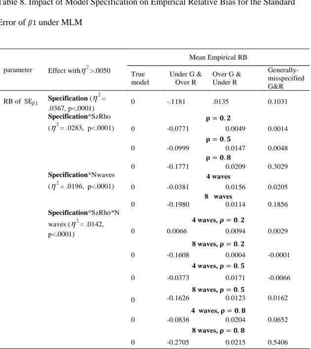
4.4.3 Empirical Relative Bias for the Standard Error of the Fixed Effect ... 54

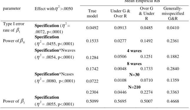
4.4.4 Type I Error Rate of Detecting and ... 59

4.4.5 Statistical Power of Detecting and ... 60

(11)

x

Page REFERENCES ... 67 APPENDIX A ... 74 VITA ... 82

(12)

LIST OF TABLES

Page

Table 1. AIC Hit Rate ... 33

Table 2. BIC Hit Rate ... 34

Table 3. Four-Way Analysis of Variance for AIC and BIC Hit Rate ... 36

Table 4. SRMR Hit Rate ... 37

Table 5. Four-Way Analysis of Variance for SRMR Hit Rate ... 39

Table 6. LRT Hit Rate ... 40

Table 7. Values of Fit Statistics on Four Imposed Σ with Empirical Data. ... 42

Table 8. Impact of Model Specification on Empirical Relative Bias for the Standard Error of under MLM ... 56

Table 9. Impact of Model Specification on Empirical Relative Bias for the Standard Error of under MLM ... 58

Table 10. Impact of Model Specification on the Significance Test for Linear Growth Model under MLM ... 61

(13)

xii

LIST OF FIGURES

Page Figure 1. Commonly Used Within-Subject V-C Structure. ... 14 Figure 2. Illustration of True Between- and Within-Subject Variance-Covariance

Structure and 3 Misspecified Conditions in the Between- and

(14)

1. INTRODUCTION

Quantitative researchers have made extensive use of multilevel linear modeling (MLM) technique to analyze repeated measurement data. MLM has several advantages over traditional methods Univariate Analysis of Variance (UANOVA) or Multivariate Analysis of Variance (MANOVA) in analyzing repeated measures or longitudinal studies, such as allowing unbalanced data or missing data points, not requiring observations taken equidistantly, capturing the average growth trend of the outcome variable over time, and flexibly modeling the variance-covariance (V-C) structure (Diggle, 1988; Ferron, Dailey, & Yi, 2002; Laird & Ware, 1982; Luke, 2004; Wolfinger, 1993). The focus of this dissertation focuses on the last advantage, that V-C structure in MLM can be flexibly specified. Though MLM allow flexibly modeling of the V-C structure, the default V-C matrix in most of the commonly used statistical packages is still the identity structure, which assumes equal variance of each observation and no covariance between any pair of repeated measures. Careless or inexperienced researchers in performing MLM studies may just leave the choice of V-C structure to the computer software. Misspecification in the covariance structure in MLM or leaving the

specification of V-C structure to the computer software generally causes no harm to the estimation of fixed effect /growth parameters (Ferron et al., 2002; Kwok, West, & Green, 2007; Murphy & Pituch, 2009); however, the corresponding estimates for the ____________

(15)

2

standard errors of the fixed effect/ growth parameters are biased, which will in turn lead to erroneous statistical inference of the hypothesis testing results (Davis, 2002; Diggle, Heagerty, Liang & Zeger, 2002; Kwok et al., 2007; Singer & Willett, 2003).

To motivate the use of MLM methodology, the second section of this dissertation reviews issues related to MLM: its advantages over traditional methods, MLM as a mixed effect model, effects of misspecifying the within-subject V-C Structure, types of misspecification, and existing methods in selecting an optimal V-C structure. Through the review of MLM, two research issues emerge and draw our attention. First, there is a lack of an optimal model selection method, and second, the effect of different

types/levels of misspecification has not been investigated. As mentioned previously, misspecification of the within-subject V-C structure, although it may not have a negative influence on the fixed effect estimates, leads to biased estimation in the standard errors for the fixed effect. In other words, the statistical inferences drawn from the combination of unbiased fixed estimates and biased standard errors of the fixed effects will still be erroneous. This issue requires development of effective methods in selecting an optimal within-subject V-C structure, which is the third section of the dissertation. In section 3, the performance of LRT, AIC, BIC, and SRMR on searching for the correct covariance structure will be evaluated. The impact of several design factors, such as number of cases, number of repeated measurements, magnitude of the average growth model, and magnitude of the between-subject covariance matrix on the performance of these search methods, are also considered in the analysis.

(16)

A second consideration is that misspecification in both the between-subject (G -side) and the within-subject (R-side) covariance structure has rarely been examined simultaneously compared to misspecification of the within-subject V-C structure, which has been researched extensively (Ferron et al., 2002; Kwok et al., 2007; Murphy & Pituch, 2009; Vallejo, Ato, & Valdés, 2008). In a simple linear growth curve model, the G matrix is comprised of random effects, including variance of intercept ( ), variance of slope , and covariance between intercept and slope ( ), capturing the deviation of growth parameters from the population means for intercept and slope. Therefore, when fitting a mixed effect model for repeated measurements, researchers need to specify both the G- and R- side V-C structure for the data. In the best scenario, researchers will specify the V-C structures for the two sides correctly. In other cases, researchers may over-, under-, or generally misspecify the V-C structures. The fourth section of the dissertation will investigate the effects of different types and levels of misspecification in both the G and R side on the estimation of growth parameters, their corresponding standard errors, Type I error rate of the fixed effects, and the empirical statistical power for nonnull conditions.

1.1 Organization of Dissertation

The present dissertation is divided into five distinct sections. Sections 3 and 4 are written as individual manuscripts for potential publication in peer-reviewed journals. How each of the sections is conceptualized is presented below:

Section 1 serves as an introductory section that provides a brief overview of the topics to be examined along with a theoretical rationale for each of the individual

(17)

4

studies. Section 2 provides a comprehensive literature review of issues related to MLM, including its advantages over traditional methods, MLM as a mixed effects model, the effects of misspecifying the within-subject V-C Structure and types of misspecification, and a review of existing methods in selecting an optimal V-C structure. Section 3 reports a Monte Carlo simulation study investigating the performance of commonly used fit statistics (i.e., AIC, BIC, Likelihood Ratio Test) in selecting the optimal V-C structure. A new index, Standardized Root Mean Square Residual (SRMR), is also proposed and evaluated. Annotated syntax is given to show how SRMR is calculated using Matlab. The third section is the first journal article. Section 4 reports results of a Monte Carlo simulation study that examines the effect of different types/levels of V-C

misspecification in both the between- and within-subject matrices. The fourth section is the second journal article. Section 5, the last section, is the concluding section that connects the findings from the three manuscripts to provide overall and specific remarks for conclusions about MLM.

(18)

2. REVIEW OF ISSUES RELATED TO MULTILEVEL LINEAR MODELING

Multilevel linear modeling (MLM) for repeated measurement data has drawn increased attention in social and psychological studies over the past few decades. MLM is widely used for longitudinal studies because, for example, it can track the change of normal growth, identify risk factors, and assess the effect of intervention (Raudenbush, 2001). There are several advantages of modeling repeated measurement data using MLM over conventional statistical methods, such as (1) allowing unbalanced data or missing data points, (2) no requirement for observations to be taken equidistantly, (3) capturing the average growth trend of the outcome variable over time, and (4) flexibly modeling the variance-covariance (V-C) structure. Though MLM has many advantages over traditional methods, several issues remain unsolved and there are pitfalls that researchers may accidentally fall into when they do not have a thorough understanding of the MLM methodology. This section reviews the common issues related to MLM and is intended to function as a guide to introduce novice MLM researchers in the use of MLM to analyze repeated measurement data. It includes the advantages of MLM, MLM as a mixed effect model, effect of misspecifying a within-subject V-C structure, and methods in selecting an optimal V-C structure.

(19)

6

2.1 Advantages of MLM 2.1.1 Unbalanced Data or Missing Data Points

MLM does not require data to be balanced, where there are equal numbers of observations for all the combination of the classification factors, and allows analysis with missing data (Luke, 2004). Traditional Multivariate Analysis of Variance

(MANOVA) deletes all the individuals or experimental units with missing data points (Hedeker & Gibbons, 2006); on the contrary, MLM uses all the available data, and the requirement of complete data is not necessary in the MLM analysis because the estimation method in MLM software packages such as PROC MIXED in SAS uses likelihood-based ignorable analysis, which assumes data to be missing at random (MAR), which can lead to valid analysis (Verbeke & Molenberghs, 2000).

2.1.2 No Requirement for Observations to Be Taken Equidistantly

Even if researchers can overcome the first constraints in traditional analysis methods and have complete data, equally-spaced observations will be required for both MANOVA and repeated measure ANOVA (Hedeker & Gibbons, 2006). In MLM, observations need not to be taken equidistantly. MLM can model pattern of change at unequally spaced time points as well as fixed time points.

2.1.3 Capturing the Average Growth Trend over Time

MLM allows the modeling of initial status and growth curve of each individual on an outcome variable. MLM has the capacity to depict the individual growth trend and the variation in the growth curve. The modeling of change is usually conducted in two

(20)

levels, with level one being a function of time and level two examining individual difference in growth rate and initial status (Ferron et al., 2002). Repeated measure ANOVA, however, treat repeated measures as a within-subject factor on a nominal scale and can only test the difference in the response variable means at the different time points; similarly, the focus of MANOVA is on group mean comparison and gives no person-specific growth curves (Hedeker & Gibbons, 2006).

2.1.4 Flexibility in Modeling the V-C Structure

Most importantly, the focus of this paper is related to the advantage that the variance-covariance (V-C) structure can be flexibly modeled in MLM (Diggle, 1988; Laird & Ware, 1982; Wolfinger, 1993) while conserving degrees of freedom compared to unstructured modeling. Traditional UANOVA for repeated measurements requires the sphericity assumption or Huynh-Feldt (H-F) condition (with a compound symmetry V-C structure as the sufficient condition) which implies equal error variance for each measure within an individual and constant correlation between any pairs of repeated measures. This compound symmetry V-C structure may not be suitable for longitudinal data given that measures within a subject tend to correlate over time and the association diminishes as lags in time decreases (Hedeker & Gibbons, 2006). On the other hand, Multivariate Analysis of Variance (MANOVA) assumes an unconditional V-C structure by

estimating all the unique elements in the V-C matrix which results in relatively low statistical power due to the large number of degrees of freedom required.

(21)

8

2.2 MLM as Mixed Effect Models

Alternative names for MLM-related modeling strategies includes “multilevel models” (Goldstein, 1995), “hierarchical linear models” (Bryk & Raudenbush, 1992), “random coefficient models” (Jennrich & Schluchter, 1986), “random effects

models”(Laird & Ware, 1982), and “covariance component models” (Longford, 1993). Basically, MLM has so many synonymous names because it divides analysis into distinctive levels, allows level-specific parameters to vary across different experimental units, and accommodates various types of covariance structures. “The logical foundation for all longitudinal analysis is thus a statistical model defining parameters of change for the trajectory of a single participant. The task of comparing people then becomes the task of comparing the parameters of these personal trajectories” noted Raudenbush (2001, p. 502). For example, in the following linear growth curve model, the personal trajectory of change is a function of time (e.g. repeated measurement time points) in level one. Subject-specific parameters ( and 1i ) are the level two outcome

variables, varying around their grand means (00 and 10 ) with variance (₀₀ and ₁₁ ) and covariance (₀₁ ).

Level 1: Yti 0i1itimetieti, eti ~N(0,2) Level 2: 0i 00u0i,1i 10u1i (1) with 0 00 01 1 10 11 0 ~ , 0 i i u N G u                            

(22)

Mathematically, MLM can be represented as a mixed effect model, with fixed effects defining the expected value of observations and random effects specifying the variance and covariance of the observations (Littell, Pendergast, & Natarajan, 2000). To have a clearer picture about how the between- and within- subject variance components are decomposed, we can take a simple linear growth curve model with M participants measured on T occasions in the same subject area for example.

11 1 1 1 0 1 1 1 1 1 1 0 0 0 1 1 0 0 0 0 0 0 0 0 0 0 1 0 0 1 1 0 0 0 1 T T T M TM T T y TIME TIME y TIME TIME y TIME TIME y TIME TIME                                   _{ }    _ _{ }_    _{ }                                 01 11 11 02 1 12 1 0 1 T M M M TM u e u u e u e u u e                              _                                    (2)

Where y is a column vector with T repeated measures for M individuals. X is a [T*M by 2] matrix with intercept (i.e. 1) and the predictor variable TIME.



is a column vector with unknown growth parameters (i.e. 0 and 1 ). Z is a [T*M] by [2M] design matrix, and is a column vector with random effects representing between-subject variation in the intercept and slope. eis a column vector containing with-subject random errors for M individuals on T repeated measures.

Based on the above equation, the error structure can be divided into two parts, between-subject and within-subject error variance. The equation can be written for the general mixed effect model in matrix form according to Henderson (1975) as

(23)

10

yXZU (3) Assuming and are independently and normally distributed with

0 and Var 0 0 U U G R                        (4)

where y is a vector of repeated measure outcome, X is the known design matrix of fixed effect, is a vector of unknown fixed effect parameter estimates, Z is the known design matrix of the random effect, is a vector of unknown random effect parameter

estimates, and is the error associated with the measurement outcome. is assumed to be and is assumed to be . In repeated measurements, R

corresponds to the within-subject error structure and G is the between-subject error matrix. The total variance in Y is , which is a function of and :

Var y( )ZGZT  R V (5) Under the mixed model assumptions, (1) the means (expected values) of the responses are linearly related to the fixed-effects parameters (i.e. ), (2) random effect and residuals are normally distributed with mean zero and covariance matrices G and R respectively, and (3) random effect and residuals are independent of each other. Due to the independence of random effect and residuals, the G and R

matrices can be flexibly modeled and conform to the structure of sample data.

2.3 Estimation Method

In the mixed effect model framework, the estimates for the fixed effects and random effects are calculated separately using different estimation methods.

(24)

2.3.1 Fixed Effect

For the estimation and hypothesis testing of the fixed effect parameters, Generalized Least Square1 estimation method (GLS) is used. The GLS method is superior to the ordinary least square (OLS) method by taking into account the G and R

covariance matrices or assuming an appropriate V-C structure (Tao, Littel, Patetta, Truxillo, & Wolfinger, 2002). The GLS method for the fixed effect takes into account of the covariance matrices for the random effect and residuals and contributes to more precise fixed effect parameter estimates (Littell, Milliken, Stroup, Wolfinger, &

Schabenberber, 2006). In MLM, the fixed effects are estimated using GLS; therefore, the inferences directly incorporate the V-C structure the researcher specifies, while in OLS regression, ordinary least squares is used to estimate the fixed effects, and the inferences are made based on the fixed-effect only model (Tao et al., 2002). With the prediction of a random effect and the inclusion of random effect into any linear combination, the resulting fixed effect estimates are best linear unbiased prediction (BLUP), where the expected value of y given u is , a subject-specific (conditional) model; on the other hand, the expected value of y over entire population is

, which is a population-average (marginal) model (Littell et al., 2006). The estimated BLUP for a random effect shrinks toward the

1

The GLS solutions for are obtained by minimizing for . The corresponding GLS solution estimate for is . The estimated GLS solutions for the random effects is obtained by . The fixed effect estimate in OLS is , a special case for GLS if V= . is the best linear unbiased estimator (BLUE). is the best linear unbiased predictor (BLUP).

(25)

12

population mean with a shrinkage factor equal , where is the variance of the random effect and is the residual variance (Tao et al., 2002).

2.3.2 Random Effect

The common and popular estimation methods for the random effect parameters are maximum likelihood2 based functions, such as maximum likelihood (ML) and restricted/residual maximum likelihood (REML). The two maximum likelihood estimation methods differ in the construction of likelihood function. REML uses the correct degrees of freedom by taking into account the degrees of freedom for the fixed effects in the model for the random effect and the residual likelihood function to obtain ML estimates for the variance components. Therefore, REML covariance component estimates are bias-free whereas ML covariance component estimates are biased downward when none of the covariance parameter estimates hit the non-negative boundary constraint (Tao et al., 2002). REML can be used to specify different V-C structures under the same mean model but ML should be used to account for the V-C structure the researcher specified when the researchers read the fit statistics for comparing the appropriateness of different V-C structures (Tao et al., 2002). REML received growing preference over ML for obtaining covariance parameter (McCulloch & Searle, 2001).

2

In SAS Mixed Procedure, the log likelihood function for ML and REML are specified as: ML

REML

Where and p=rank(X)

In the default setting, a ridge-stabilized Newton-Raphson algorithm is used to minimize -2 times the log likelihood functions and obtain the parameter estimates.

(26)

2.4 Types of Variance-Covariance Structures

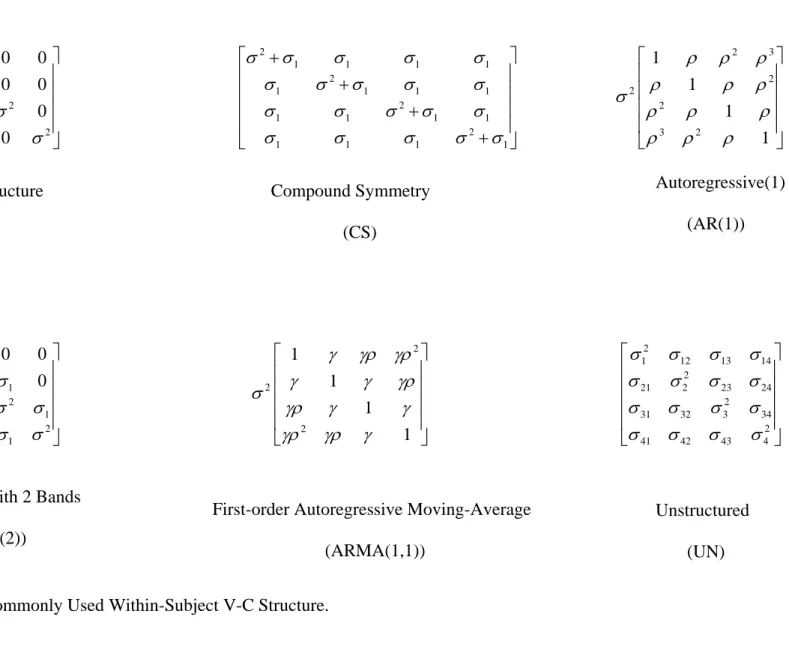
Though MLM has the flexibility in modeling different types of variance-covariance structure, the default V-C structure in popular statistical packages (e.g. HLM, SPSS Mixed, SAS Proc MIXED, and STATA XTMixed) is still the identity structure (i.e. ) where the variance for all the repeated measures is the same and no covariance exists among repeated measures. Assuming no covariance among repeated measures is unrealistic as assuming static covariance in UANOVA with repeated measures. In the following section, commonly used variance-covariance structures in longitudinal data are introduced with the specification on the structures. According to Wolfinger (1993), a wide variety of V-C structures as an alternative to the identity structure can be used for repeated measures. These V-C structures include first-order autoregressive, banded, unstructured, Toeplitz, banded Toeplitz, and first-order autoregressive plus a diagonal. In this section, selected V-C structures are introduced and compared with an illustration of the V-C structures presented in Figure 1.

(27)

14 2 2 2 2 0 0 0 0 0 0 0 0 0 0 0 0                 2 1 1 1 1 2 1 1 1 1 2 1 1 1 1 2 1 1 1 1                         _        _    2 3 2 2 2 3 2 1 1 1 1                          2 1 2 1 1 2 1 1 2 1 0 0 0 0 0 0                       2 2 2 1 1 1 1                          2 1 12 13 14 2 21 2 23 24 2 31 32 3 34 2 41 42 43 4                            

Figure 1. Commonly Used Within-Subject V-C Structure.

Autoregressive(1) (AR(1)) Compound Symmetry (CS) Identity Structure (ID)

First-order Autoregressive Moving-Average (ARMA(1,1))

Unstructured (UN) Toeplitz with 2 Bands

(28)

2.4.1 Identity Structure (ID)

The ID structure specifies that repeated measures are independent for each individual and have homogenous variance. The correlation function between all pairs of lags equals zero. Repeated measures under the ID structure assumption are unrealistic because it assumes no correlation among observation within an individual, though the default V-C structure for most of the popular statistical packages is the identity structure. In terms of equation (5), the ID structure says G=0 and R= , where is an identity matrix.

2.4.2 Compound Symmetric (CS)

The compound symmetric model specifies that individuals have homogeneous variance and homogeneous covariance among observations. The correlations were the same between any pairs of lags within an individual. There are two ways to specify a CS structure in terms of G and R in equation (5), either G= and R= or G=0 and R= , where J is a matrix of ones (Littell et al., 2000).

2.4.3 First-Order Autoregressive (AR(1))

AR(1) specifies the V-C structure to have homogeneous variance but covariance decreasing at an exponential rate with the increase of lags. The AR(1) can be presented as , where is the predicted score at taken at time t, is the error associated with the measurement at time t, is the autocorrelation coefficient,

. “AR models represent the most recent observation in a series as a function of previous observations within the same series.” (Murphy & Pituch, 2009).

(29)

16

2.4.4 First-Order Autoregressive Moving Average Model (ARMA(1,1))

The ARMA(1,1) model is similar to the AR(1) model with the inclusion of an additional moving average parameter, . The ARMA(1,1) model with lag-1 process can be represented as . Like the AR(1) model, )).

ARMA(1,1) specifies the V-C structure to have homogeneous variance and covariance decreasing at an exponential rate of the autocorrelation coefficient plus a multiplicative moving average constant with the increase of lags.

2.4.5 Toeplitz (TOEP)

“Toeplitz structure, sometimes called „banded‟, specifies that covariance depends only on lag, but not as a mathematical function with a smaller number of parameters.” (Littell et al., 2000). TOEP structure specifies the V-C structure to have homogenous variance and mirrored equal covariance along the same band. In terms of equation (5), TOEP structure is specified with G = 0, elements in main diagonal of R are , and for elements in the sub-diagonal, where

with k equal to the row number and l the column number (Littell et al., 2000).

2.4.6 Unstructured (UN)

Unstructured V-C matrix is the most general/unconditional form of V-C structure. Every unique element in the UN V-C structure is estimated with the upper triangle mirroring the lower triangle. In SAS PROC MIXED, the variance is constrained to be non-negative and the covariance is unconstrained (SAS Institute, 2008).

(30)

2.5 Effect of Misspecifying the Within-Subject V-C Structure and Types of Misspecification

Researchers have studied the effect of misspecifying the error structure in repeated measure data in the MLM context (Ferron et al., 2002; Kwok et al., 2007; Murphy & Pituch, 2009; Vallejo et al., 2008). Misspecification in the covariance

structure generally reflected in negative influences on the estimates of standard errors for the fixed effects (Davis, 2002; Diggle, Heagerty, Liang, & Zeger, 2002; Kwok et al., 2007; Singer & Willett, 2003) and the associated hypothesis tests and caused biased statistical inferences or inflated type I error rate and lowered statistical power depending on the types of misspecification (Kwok et al., 2007; Murphy & Pituch, 2009; Vallejo et al., 2008). However, fixed effect estimate and its corresponding hypothesis test remained unbiased for most of the occasions (Ferron et al., 2002). Additionally, misspecification or no specification of the V-C structure may risk the potential of losing information of the change in the outcome variable over time that is reflected only in the covariance matrix of the within-subject residuals (Hedeker & Mermelstein, 2007).

Kwok et al. (2007) defined three types of misspecification in the covariance structure, over-specification, under-specification, and general-misspecification. Over-specification refers to misOver-specification of a simpler covariance structure to a more complex nested structure, for example, misspecifying an identity structure (ID) to a first-order autoregressive structure (AR(1)). On the contrary, under-specification means mis-identifying a more complex covariance structure to a simpler nested structure, for example, incorrectly specifying autoregressive moving average structure (ARMA(1,1))

(31)

18

to AR(1). General misspecification applies to misspecifying covariance structures between two non-nested covariance structure such as misspecifying ID to a banded toeplitz structure (TOEP(2)). Under-specification or general-misspecification often led to overestimation of the random effects and the corresponding standard errors while over-specification may lead to underestimation of the random effects and standard errors (Kwok et al., 2007). Though the effect of misspecification in the covariance structure has been researched, most of the studies only examined misspecification in the side within-subject covariance structure (Ferron et al., 2002; Kwok et al., 2007; Murphy & Pituch, 2009; Vallejo et al., 2008). No research to date has examined the

misspecification in both the between- and within-subject covariance structure simultaneously.

2.6 Selecting an Optimal V-C Structure

Littell et al. (2000) suggested four steps in modeling a mixed effect analysis. Step 1: Model the mean structure by specifying the fixed effects to ensure

unbiasedness of the fixed effect estimates

Step 2: Specify the covariance structure, between subjects as well as within subjects

Step 3: Use GLS estimation method to fit the mean model accounting for the covariance structure

Step 4: Make statistical inference based on the results of step 3 and make the mean model parsimonious

(32)

As a matter of fact, before proceeding from step 3 to step 4, there is an additional inexplicit step, that is, the model selection step for an optimal V-C structure. Researcher should choose among several competing V-C structures to determine which better accounts for the current data under the same mean model. Traditional model selection procedure involves using information criteria such as Akaike Information Criterion (AIC; Akaike, 1974) or Bayesian/Schwartz Information Criterion (BIC; Schwarz, 1978) and likelihood ratio test (LRT). A brief description about the traditional model selection methods was provided along with a potential alternative for searching the optimal V-C structure.

2.6.1 Likelihood Ratio Test (LRT)

Models with nested structures can be evaluated using the likelihood ratio test. The likelihood ratio test is the difference of the deviance statistics between one model nested in another. The deviance statistic is defined as -2 times the ratio of the log-likelihood statistic of the hypothesized model to the log-log-likelihood statistic of the saturated model: Deviance = Hypothesized model Saturated model Log-likelihood 2 Log-likelihood       ₍₆₎

It quantifies the degree of badness of fit (to the data) of the current

(hypothesized) model in comparison to the saturated model. Likewise, we can compute deviance statistics for nested competing models, one with simple covariance structure and the other with more complex structure (e.g. Dsimple & Dcomplex), and obtained a

(33)

20

models. This difference in the deviance statistics between nested models is termed the likelihood ratio test (LRT), which follows a chi-square distribution with degrees of freedom equal the difference between the total parameters estimated in each model. If the test statistic exceeds the value in the chi-square distribution associated with a specific alpha level of significance, we conclude that the simpler model (hypothesized model) is statistically worse than the more complex model and favor the complex model.

Nevertheless, this hypothesis test can only reveal the difference but not magnitude of the difference between the two nested models. Moreover, model selection based on the standard significance test of the nested models is very sensitive to slight deviation between the nested models and tends to over-reject the parsimonious model when the sample size is large (Kuha, 2004).

2.6.2 Akaike Information Criteria (AIC)

AIC can be used for comparing non-nested covariance structures, for example, comparison between banded toeplitz (TOEP(2)) and first order autoregressive and moving average structure, (ARMA (1,1)). The formula for AIC can be written as the following expression:

AIC = d+2k (7) where d is the deviance statistic and k is the number of parameters estimated. Smaller AIC is the-better statistic because smaller values indicate better fit of the model to the data. AIC penalizes additional parameters to be estimated and the size of penalty is 2 multiplied by k.

(34)

2.6.3 Bayesian Information Criteria (BIC)

BIC is also used for non-nested models in comparing covariance structures. The formula for BIC can be represented as:

BIC = d+k*ln(N) (8) where d is the deviance statistic, k is the number of estimated parameters, ln is the natural log, and N is the sample size. Like AIC, smaller BIC is also the-better statistic and penalizes for additional estimated parameters. BIC and AIC differ in the size of penalty, which is k multiplied by ln(N) for BIC. Therefore, BIC usually favors models with fewer parameters (Weakliem, 2004).

Unlike LRT, AIC and BIC quantify the degree of improvement for a given model over a comparison model (O'Connell & McCoach, 2008). However, the results of

empirical studies showed that the accuracy of using these information criteria in search of an optimal covariance structure is not very promising. For example, AIC can

accurately identify the true covariance structure 47% of the time while for BIC is only 35% (Keselman, Algina, Kowalchuk, & Wolfinger, 1998). Research is needed in finding an optimal fit statistic or index that can better determine the appropriate V-C structure for the data.

(35)

22

2.6.4 Standardized Root Mean Square Residual (SRMR)

A possible indicator that can be used for indentifying the true covariance

structure is the standardized root mean square residual (SRMR; Bentler, 1995). SRMR is one of the absolute fit indices that evaluates how well a model reproduces the sample data under the SEM framework (Hu & Bentler, 1998). SRMR is defined as:



  

2 1 1 ˆ 2 SRMR ( 1) t i ij ij ii jj i j s s s T T       _ _ _   _ _       



(9) where s_ij is an element (e.g., the covariance between the ith and jth time points) in the observed/unconditional covariance matrix, ˆijis the corresponding element from the

model-implied covariance matrix based on a specific model, s_iiand s_jjare the observed standard deviations of the ith and jth time points respectively. T is the number of repeated measures in longitudinal data analysis.

According to the algebraic definition, SRMR is a measure of the averaged difference of the standardized residuals between the observed/unconditional and model-implied covariance matrices (Bentler, 1995). SRMR is most sensitive to detecting misspecification in factor covariances (Hu & Bentler, 1998) and is a commonly reported fit index in SEM studies. We can obtain a similar SRMR under the MLM framework. Firstly, we need to confirm and estimate the fixed effect part or the mean model. Once we define a reasonable means model, the unstructured within-subject covariance

structure can be treated as the unconditional covariance matrix because it represents the most general form of the covariance structure. With the same means model, we can

(36)

specify the predicted/model-implied covariance matrix. The SRMR under the MLM framework can then be calculated based on these two covariance matrices. The

effectiveness and performance of SRMR in searching for the optimal V-C structure has, however, not yet been evaluated.

2.7 Discussion

Through the review in the field of multilevel modeling, two research issues are emergent and draw our attention. First, there is a lack of an optimal model selection method, and second the effect of different types/levels of misspecification has not been investigated. Misspecification of the within-subject V-C structure, although it may not have a negative influence on the fixed effect estimates, it can be expected to lead to biased estimation of the standard errors for the fixed effects. In other words, the

statistical inferences drawn from the combination of unbiased fixed estimates and biased standard error of the fixed effects will still be erroneous. The first issue is to develop effective methods for selecting an optimal within-subject V-C structure. Research can be conducted to assess efficacy of traditional fit statistics and evaluate in comparison the proposed SRMR index in selecting the optimal V-C structure.

Second, the misspecification on the R-side of the V-C structure has been

extensively researched (Ferron et al., 2002; Kwok et al., 2007; Murphy & Pituch, 2009; Vallejo et al., 2008). Nevertheless, misspecification in both the G-side (between-subject) and the R-side (within-subject) covariance structures has rarely been examined

simultaneously. In a simple linear growth curve model, the G matrix is comprised of random effects, including variance of intercept ( ), variance of slope , and

(37)

24

covariance between intercept and slope ( ), capturing the deviation of growth

parameters in individuals from the population means for intercept and slope as shown in equation (2). Therefore, whden fitting a mixed effect model for repeated measurements, researchers need to specify both the G- and R- side V-C structure for the data. In the best scenario, researchers will specify the V-C structures for the two sides correctly. In other cases, researchers may over-, under-, or generally misspecify the V-C structures. Research will thus be conducted to investigate the effect of different types/levels of misspecification in both the G and R side V-C matrices, considering the estimation of growth parameters, their standard errors, Type I error rate of the fixed effects, and the empirical statistical power so that we can have a general guideline as to the impact of different types/levels of misspecification on the interpretation of MLM studies.

(38)

3. SEARCHING FOR THE OPTIMAL WITHIN-SUBJECT COVARIANCE STRUCTURE IN LONGITUDINAL DATA ANALYSIS USING MULTILEVEL

MODELING (MLM): A MONTE CARLO STUDY 3.1 Theoretical Framework

Multilevel linear modeling (MLM) is widely used in educational research because many educational data are in a multilevel structure (e.g., repeated measures nested within students and students nested with schools). MLM has also been adopted for analyzing longitudinal data (e.g. repeated measures nested within students) not only because it can capture the average growth trend of the outcome variable over time but also can flexibly model the within-subject covariance structure. However, when analyzing longitudinal data, researchers generally impose the simplest within-subject covariance structure, the identity structure:R=



2I, which is the default structure of the within-subject covariance matrix in many MLM related programs such as HLM, SAS PROC MIXED, SPSS MIXED, and STATA XTMIXED. This within-subject covariance structure is not realistic for longitudinal data because the repeated measures tend to correlate with each other over time and the correlations between measures tend to diminish as the lags in time increase (Hedeker & Gibbons, 2006). Failure to model an appropriate error covariance structure results in: 1) bias estimation of the standard errors of the fixed effects (Davis, 2002; Diggle et al., 2002; Kwok et al., 2007; Singer & Willett, 2003) and 2) the potential of losing information of the change in the outcome variable over time that is reflected only in the covariance matrix of the within-subject residuals (Hedeker & Mermelstein, 2007).

(39)

26

The impact of misspecifying the within-subject covariance matrix has been examined (Ferron et al., 2002; Kwok et al., 2007) and the importance of obtaining the correct covariance structure has been addressed (Singer & Willett, 2003). However, only a few studies (e.g., Keselman et al., 1998; Wolfinger, 1993) have examined the

performance of the traditional methods including the likelihood ratio test (LRT) and the information criteria (e.g., Akaike Information Criteria (AIC) and Bayesian Information Criteria (BIC)) on searching for the correct covariance structure under the mixed model framework. The purpose of this study is to evaluate the performance of these traditional methods on searching for the correct within-subject covariance structure in longitudinal data analysis under the MLM framework. Additionally, a new alternative, standardized root mean square residual (SRMR), is proposed and its performance on searching for the correct covariance structure is compared with the traditional methods.

In this study, the performance of LRT, AIC, BIC, and SRMR on searching for the correct within-subject covariance structure were evaluated. The impact of several factors including sample size, magnitude of the average growth model, and magnitude of the between-subject covariance matrix on the performance of these search methods were also considered in the analysis.

3.2 Method

In this study, we focused on a common two-level growth model with level-1 modeling the repeated measures within individuals and level-2 modeling the differences of individual growth models between individuals. The level 1 and level 2 models can be written as the following expressions:

(40)

2 0 1 Level 1: Y_ti  _i_itime_tie_ti, e_ti ~N(0, ) Level 2: ₀_i ₀₀u₀_i, ₁_i ₁₀u₁_i (10) with 0 00 01 1 10 11 0 ~ , 0 i i u N G u                            

where Y_ti , the personal trajectory of change, is a function of time (time_ti e.g.

ti

time repeated measurement time points) in level one with i indicates individuals, i = 1, ..., N; and t indicates time points, 4 waves: T = 1.5, 0.5, 0.5, 1.5 or 8 waves: T = 3.5, -2.5, -1.5, -0.5, 0.5, 1.5, -2.5, 3.5 centered to have a mean of 0 and 1 unit between adjacent observations. The level two outcome variables, ₀_i (intercept) and ₁_i (slope) are the growth parameters in a linear growth model. ₀_i and ₁_i are multivariate normally distributed and vary around their grand means (₀₀and ₁₀ ) with variance ( ₀₀ and ₁₁) ) and covariance (₀₁ ). We limited our focus to a simple linear growth model with correctly specified fixed effects collected in a balanced design.

3.2.1 Research Design and Model Parameterization

The simulation used a 2 (30 or 210 cases) x 2 (4 or 8 waves) x 3 (magnitude of growth parameter β1: 0, .05 or .16) x 2 (G matrix: small or medium) x 4 (true R matrices

for generating the data: ID, TOEP(2), AR(1), or ARMA(1,1)) factorial design to

generate the data. A total of 500 replications were generated for each condition using the Mplus (V4.1) Monte Carlo procedure (Muthén & Muthén, 1998), yielding 48,000 total datasets. All data were generated under Mplus with a multivariate normal distribution (Muthén & Muthén, 1998). Each dataset was then analyzed using five separate

(41)

28

specifications of the R matrix (ID, TOEP(2), AR(1), ARMA(1,1) and UN) using SAS PROC MIXED (Littell et al., 2006)yielding a total of 240,000 records (i.e., 48,000*5).

For the number of participants, we chose 30 as a “small” number of individuals and 210 as a “medium” number of individualsbased on past simulation studies (Ferron et al., 2002; Keselman et al., 1998) and the review of the multiwave longitudinal studies published in Developmental Psychology by Khoo, West, Wu, & Kwok (2006).

Additionally, we chose 4 waves as the small number of repeated measures and 8 waves as the medium number of measures based on the same review by Khoo and colleagues (Khoo et al., 2006). Three different magnitudes of the standardized effect size of the growth trajectory were examined in this study, no effect (i.e., β1 = .00), small effect size

(i.e., β1 = .05) and medium effect size (i.e., β1 = .16). The standardized effect size is

calculated with the following equation (Raudenbush & Liu, 2001):

11 1     (11) where δ is the standardized effect size, β1 is the average linear growth, and τ11 is

the variance of the random effect associated with the growth, which captures the differences between individual growth trends and the average growth trend. The size of τ11 were set at .05 and .10, where τ11 = .05 is recognized as small and τ11 =.10 as medium

according to Raudenbush and Liu (2001). Given the values of β1 and τ11, the

corresponding δ could be easily computed and the resulting effect size in our simulated data is consistent with small effect size (i.e., δ = .20) and medium effect size (i.e., δ = .50) proposed by Cohen (1988). We also included the size of G matrix (small versus

(42)

medium) as a design factor. According to the criteria provided by Raudenbush and Liu (2001), a medium G and a small G could be specified as:

.200 .050 R .050 .100 Medium        and .100 .025 R .025 .050 small       .

The final design factor to be specified is the true within-subject covariance structure. Four covariance structures, namely, ID, AR(1), TOEP(2), and ARMA(1,1) were adopted in our study. The four within-subject covariance structures are commonly used when analyzing longitudinal data. AR(1) and ARMA(1,1) are commonly

considered in time series analysis (Velicer & Fava, 2003; West & Hepworth, 1991). TOEP(2) is closely related to the moving average (1) structure which is also commonly used in time series analysis. 2 was set as 1 for all the ID, AR(1), TOEP(2), and

ARMA(1,1) models, which is a common practice in power analysis under MLM studies (Bosker, Snijders, & Guldemond, 2003). The autoregressive parameter was set as 0.8. The Toeplitz parameter, 1 , for TOEP(2) and the moving average parameter,  , for ARMA(1,1) were set as 0.5. These values were within the reasonable range of prior studies (Hamaker, Dolan, & Molenaar, 2002; Sivo & Willson, 2000).

3.2.2 Selection Criterion for the Optimal Covariance Matrix

The hit rate (i.e., the percentage of replications with correctly specified within-subject covariance structure) of each search method was used as the major outcome variable. For AIC and BIC, a correct hit in model selection was represented by an event that the smallest AIC or BIC value for the hypothesized covariance structure matches the true covariance structure. AIC and BIC hit rate for all investigated conditions and

(43)

30

correct identification in selecting a true covariance structure was determined in two stages. Firstly, LRT was conducted between the model with a hypothesized covariance structure and the model with the unstructured covariance (UN-structured) structure to examine whether the hypothesized model is statistically worse than the saturated model. If the results are statistically significant for the four hypothesized covariance structures (i.e., the UN-structured covariance fit the data best), there is no need to proceed to the second stage given that LRT fails to select the true covariance structure. Otherwise, cases that did not have a significant LRT proceeded to the second stage, indicating that the hypothesized models do not fit statistically worse than the saturated model. We computed the change in the deviance statistics between pairs of nested competing

covariance structures and performed the chi-square differential test to determine whether the selected covariance structure matched the true covariance structure. After these steps, we calculated the overall hit rate for LRT.

To be selected as the optimal V-C structure for SRMR, two criteria must be met, (1) a SRMR value equal or less than 0.08 and (2) a matching target within-subject covariance matrix. For example, if ARMA(1,1) is the true within-subject covariance structure, one observation has a SRMR value less 0.08 and a target ARMA(1,1) covariance matrix, then SRMR succeeds in selecting the optimal within-subject V-C structure. The 0.08 criterion was selected as suggested by Hu and Bentler (1999) for the cutoff value of SRMR. The hit rate for LRT, AIC, BIC, and SRMR were compared as to their performance on searching for the correct covariance structure.

(44)

3.3 Result

The 2 (30 or 210 cases) x 2 (4 or 8 waves) x 3 (magnitude of growth parameter β1: 0, .05 or .16) x 2 (G matrix: small or medium) factorial design yielded 24 simulation

settings. The 24 settings were named through Model A to Model X. All condition investigated had an UN-structured T matrix with a simulated R matrix which is ID, TOEP(2), AR(1), or ARMA(1,1). The unconditional model for calculating SRMR had an unstructured within-subject variance covariance matrix with Null G so as to avoid model overparametization.

3.3.1 Convergence Rate

The average convergence rate across 24 models was 95%. The result from the ANOVA test suggested convergence rate was moderated by both number of case, number of wave, and their interaction effect (F(3, 20) = 548.603, p < .001). Models with 30 cases and 4 waves had the lowest mean convergence rate (mean = 0.90). Models with 210 cases and 8 waves had the highest mean convergence rate (mean = 0.99), followed by models with 30 cases and 8 waves (mean = 0.97) and models with 210 cases and 4 waves (mean = 0.96).

3.3.2 AIC and BIC Hit Rate

The AIC hit rate is shown in Table 1. The hit rate for a specific within-subject covariance matrix is shown by columns. The hit rate across all within-subject covariance matrices within a certain model is presented by rows. For ID covariance structure, the AIC statistic was able to correctly classify the covariance structure 68% of the time. For TOEP(2), the AIC hit rate was 72%. AR(1) covariance structure had an AIC hit rate of 65%. However, the AIC hit rate decreased to 41% for a true ARMA(1,1) covariance

(45)

32

structure. The overall AIC hit rate across all conditions and within-subject covariance structures was about 62%. The BIC hit rate is presented in. For ID covariance structure, the BIC hit rate reached 84%, for TOEP(2) within-subject covariance 80%, for AR(1) 72%, and for ARMA(1,1) 28%. The overall BIC hit rate across all conditions and within-subject covariance structures was 66%. Analysis of variance (ANOVA) was conducted for both information criteria. The ANOVA test result is presented in Table 3. The 2statistic, the semipartial 2reported in SAS Proc GLM effect size option, was used to evaluate the impact of design factors on the hit rate. The semipartial 2 is the proportion of total variation accounted for by the effect being tested, i.e. the ratio of observed sum of squares due to the effect being tested and the total corrected sample sum of squares. Number of cases (F(5, 18) = 455.37, p < .01) and number of waves (F(5, 18) = 1094.39, p < .01) were both significant factors for the hit rate of AIC. Number of waves alone accounted for 70% of the total variance in the AIC hit rate and number of cases explained the remaining 29% of the between factor variation. Models with 210 cases had a higher AIC hit rate (69.17%) than those with 30 cases (53.42%). Models with 8 waves (73.50%) had a higher AIC hit rate than those with 4 waves (49.08%).

(46)

33 Table 1. AIC Hit Rate

Correct Classification (%) Model # of cases # of waves Magnitude of growth parameter T

matrix ID TOEP(2) AR(1) ARMA(1,1) Average n Convergence

A 30 4 0.00 Medium 58 46 39 9 38 1784 89 B 30 4 0.00 Small 55 52 40 12 40 1802 90 C 30 4 0.05 Medium 58 48 41 13 40 1795 90 D 30 4 0.05 Small 60 58 39 14 43 1802 90 E 30 4 0.16 Medium 57 51 37 15 40 1809 90 F 30 4 0.16 Small 54 55 40 14 41 1815 91 G 30 8 0.00 Medium 73 85 77 32 67 1947 97 H 30 8 0.00 Small 73 82 76 37 67 1953 98 I 30 8 0.05 Medium 73 82 76 36 66 1935 97 J 30 8 0.05 Small 73 79 77 38 67 1940 97 K 30 8 0.16 Medium 73 82 78 32 66 1947 97 L 30 8 0.16 Small 70 79 75 43 66 1947 97 M 210 4 0.00 Medium 71 74 60 31 59 1923 96 N 210 4 0.00 Small 67 65 64 29 59 1915 96 O 210 4 0.05 Medium 73 75 63 26 59 1925 96 P 210 4 0.05 Small 63 60 66 32 55 1936 97 Q 210 4 0.16 Medium 70 74 67 29 60 1915 96 R 210 4 0.16 Small 63 63 63 33 55 1913 96 S 210 8 0.00 Medium 78 82 79 83 81 1974 99 T 210 8 0.00 Small 74 81 81 85 80 1971 99 U 210 8 0.05 Medium 77 84 81 83 81 1973 99 V 210 8 0.05 Small 73 82 80 83 80 1978 99 W 210 8 0.16 Medium 73 83 79 83 80 1973 99 X 210 8 0.16 Small 74 85 80 86 81 1966 98 Total 68 72 65 41 62 45838 95

(47)

34 Table 2. BIC Hit Rate

Correct Classification (%) Model # of cases # of waves Magnitude of growth

parameter T matrix ID TOEP(2) AR(1) ARMA(1,1) Average n Convergence

(48)

The magnitude of the growth parameter (2_{= .0001) and}G matrix (2_{= .0001)} rarely explained any variance in the hit rate of AIC. The hit rate for BIC had similar ANOVA result as the AIC hit rate. Only number of cases and number of waves were significant factors. They accounted for 98% of the variation in BIC hit rate (number of waves, 69%; number of cases, 29%). The 210-case models had a higher BIC hit rate (73.67%) than the 30-case models (56.67%). Likewise, 8-wave models (78.33%) had higher a BIC hit rate than the 4-wave models (52.00%).

3.3.3 SRMR Hit Rate

Table 4 presents the SRMR hit rate. The Matlab codes for calculating SRMR hit rate are presented in Appendix A. The overall SRMR hit rate was 81% across all

investigated conditions and within-subject covariance structures. Correct classification of ID structure was 91%, while the TOEP(2) structure had the highest SRMR hit rate, 92%. AR(1) and ARMA(1,1) had lower SRMR hit rates, 79% and 61% respectively. ANOVA tests were conducted to examine the effect of number of cases, number of waves, magnitude of growth parameter, and G matrix on the hit rate of SRMR.

(49)

36

Table 3. Four-Way Analysis of Variance for AIC and BIC Hit Rate

AIC hit rate BIC hit rate

Factor levels M SD F (5, 18) M SD F (5, 18) n # of cases 455.37** 0.2904 313.16** 0.289 -30 53.42 13.71 56.67 15.05 22476 -210 69.17 11.94 73.67 12.7 23362 # of waves 1094.39** 0.698 751.42** 0.6935 -4 49.08 9.33 52 10.39 22334 -8 73.5 7.33 78.33 7.69 23504 Magnitude of growth parameter 0.05 0.0001 0.21 0.0004 0 61.38 16.08 64.75 17.36 15269 -0.05 61.38 15.24 65.25 15.59 15284 -0.16 61.13 15.53 65.5 16.73 15285 T matrix 0.11 0.0001 0.48 0.0004 - Medium 61.42 15.56 65.5 17.01 22900 - Small 61.17 14.95 64.83 15.99 22938 **p < .0001 for two-tailed test.

2

(50)

37

Table 4. SRMR Hit Rate

Correct classification (%) Model # of cases # of waves Magnitude of growth parameter T matrix

ID TOEP(2) AR(1) ARMA(1,1) Average n Convergence

(51)

38

The result of ANOVA test is shown in Table 5. Like the ANOVA test for AIC and BIC, magnitude of growth parameter and G matrix had small F values and hardly contributed to the variation in the SRMR hit rate. Number of cases (F(5, 18) = 503.05, p < .01) and number of waves cases (F(5, 18) = 76.16, p < .01) were significant factors in the hit rate for SRMR. However, unlike AIC and BIC, number of cases was the largest factor and explained 84% of the variance in SRMR hit rate while number of waves accounted for 13% of the variability in the SRMR hit rate. In the same vein, models with 210 cases (92%) had a higher hit rate than models with 30 cases (69.08%). Eight-wave models (85%) had higher hit rate than 4-wave models (76.08%).

3.3.4 Likelihood Ratio Test

The hit rate of LRT was investigated in four conditions only due to complexity of the two-stage process in selecting the optimal within-subject covariance structure. The overall correct classification was 69% as shown in the bottom of Table 6. The ID within-subject covariance structure had an average hit rate of 91% in LRT, TOEP(2) 93%, and AR(1) 75%. The drop in the LRT hit rate in AR(1) was due to the sharp decrease of the LRT hit rate in the condition with 30 cases and 4 waves, which was 34%. The

(52)

As we took a closer examination of the LRT hit rate for ARMA(1,1), the 210-case and 8-wave combination design had the highest LRT hit rate, 65%. The simulation design condition of 30 cases and 4 waves setting for ARMA(1,1) had only a 1% hit rate. The two remaining design combinations had 0% LRT hit rate. On average, the 210-case and 8-wave combination design had the highest average LRT hit rate (85%) across all within-subject covariance structures.

Table 5. Four-Way Analysis of Variance for SRMR Hit Rate

SRMR hit rate Factor levels M SD F (5, 18) n # of cases 503.50** 0. 8363 -30 69.03 3.42 22476 -210 92.00 6.66 23362 # of waves 76.16** 0.1266 -4 76.08 10.06 22334 -8 85.00 14.07 23504 Magnitude of growth parameter 0.41 0.0013 0 80.50 12.98 15269 -0.05 80.00 13.93 15284 -0.16 81.13 13.23 15285 T matrix 3.52 0.0058 - Medium 79.58 13.65 22900 - Small 81.50 12.41 22938

**p < .0001 for two-tailed test.

2

(53)

40

Table 6. LRT Hit Rate

Correct classification (%) Target Σ Matrix # of cases # of

waves ID TOEP(2) AR(1) ARMA(1,1) Average n

ID 30 4 92 55 2367 TOEP(2) 30 4 92 2996 AR(1) 30 4 34 2861 ARMA(1,1) 30 4 1 2583 ID 210 4 91 69 2567 TOEP(2) 210 4 96 3000 AR(1) 210 4 91 3000 ARMA(1,1) 210 4 0 2960 ID 30 8 93 65 2680 TOEP(2) 30 8 87 3000 AR(1) 30 8 83 3000 ARMA(1,1) 30 8 0 2989 ID 210 8 89 85 2835 TOEP(2) 210 8 96 3000 AR(1) 210 8 90 3000 ARMA(1,1) 210 8 65 3000 Total 91 93 75 17 69 45835