Working Paper No. 2009-26
Constructing consumer Sentiment
Index for U.S. Using Internet Search
Patterns
Nicolás Della Penna
Haifang Huang
University of Alberta
October, 2009
Copyright to papers in this working paper series rests with the authors and their assignees. Papers may be downloaded for personal use. Downloading of papers for any other activity may not be done without the written consent of the authors.
Short excerpts of these working papers may be quoted without explicit permission provided that full credit is given to the source.
The Department of Economics, The Institute for Public Economics, and the University of Alberta accept no responsibility for the accuracy or point of view represented in this work in progress.
Constructing Consumer Sentiment Index for
U.S. Using Google Searches
by
Nicolás Della Penna
Data analyst London, UK [email protected] and
Haifang Huang
Assistant professor Department of Economics, University of Alberta, Edmonton, Alberta, T6G 2H4 Canada [email protected].Keywords: macroeconomics; consumer spending; consumer confidence; time series; forecast; internet searches.
JEL classifications: E21, E27, C53.
Acknowledgement: We thank Rick Szostak, Linda Nøstbakken, Harper Reed and Garrett Johnson for their helpful comments and contributions.
Note: The following paper is the draft posted on RePEc through the UoA Economics Working Paper Series in October, 2009. A February, 2010 revision is available upon request from the authors. We thank Henry van Egteren for his comments during that revision.
Constructing Consumer Sentiment Index for U.S. Using Google Searches Nicolás Della Penna and Haifang Huang1
October 2009
(Comments welcome)
Abstract:
We construct a consumer sentiment index for the U.S. using the popularity trends of selected Google searches. The final index consists of four components and is highly correlated with the Index of Consumer Sentiment from the University of Michigan and the Consumer Confidence Index from the Conference Board. Among the three sentiment indices, the Google search-based index (SBI) leads in time and predicts other indices. In terms of forecasting consumer spending, the SBI outperforms both the ICS and the CCI and provides independent information. For robustness, we use multiple measures of consumer spending and a range of statistical specifications. The finding is robust. 1. Introduction
About 70 percent of the U.S. GDP is personal consumption. Variations in consumption are an important part of the business cycle in the country. Consumption also reflects the population’s expectations; its variations thus have forecasting value. As a result, the release of consumption data in the U.S. can affect the stock market. A recent example is the weaker-than-expected retail sales announced in July 2009. The stock market dropped after the data release, despite the upbeat assessment by the Federal Reserve on the economy. A headline on MSNBC.com declared: “On Wall Street, Shoppers Trump the Fed.”2
Economic forecasters have developed various sentiment indices to keep track of
consumers’ willingness to spend. In the U.S., the two major indices are the University of Michigan’s Index of Consumer Sentiment (ICS) and the Conference Board’s Consumer Confidence Index (CCI). They are survey-based measures that are intended to gauge consumers’ confidence in the economy. The monthly release of these indices also affects markets. For example, after the August 2009 release of the ICS, two article titles on Bloomberg.com read: “Euro Tumbles as U.S. Consumer Confidence Outweighs Region's GDP,” and “German Stocks Drop as U.S. Consumer Sentiment Unexpectedly Falls.”
1
Della Penna is a computational economist based in London, UK; Huang is an assistant professor of economics at the University of Alberta, Canada. For inquiries about the paper, please email
[email protected] and [email protected].
2
Associated Press, http://www.msnbc.msn.com/id/32438282/ns/business-stocks_and_economy/; updated 11:59 a.m. MT, Sun., Aug. 16, 2009.
We believe variations in Internet search patterns also reflect consumer sentiment. There are two reasons for our view. First, some people use the Internet to look for or research products they want to purchase; changes in search patterns should thus reflect changes in demand. We believe certain demands reveal consumers’ purchasing power and
confidence (for example demand for luxury goods). Second, people use the Internet to research issues that concern them, such as debt burden and energy costs, both of which could affect consumers’ purchasing power.
In this paper we construct a consumer sentiment index for the U.S. using the popularity trends of selected Internet searches on Google. The selection reflects our hypotheses about the causes and the symptoms of changes in the sentiment. We test these hypotheses using data from inside and from outside the U.S.: from the U.S. we use a panel of 49 states; from outside the country we use a panel of Canadian provinces and another panel of advanced economies. We regress consumption-related dependent variables on the Google search series. Only searches that have the hypothesized sign in all three panels are included in the final index.
We construct the final index as the unweighted sum of its standardized components of Internet searches; each component is signed (positive or negative) but is otherwise treated equally. We interpret changes in the popularity of these components of Internet searches as a reflection of changes in, respectively, personal financial condition, business climate, consumers’ willingness to spend on discretionary items, and the public’s concern about energy costs.
The search-based index (SBI) has correlation coefficients of 0.9 with the two survey-based indices (the ICS and CCI). It provides statistically significant information for predicting other indices, but other indices cannot predict the SBI. When it comes to forecasting consumer spending, the SBI generally outperforms the other two indices. Finally, the index has a unique and important advantage: the underlying data from Google Insights are free and are available on a weekly basis, as opposed to monthly. We thus recommend the index as a major measure of consumer confidence, for its timeliness, availability, and simplicity of construction.
We are not aware of other papers that use Internet searches to measure consumer sentiment. The inspiration for our project came from Choi and Varian (2009), who use information from Google searches to forecast sales in motorcycles, auto insurance, trucks and SUVs, several brands of automotives, as well as home sales. Our paper’s objective is different. We want to construct a consumer sentiment index at the aggregate level, and evaluate the effort by comparing the resulted index to existing sentiment indices. Other papers that use Google searches in economics or finance studies include Da, Engelberg, and Gao (2009), who find that stocks that experience higher search volume have
“stronger price momentum,” and Askitas and Zimmermann (2009), who find “strong correlations between keyword searches and unemployment rates using monthly German data.”
Among earlier works, our paper is related to the literature that examines the ICS and CCI for forecasting purposes. Carroll, Fuhrer, and Wilcox (1994) find that “lagged values of the ICS … explain … variations in the growth of total real personal consumption
expenditures.” Howrey (2001) confirms the finding and further observes that “the ICS is a useful recession indicator variable.” His finding echoes an earlier one by Matsusak and Sbordone (1995) that the “hypothesis that consumer sentiment does not cause GNP (in the Granger sense) can be rejected.” Bram and Ludvigson (1998) conducted a horse race between the ICS and the CCI. They find the CCI to “have both economically and
statistically significant explanatory power for several spending categories,” while the ICS “exhibits weaker forecasting power.” Our paper does not take a position regarding the relative power of the ICS and CCI, but compares the SBI to the ICS and CCI together.
The structure of the paper is as follows: In section 2 we explain the nature of the Google data. In section 3 we explain how we select the Google searches, stating our underlying hypotheses and testing them using the three panels from the U.S., Canada, and other advanced economies. In section 4 we explain why we want to use equal weights instead of estimation-based weights in the construction of our index. In section 5, we examine the dynamic relationship between the search-based index and the survey-based indices (the ICS and the CCI); we also compare these indices in their information content in
predicting consumer spending. Section 6 concludes.
2. Google Insights for Search and its measure of popularity of searches
Through Google Insights for Search, Google has made available the information on its users’ Internet search patterns. According to the company, the data enable the public to “compare search volume patterns across specific regions, categories, time frames and properties.” The data do not reflect absolute volume; instead they reflect popularity, or “the likelihood of users in a particular area to search for a term on Google on a relative basis,” in Google’s words. More specifically, when Google’s data show that the term “hotel” is equally popular in Canada and Fiji, it does not mean the absolute volume of searches is the same. Rather, it means that “users in both Fiji and Canada are equally likely to search for the term ‘hotel.’”
The data we choose to use in this paper have been further normalized by initial
popularity. The initial value (usually the first week of January 2004) is always zero, and subsequent data points measure percentage growth of the popularity measure with respect to the first date.3 A positive (negative) value for “hotel” in September 2005 means
Google users were more (less) likely to search for “hotel” in September 2005 than they were in January 2004; the numerical value reflects the difference in percentage points of the initial popularity measure.4
3
For more information, please refer to Google Help > Insights for Search Help > Working with Insights for Search > Analyzing Data. URL: http://www.google.com/support/insights/bin/topic.py?topic=13975.
4
Google does not clarify its exact formula, but we believe it is along the lines of x_t = [ln(searches for “x” at time t/total searches at time t) - ln(searches for “x” at time 0/total searches at time 0)] *100%.
Google has classified its users’ Internet searches into categories. A few examples of the categories or subcategories include “Shopping > Luxury Goods,” “Society > Legal > Bankruptcy,” “Science > Ecology,” “Recreation > Hobbies > Paintball,” and “Society > Government & Regulatory Bodies > Visa & Immigration.”
We use Google’s categories to construct our index of sentiment. All the data we use are at the categorical (or sub-categorical) level, as opposed to the keyword level. We download the data from http://www.google.com/insights/search/#.
Google Insights provides data at a weekly frequency. This means the index based on Google searches can be updated every week, as opposed to having to wait for the monthly releases of the ICS and CCI. In an effort to utilize this unique advantage, we construct our index to ensure that it is always available before the release of CCI. The release date for the CCI is usually in the last week of the current month, the earliest date being the 24th. We choose the cutoff date of the Google-based index to be the week before the 24th, so that the index always becomes available before the CCI. For example, our April 2009 index is aggregated from Google searches made between March 22, 2009 and April 18, 2009. The release date of the CCI for that month was April 28, so our index preempts the CCI by 10 days in this case. The ICS is released on the 15th of each month, so our index mostly falls between the release of the ICS and the release of CCI.
Finally, the time series of many Google searches clearly exhibit seasonal patterns. For this reason we seasonally adjust the Google data using monthly dummies. Specifically, we regress the time series of individual categories of Google searches onto eleven monthly dummies and a linear time trend. We then subtract from the original time series values that are equal to the estimated coefficients on corresponding monthly dummies. We use the adjusted time series for our analysis.
3. The selection of search categories for the search-based sentiment index
Our index of consumer sentiment will use the popularity trends of selected categories of Google searches. We start our selection by trying to ensure correspondence with the questions in the ICS survey, but precise correspondence is not possible. To a greater extent, the selection reflects our hypotheses about the causes and the symptoms of changes in consumer confidence, and how they may manifest themselves in Internet searches.
We do not have enough existing literature on Internet searches to guide the selection procedure. Instead, we seek to verify our hypotheses using three panels of data.
Specifically, we collect consumption-related variables at the state level in the U.S., at the provincial level in Canada, and at the national level for several other advanced
economies. We then regress the consumption variables onto the candidate categories of Internet searches. Our criterion for selection, admittedly ad hoc, is that we only use categories that have the hypothesized signs in predicting immediate and future changes in consumption across all three panels.
The U.S. panel consists of 48 states plus D.C.. It uses changes in retail trade as a proxy for changes in consumer spending, because monthly consumption or retail sales data are unavailable for most states. The Canadian panel consists of three large Canadian
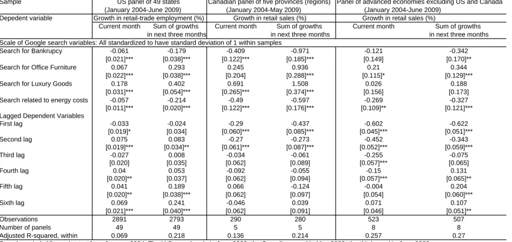
provinces and two regions that lump together the remaining seven smaller ones. For this Canadian panel we do have the data on retail sales. The panel of advanced economies consists of eight countries: Japan, Germany, France, the United Kingdom, Italy, Austria, the Netherlands, and Sweden. These are the entire set of International Monetary Fund (IMF)-defined “advanced economies,” for which retail sales data are available from the Organisation for Economic Co-operation and Development (OECD) and for which Google information is available at the categorical level.5 All panels start from January 2004, since that is when the Google data start. The panel’s termination dates are determined by the availability of retail data: the U.S. panel ends in June 2009, the Canadian panel ends in May 2009, and the eight-country panel ends in June 2009. Our final selection consists of only four categories. Table 1 presents the results from six regressions that test the direction of co-movements between the selected Internet searches and consumption. We have six regressions because there are three panels and two
dependent variables for each: one of the dependent variables is the current change in the consumption variable; the other is the change during the next three months.
[Insert Table 1 here]
We interpret the first category as a reflection of adversarial financial conditions. It is what Google defines as “Society > Legal > Bankruptcy.” Personal financial conditions are a principal focus of the ICS survey. It asks its respondents: “Would you say that you (and your family living there) are better off or worse off financially than you were a year ago?” Google searches do not allow direct measurement of Internet users’ evaluation of their financial conditions. We hypothesize, however, that rising interest in the legal terms of bankruptcy indicates rising burden of debt, and thus a worsened condition. The sign of the coefficients of this category shown in Table 1 are all negative, suggesting that
populations in the U.S., Canada, and other economies search more about bankruptcy at times when they reduce their consumption. Our interpretation is that the populations become more concerned about bankruptcy in financially difficult times. We
experimented with another search category: “Finance & Insurance > Credit & Lending > Debt Management.” It is rejected because it attracts a positive sign in the OECD panel. One possible explanation is that interest in debt management could arise from prudence and indicate pending demand for loans: a prudent household should research how to manage debt if they are planning to obtain a loan in order to finance a large purchase. The category does attract negative coefficients in the U.S. and in Canada, though.
We interpret our second selected category, “Business > Office & Printing Services > Office Furniture,” as a measure of business conditions. We want to incorporate business
5
For the list of “advanced economies,” please refer to the World Economic Outlook 2009 published by the IMF at http://www.imf.org/external/pubs/ft/weo/2009/01/weodata/groups.htm#ae. Google provides search information for many countries, but not all of them have information at the level of categories. The database of the OECD statistics can be accessed through http://stats.oecd.org/Index.aspx.
conditions into the index of consumer sentiment because we expect the former to affect the target of the measurement. Both the University of Michigan and the Conference Board ask their survey respondents to evaluate business conditions in their sentiment surveys.6 Unlike those surveys, ours does not try to measure the population’s opinion about business conditions; we hope to approximate the condition itself. We choose “office furniture” because furniture is a durable investment. We hypothesize that some of the demand for office furniture comes from newly established or soon-to-be-established offices. The search interest therefore provides information about the current and future pace of business investment. The remainder of the demand comes from existing offices. We think that this type of demand is likely to increase during prosperous times. Since furniture is durable, its services can be prolonged if businesses do not wish to spend money on immediate upgrades. Rising demand for furniture from existing offices thus indicates business confidence. The regression results reported in Table 1 is consistent with out hypothesis: the coefficient on this category in explaining the immediate and future changes in consumption is consistently positive across all panels.
We use a third category, “Shopping > Luxury Goods,” to capture households’ willingness to spend on discretionary items. Luxury goods are chosen for their discretionary nature. Historically, sales of luxury goods have been highly correlated with the performance of the stock market, much more so than aggregate consumption (Ait-Sahalia, Parker, and Yogo, 2004). Sales dropped sharply in 1970, 1974, 1991, and 2001, coinciding with contraction phases of the business cycle. We hypothesize that demand for luxury goods reflects positive consumer sentiments, and that Internet searches reflect the demand for these goods. The results in Table 1 lend support to the hypothesis: coefficients on
“Luxury Goods” are positive in all six regressions. We experimented with another search category, “Home and Garden > Home Furnishing.” The rationale for choosing home furnishing is similar to that for choosing office furniture: furniture is durable, so the demand for it is likely to increase when consumers fell more confidence of their financial situations. The U.S. state-level panel indeed assigns positive coefficients to this category. But the Canadian provincial panel and the eight-country national panel both produce the opposite signs. We thus excluded the category from the final index.
We use a fourth category to measure the population’s attention to energy costs. Large fluctuations in energy costs have been common in the U.S. since 1973. Rising gasoline prices and heating bills in the winter tend to attract significant attention from news media and from politicians.7 Many economists are also concerned about the impact of rising energy costs on consumption. For example, in 2006 the Federal Reserve chairman Bernanke (Bernanke, 2006) stated that “an increase in oil prices slows economic growth in the short run primarily through its effects on consumer spending ... [T]he cumulative increase in imported energy costs since the end of 2003 … [a]ll else being equal …
6
The University of Michigan survey asks what the respondents think about the “business conditions in the country as a whole.” The Conference Board survey asks the respondents to “rate present general business conditions” as well as the conditions six months from now.
7
The winter of 2007-08 saw more than a few reports of elderly found dead in unheated or underheated residences. The media generally linked these incidents to the high cost of heating. As for gasoline prices, two major U.S. presidential hopefuls in 2008, John McCain and Hillary Clinton, proposed gas tax holidays as a response to rising prices.
constitutes a noticeable drag on real household incomes and spending.” A study by Doms and Morin (2004), which does not focus on energy costs, finds that changes in the price of gasoline attract a negative coefficient in explaining the University of Michigan’s measure of consumer sentiment.Their empirical model controls for many important variables of economic conditions. We thus interpret the still-negative coefficient of gasoline prices as an indication that energy costs are important to consumer confidence.8
We originally use the popularity of “Industries > Energy & Utilities” to measure the population’s attention to the issue. To check whether this is a reasonable approximation, we examine the popularity data and the level of oil prices during the period: they do appear closely related. The search popularity has two significant peaks: September 2005 and May-July 2008. Oil prices, coincidentally, peaked on both occasions.9 We also look at the leading search keywords that Google lists under this category. These keywords include “energy,” “oil,” “solar,” “gas prices,” and “oil prices.” But they also include “waste management” and “recycling,” which do not appear to have direct connection to the cost of energy. For this reason, we go to the subcategorical level. We keep three of the four subcategories — “Oil & Gas,” “Electricity,” and “Alternative Energy” — but replace the one that is called “Waste Management” with “Automotive > Hybrid & Alternative Vehicles,” the interest in which is likely to fluctuate with gasoline prices as well. We then combine the four sub-components back into a single category using an un-weighted mean of standardized scores. In the regressions in Table 1, the category attracts negative coefficients in all panels, for both immediate and future changes in
consumption.
The following table presents the categories used in the index and their expected signs in parentheses. These signs are drawn from the estimated coefficients reported in Table 1.
1. Adversarial financial conditions (-)
a. Category: Society > Legal > Bankruptcy 2. Business conditions (+)
a. Category: Business > Office & Printing Services > Office Furniture 3. Willingness to spend on discretionary items (+)
a. Category: Shopping > Luxury Goods 4. Attention to energy costs (-)
a. A synthetic category: the sum of standard scores of i. Industries > Energy & Utilities > Oil and Gas ii. Industries > Energy & Utilities > Electricity
iii. Industries > Energy & Utilities > Alternative Energy iv. Automotive > Hybrid & Alternative Vehicles
8
Doms and Morin (2004)’s effort is to understand the relation between information flow and the formation of consumer sentiment. Other economic variables in their empirical model include changes in S&P prices, CPI, unemployment rate, and payroll employment. Their main interest is in the news media’s coverage and tone of economic reporting.
9
Oil price was at $60 a barrel in September 2005, rising from $34 in January of the same year, and started to fall after September. The price peaked again at $133 in July 2008. The price data can be found on the website of the U.S. Energy Information Administration, Department of Energy; URL:
4. The construction of the index
We need to combine various categories into a single index. The purpose is to reduce dimensions while retaining important information, making the resulting index easier to present. Both the University of Michigan and the Conference Board use a similar strategy: their overall indices of consumer sentiment are aggregated from five survey questions.
We propose to assign equal weights to each category (in a standardized scale) to construct the final index. The primary motivation is simplicity; we also want to follow the precedent of the Composite Leading Economic Index, which is an unweighted sum of 10 components, constructed by the Conference Board in the U.S. and by Statistics
Canada. The alternative is to use estimation-based weights. That, as demonstrated by Auerbach (1982), raises concerns about the stability of the weights.
We conclude this section by presenting the exact formula of the final index. The search-based index is denoted as SBI. On the right-hand side of the formula, std() indicates standardized scores:
SBI = - std(Bankruptcy) + std(Office Furniture) + std(Luxury Goods) -
[0.25*std(Energy & Utilities) + 0.25*std(Electricity) + 0.25*std(Alternative Energy) + 0.25*std(Hybrid & Alternative Vehicles)]
5. The search-based consumer sentiment index for the U.S.
Our purpose is to construct an index of consumer sentiment for the U.S. based on Internet searches. We denote the resulting index as the SBI, or search-based index. In this section we will examine the correlation and lead-lag relationship between the SBI and two survey-based indices: the University of Michigan’s Index of Consumer Sentiment (ICS), and the Conference Board’s Consumer Confidence Index (CCI). We will test whether the SBI predicts the ICS and CCI, and whether the SBI predicts consumer spending. We will then compare the SBI’s information content to that of the ICS and CCI.
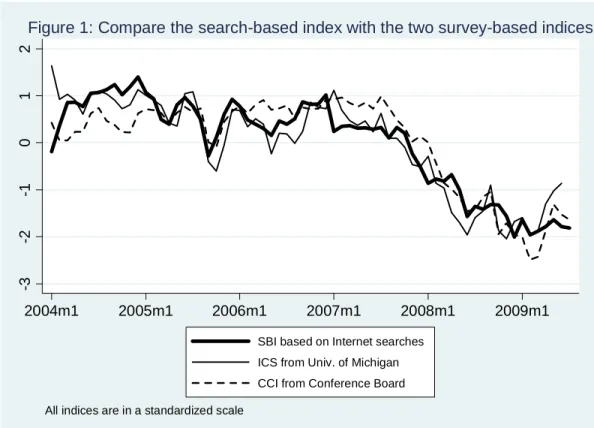
5.1. Dynamic relation between the search-based index and the survey-based indices Table 2 shows the bivariate correlation coefficients between the SBI and the two survey-based indices (the ICS and CCI). They are approximately 0.9, similar to the correlation between the ICS and CCI themselves.
Table 2: Correlation coefficients between the search-based index (SBI), the Conference Board’s Consumer Confidence Index (CCI), and the University of Michigan’s Index of Consumer
Sentiment (ICS)
SBI CCI ICS
SBI 1
CCI 0.90 1
ICS 0.91 0.89 1
Figure 1 presents a plot of these three sentiment indices. Given the high correlations, it is not surprising that all three indices follow similar trajectories.
[Insert Figure 1 here]
To investigate the lead-lag relationship between the indices, Table 3 presents the correlation coefficients between changes in the SBI and the lead, the lagged, and the current changes in the ICS and CCI.
Table 3: The lead, lag, and contemporaneous correlations between changes in the search-based index (SBI) and changes in survey-based indices (the ICS and CCI)
Last-month Current-month Next-month
changes in CCI changes in CCI changes in CCI
Changes in SBI -0.21 0.43 0.20
Last-month Current-month Next-month
changes in ICS changes in ICS changes in ICS
Changes in SBI -0.04 0.38 0.29
Sample period: monthly data between January 2004 and June 2009 (July 2009 for CCI).
The contemporaneous correlations between changes in the SBI and changes in the other two indices are approximately 0.4, and these correlation coefficients are statistical different from zero given the sample size. More interestingly, the correlation between changes in the SBI and future changes in the ICS and CCI are positive, but the correlation between lagged changes in the ICS (or CCI) and current changes in the SBI is negative. This suggests the SBI leads the ICS and CCI in time. The finding suggests that one could try using the SBI to predict survey-based indices, which is what we do in Tables 4 and 5. Table 4 presents a forecast model for changes in the University of Michigan’s ICS. When the model uses six lags of the dependent variable, its adjusted R2 is 0.1. The adjusted R2 rises to 0.19 once we add one lagged change of SBI as an additional predictor. The null hypothesis that the SBI variable has no information content is rejected at below the 1% level of significance. Furthermore, the SBI appears to be a better predictor than another survey-based index - the CCI by the Conference Board – in forecasting ICS, because the adjusted R2 is smaller if we replace the lagged change in SBI with the lagged change in CCI.
Table 4: Using the search-based index (SBI) to predict changes in the University of Michigan’s ICS
Predicting changes in ICS
with six lags of DV Adj_R2=0.10
with six lags of DV & one lagged change of SBI Adj_R2=0.19
The sum of coefficients of the six lagged DV -0.46
The coefficient of the lagged change in SBI 0.36
p-value against the null that the SBI can be excluded 0.004
Replacing the lagged change in SBI with that in CCI Adj_R2=0.17
Note: The dependent and the independent variables (month-to-month changes in this table) are standardized to have a Stdev of 1 in the sample. Hypothesis tests use heteroskedasticity-and-serial-correlation-robust covariance matrix. Sample period: monthly data between January 2004 and June 2009.
Table 5 presents the forecast model for changes in the CCI. Using lagged changes as sole predictors generates a miserable fit. Adding the lagged changes in the SBI marginally improves it. The SBI information, however, has a p-value less than 10%. Furthermore, the SBI can take comfort from the fact that it performs better than the ICS in predicting the CCI. The model that uses the ICS to predict the CCI has an even worse fit.
Table 5: Using the search-based index (SBI) to predict changes in the Conference Board’s CCI
Predicting changes in CCI
with six lags of DV Adj_R2=-0.06
with six lags of DV & one lagged change of SBI Adj_R2=-0.04
The sum of coefficients of the six lagged DV -0.20
The coefficient of the lagged change in SBI 0.24
..p value that the SBI can be excluded 0.09
Replacing the lagged change in SBI with that in ICS Adj_R2=-0.07
Note: The dependent and the independent variables (month-to-month changes in this table) are standardized to have a Stdev of 1 in the sample. Hypothesis tests use heteroskedasticity-and-serial-correlation-robust covariance matrix. Sample period: monthly data between January 2004 and July 2009.
Finally, for comparison, Table 6 reports results for the model that uses changes in the CCI and ICS to predict changes in the SBI. In both cases, the null of no information cannot be rejected. This confirms the timing advantage of search-based indices, since the SBI predicts the survey-based indices, while the survey-based indices do not predict SBI. This suggests that one can potentially use Internet searches to develop an
advance-warning system that would indicate changes in the economy earlier than consumer surveys.
Table 6: Using changes in survey-based indices (the ICS and CCI) to predict changes in the search-based index (SBI)
Predicting changes in SBI
with six lags of DV Adj_R2=0.15
with six lags of DV & one lagged change of ICS Adj_R2=0.14
..p value that the ICS can be excluded 0.80
with six lags of DV & one lagged change of CCI Adj_R2=0.16
..p value that the CCI can be excluded 0.22
Note: The dependent and the independent time series (month-to-month changes in this table) are standardized to have a Stdev of 1 in the sample. Hypothesis tests use heteroskedasticity-and-serial-correlation-robust covariance matrix. Sample period: monthly data between January 2004 and June 2009 (July 2009 for CCI).
The following summarizes the key findings in this section:
1. Simple correlations: In terms of their levels, the SBI, ICS, and CCI are highly correlated with 0.9 correction coefficients. In terms of month-to-month changes, the SBI and the survey-based indices are moderately correlated; the correlation coefficients are about 0.4.
2. Lead-lag relation: The SBI leads the ICS and CCI, not the other way around. Changes in the SBI have statistically significant information in predicting changes in the ICS and CCI, especially for the ICS.
3. Comparison: the SBI is a slightly better predictor of the CCI than the ICS; it is a slightly better predictor of the ICS than the CCI.
5.2. Dynamic relationship between the search-based index and consumer spending The objective of measuring consumer sentiment is to provide a timely indicator of consumer confidence and spending. None of the indices would be interesting if they failed to predict consumptions. This section tests whether the search-based index provides information about future consumption and whether it provides better information than the two survey-based indices. We use retail sales and Personal
Consumption Expenditure (PCE), both in real terms, as measures of consumer spending. First we look at simple correlations. Table 7 presents the bivariate correlation coefficients between the monthly growth of consumer spending (measured by retail sales and PCE) and the three sentiment indices. It describes the correlation coefficients between the level of sentiment and the changes in consumption, as well as those between the changes in sentiment and the changes in consumption. In all cases, the SBI exhibits stronger correlation with future consumer spending than its survey-based competitors. The advantage is more obvious in the case of change-to-change correlations.
Table 7. Bivariate correlation coefficients between consumption growth and the search-based index (SBI), the survey-based indices (the ICS and CCI), and their changes
Next-month growth in retail sales in Personal Consumption Expenditure Level of SBI 0.33 0.40 Level of ICS 0.32 0.34 Level of CCI 0.26 0.32 Changes in SBI 0.30 0.28 Changes in ICS 0.11 0.12 Changes in CCI 0.02 0.08
Sample period: All series start from January 2004. SBI and CCI end in July 2009, ICS and retail sales in June 2009, PCE in May 2009.
In the next step we formally test the predictive power of the sentiment indices. We use three different statistical specifications for the purpose. Here we describe these
specifications. All three can be found in relevant literature; some take extra measures to guard against the possibility of unit roots.
The first specification uses the lagged level of sentiment indices to predict the growth in consumer spending. It is well known in this literature that the correlation between the level of sentiment and the change in consumption is high (see, for example, Figure 1 of Carroll, Fuhrer, and Wilcox, 1994). The level-to-growth specification can be found in Carroll, Fuhrer, and Wilcox (1994) and Bram and Ludvigson (1998). Both papers test whether consumer sentiment indices forecast household spending. Carroll, Fuhrer, and Wilcox (1994) use the ICS, while Bram and Ludvigson (1998) compare the CCI against the ICS.
The second specification uses changes in the sentiment indices to predict changes in consumer spending. This specification, although for a different purpose, can be found in Auerbach (1982). The purpose of Auerbach (1982) is to test the power of the Composite
Leading Economic Index in predicting future unemployment rates and industrial
production in the U.S. There is a benefit from using differences, as opposed to levels, in our exercise: it reduces the likelihood that the correlations are spurious because of unit roots. The presence of a unit root in the sentiment indices means non-stationarity. We do not believe the indices are non-stationary, but Dickey Fuller tests fail to reject the
presence of unit roots for all of the three indices. We think the result is due to the boom-to-bust episode in the sample period. In any case, because of the inability of Dickey Fuller tests to reject unit roots, we use the first difference of the indices for our predictions. Dickey Fuller tests strongly reject unit roots in these first differences, including the first difference of the search-based index.
For these two specifications, we include six lags of the dependent variable and six lags of growth in real personal disposable income as control variables. The growth in disposable income is included because the dependent variable is the change in consumption, and there could be correlation between lagged income and consumption that is not completely captured by lagged consumptions.
The last specification is an error-correction model with consumption, disposable income, and the sentiment indices. Howrey (2001) uses this specification to examine the
predictive power of the ICS for monthly growth of personal consumption expenditure. This specification provides an additional robustness test.
The following three equations describe the exact specifications. In all these equations C is either the retail sales or the personal consumption spending; the term Y is the disposable income; the term S is the consumer sentiment indices (the SBI, CCI or ICS).
Specification 1: t i i t i i i t i i i t i t const C Y S u C
6 1 6 1 6 1 ˆ ln ˆ ln ˆ ln Specification 2: t i i t i i i t i i i t i t const C Y S u C
6 1 6 1 6 1 ˆ ln ˆ ln ˆ ln Specification 3: t t t t t t t t const C C Y Y S S u C ln ˆ1 ln 1 ˆ2ln 1 ˆ1 ln 1 ˆ2ln 1 ˆ1 1 ˆ2 1Table 8 presents results from 18 regressions. The number 18 comes from the fact that we have two alternative dependent variables, three alternative specifications, and three alternative sentiment indices. For each regression, Table 7 shows the adjusted R2; for the regression that uses the search-based index, the table also provides the p-value for the null hypothesis that it has no information at all (ie. the joint hypothesis that all
coefficients of SBI variables are zero). Finally, the table also shows the adjusted R2 for the model without any sentiment index at all, which allows us to observe the increments in adjusted R2 due to the inclusion of sentiment indices.
Table 8. Testing and comparing the forecasting power of the SBI against the two survey-based indices (the ICS and CCI)
Without With sentiment information
sentiment ICS CCI SBI #
Adj.R2 Adj.R2 Adj.R2 Adj.R2 p-value that SBI Of
D.V. can be excluded Obs
Spec. 1 D.log.RetailSales 0.11 0.30 0.11 0.34 0.000 59 D.log.PCE 0.09 0.29 0.10 0.34 0.000 58 Spec. 2 D.log.RetailSales 0.11 0.11 0.10 0.23 0.002 59 D.log.PCE 0.09 0.18 0.14 0.22 0.002 58 Spec. 3 D.log.RetailSales 0.08 0.14 0.17 0.26 0.000 64 D.log.PCE 0.15 0.24 0.23 0.29 0.002 63
Sample period: All series start from January 2004. Retail sales end in June 2009, PCE in May 2009. All sentiment indices cover June 2009.
Here is a summary of the observations we make from Table 3:
1. The null that the SBI has no information in predicting consumer spending is strongly rejected in all cases at below 1%.
2. The SBI outperforms either the two survey-base indices in all cases in terms of adjusted R2.
3. The average contribution of the SBI to the adjusted R2, from the model without sentiment at all, is 0.24 in the first specification, 0.125 in the second specification, and 0.16 in the third one.
The appendix presents detailed regression results for interested readers. Here we simply want to state that the lagged levels and lagged changes of the SBI are always positive whenever they are present in the predictive models. This means that higher levels in the SBI and/or positive movements of the SBI always mean higher growth rates in
consumption. There are no unexpected signs as far as the SBI is concerned.
The next table, Table 9, asks whether the SBI outperforms the combined force of the two survey-based indices. It also asks whether the SBI contributes any independent
information when both the ICS and the CCI are included in the forecasting model. To answer the first question, we compare the forecast accuracy (in terms of adjusted R2) between the forecast model that uses the SBI only and one that uses both ICS and the CCI. To answer the second question, we test the joint hypothesis — in a model that uses SBI, ICS, and CCI — that all the SBI variables’ coefficients are zero.
Table 9. Comparing the SBI’s information content to the combined force of the CCI and ICS
SBI ICS & CCI ICS & CCI & SBI #
Adj.R2 Adj.R2 Adj.R2 p-value that SBI Of
(as in Table 8) can be excluded obs
Spec. 1 D.log.RetailSales 0.34 0.28 0.46 0.001 59 D.log.PCE 0.34 0.18 0.44 0.000 58 Spec. 2 D.log.RetailSales 0.23 0.22 0.38 0.004 59 D.log.PCE 0.22 0.19 0.28 0.048 58 Spec. 3 D.log.RetailSales 0.26 0.19 0.30 0.000 64 D.log.PCE 0.29 0.24 0.27 0.076 63
Sample period: All series start from January 2004. Retail sales end in June 2009, PCE in May 2009. All sentiment indices cover June 2009.
Table 9 shows that the SBI outperforms the ICS and CCI combined: in all comparisons the SBI achieves a higher adjusted R2 than the ICS and CCI together. It also shows that the SBI adds independent information to that provided by the two other indices, because in all tests the null of no independent information is rejected, at below 10% in one case, and at below 5% for the other five cases.
6. Conclusion
As the Internet becomes a part of daily life, people use it to search for information about issues and items that interest or concern them. It follows that by keeping track of
aggregate search patterns, one can keep an eye on the public’s interests and concerns. This paper offers one example of using search data for such purposes. We construct a consumer sentiment index for the U.S. based on changes in search patterns that are recorded and made available to the public by Google Insights.
Our search-based index of consumer sentiment (SBI) is based on the popularity of four categories of Google searches: “Society > Legal > Bankruptcy,” “Business > Office & Printing Services > Office Furniture,” “Shopping > Luxury Goods,” and a synthetic category that combines information from “Industries > Energy & Utilities” and “Automotive > Hybrid & Alternative Vehicles.” We interpret changes in the search patterns in the four categories as a reflection of adversarial financial conditions, healthy business conditions, consumers’ willingness to spend on discretionary items, and public concern about energy costs, respectively. Furthermore, we show that all four categories of searches have the hypothesized signs in three mutually exclusive and wide-ranging panels of data: the U.S. state-level panel, the Canadian provincial panel, and an
advanced-economy panel excluding the U.S. and Canada. Finally, we construct the SBI as the unweighted sum of the standardized scores of the four categories’ popularity trends.
We find a correlation coefficient of 0.9 between this index and the two major survey-based indices of consumer sentiment: the University of Michigan’s Index of Consumer Sentiment (ICS) and the Conference Board’s Consumer Confidence Index (CCI). Furthermore, we find that the SBI leads the survey-based indices in time: changes in the SBI predict changes in the ICS and CCI, but those in the CCI and ICS do not predict changes in the SBI.
We also find that the SBI has statistically significant information in predicting growth in Personal Consumption Expenditure (PCE) and retail sales. In fact, the SBI outperforms the CCI and ICS individually and the two of them together. The finding is robust in a range of statistical specifications: prediction based on the level of the sentiment indices, prediction based on changes in the sentiment indices, and prediction based on error correction models.
We thus conclude that the patterns of Internet searches made available by Google Insights can be used to monitor changes in consumer sentiment. The Google data are available on a weekly basis, as opposed to the monthly frequency of the survey-based
indices. Google data thus allow researchers to keep a more timely watch on consumer sentiment.
References
AIT-Sahalia, Yacine & Jonathan A. Parker & Motohiro Yogo (2004). "Luxury Goods and the Equity Premium," Journal of Finance, American Finance Association, Vol. 59(6), pp. 2959-3004, December.
Askitas, Nikos & Zimmermann, Klaus F. (2009). "Google Econometrics and
Unemployment Forecasting," IZA Discussion Papers 4201, Institute for the Study of Labor (IZA).
Auerbach, Alan J. (1982). "The Index of Leading Indicators: Measurement without Theory, Thirty-Five Years Later." The Review of Economics and Statistics, Vol. 64, No. 4 (November 1982), pp. 589-595.
Bernanke, B.S. (2006). “Energy and the Economy,” Speech to the Economic Club of Chicago, June 15.
Bram, Jason & Ludvigson, Sydney (1998). "Does consumer confidence forecast
household expenditure? a sentiment index horse race," Economic Policy Review, Federal Reserve Bank of New York, issue June, pp. 59-78.
Carroll, Christopher D. & Fuhrer, Jeffrey C. & Wilcox, David W. (1994).
"Does Consumer Sentiment Forecast Household Spending? If So, Why?", American Economic Review, American Economic Association, Vol. 84(5), pp. 1397-1408. Choi, Hyunyoung & Varian, Hal (April 2009), "Predicting the Present with Google Trends," http://www.google.com/googleblogs/pdfs/google_predicting_the_present.pdf Da, Zhi & Engelberg, Joseph & Gao, Pengjie (June 4, 2009). "In Search of Attention," Available at SSRN: http://ssrn.com/abstract=1364209.
Doms, Mark & Norman Morin (2004). "Consumer sentiment, the economy, and the news media," Working Papers in Applied Economic Theory 2004-09, Federal Reserve Bank of San Francisco.
Howrey, E. Philip (2001). "The Predictive Power of the Index of Consumer Sentiment," Brookings Papers on Economic Activity, Economic Studies Program, The Brookings Institution, Vol. 32(2001-1), pp. 175-216.
Matsusaka, John G. & Sbordone, Argia M. (1995). "Consumer Confidence and Economic Fluctuations," Economic Inquiry, Oxford University Press, Vol. 33(2), pp. 296-318, April.
Table 1: The direction of co-movement between selected Google searches and growth in consumption-related variables
regression model: Fixed-effect panel regression
Sample US panel of 49 states Canadian panel of five provinces (regions) Panel of advanced economies excluding US and Canada (January 2004-June 2009) (January 2004-May 2009) (January 2004-June 2009)
Depedent variable Growth in retail-trade employment (%) Growth in retail sales (%) Growth in retail sales (%)
Current month Sum of growths Current month Sum of growths Current month Sum of growths
in next three months in next three months in next three months
Scale of Google search variables: All standardized to have standard deviation of 1 within samples
Search for Bankrupcy -0.061 -0.179 -0.409 -0.971 -0.121 -0.342
[0.021]*** [0.038]*** [0.122]*** [0.185]*** [0.149] [0.170]**
Search for Office Furniture 0.067 0.293 0.245 0.936 0.21 0.344
[0.022]*** [0.038]*** [0.204] [0.288]*** [0.115]* [0.129]***
Search for Luxury Goods 0.178 0.402 0.691 1.508 0.026 0.188
[0.031]*** [0.054]*** [0.265]*** [0.374]*** [0.156] [0.173]
Search related to energy costs -0.057 -0.214 -0.49 -0.597 -0.269 -0.327
[0.011]*** [0.020]*** [0.122]*** [0.176]*** [0.109]** [0.121]***
Lagged Dependent Variables
First lag -0.033 -0.024 -0.29 -0.437 -0.602 -0.622 [0.019]* [0.034] [0.060]*** [0.085]*** [0.045]*** [0.051]*** Second lag 0.075 0.083 -0.27 -0.273 -0.452 -0.343 [0.019]*** [0.034]** [0.061]*** [0.087]*** [0.052]*** [0.059]*** Third lag -0.027 0.008 -0.034 -0.061 -0.255 -0.075 [0.020] [0.035] [0.062] [0.089] [0.057]*** [0.065] Fourth lag 0.04 0.053 -0.092 -0.055 -0.15 0.131 [0.020]** [0.037] [0.062] [0.094] [0.057]*** [0.065]** Fifth lag 0.041 0.189 0.066 -0.124 -0.004 0.204 [0.020]** [0.038]*** [0.062] [0.097] [0.054] [0.060]*** Sixth lag 0.069 0.241 -0.046 0.039 0.071 0.107 [0.021]*** [0.040]*** [0.062] [0.091] [0.046] [0.051]** Observations 2891 2793 290 280 523 507 Number of panels 49 49 5 5 8 8
Adjusted R-squared, within 0.069 0.218 0.136 0.214 0.257 0.27
Sample period: All panels start from January 2004. The U.S. panel ends in June 2009, the Canadian panel in May 2009, the third panel in June 2009 *** p<0.01, ** p<0.05, * p<0.1
-3 -2 -1 0 1 2 2004m1 2005m1 2006m1 2007m1 2008m1 2009m1
SBI based on Internet searches ICS from Univ. of Michigan CCI from Conference Board
All indices are in a standardized scale
Appendix Table 1: Predicting monthly growths in retail sales and Personal Consumption Expenditure using specification 1
Model: where std() indicates
standard scores.
When the DV is growth in retail sales When the DV is growth in personal consumption expenditure
L.DV 0.004 -0.253 -0.087 -0.414 -0.116 -0.175 -0.089 -0.409 -0.321 -0.43 -0.46 -0.291 [0.168] [0.152] [0.148] [0.206]* [0.161] [0.143] [0.171] [0.175]** [0.168]* [0.198]** [0.192]** [0.192] L2.DV 0.161 -0.185 -0.048 -0.121 -0.146 -0.059 0.291 -0.07 0.051 -0.015 -0.099 -0.129 [0.203] [0.210] [0.228] [0.186] [0.262] [0.267] [0.219] [0.219] [0.240] [0.235] [0.259] [0.233] L3.DV 0.045 -0.257 -0.116 -0.083 -0.294 -0.134 0.119 -0.183 -0.061 -0.13 -0.169 -0.342 [0.122] [0.165] [0.171] [0.178] [0.182] [0.126] [0.160] [0.188] [0.194] [0.165] [0.210] [0.151]** L4.DV -0.04 -0.268 -0.15 -0.14 -0.216 -0.142 0.117 -0.226 -0.077 -0.118 -0.202 -0.216 [0.144] [0.135]* [0.139] [0.231] [0.165] [0.180] [0.120] [0.168] [0.148] [0.187] [0.215] [0.192] L5.DV 0.153 -0.19 -0.077 -0.323 -0.198 -0.306 0.23 -0.189 -0.028 -0.241 -0.218 -0.406 [0.105] [0.161] [0.120] [0.176]* [0.238] [0.295] [0.102]** [0.191] [0.162] [0.140]* [0.208] [0.208]* L6.DV 0.142 -0.244 -0.046 -0.3 -0.252 -0.329 -0.007 -0.256 -0.21 -0.435 -0.277 -0.519 [0.125] [0.169] [0.164] [0.156]* [0.230] [0.224] [0.115] [0.152]* [0.150] [0.130]*** [0.182] [0.147]*** LD.Y 0.15 0.155 0.137 0.206 0.085 0.136 0.041 0.076 0.077 0.064 0.087 0.025 [0.203] [0.159] [0.168] [0.186] [0.138] [0.133] [0.083] [0.068] [0.080] [0.085] [0.072] [0.061] L2D.Y 0.121 0.166 0.192 0.224 0.12 0.194 -0.042 0.024 0.019 0.018 0.037 0.056 [0.200] [0.158] [0.183] [0.180] [0.160] [0.172] [0.089] [0.083] [0.081] [0.072] [0.085] [0.071] L3D.Y 0.004 0.159 0.118 0.132 0.148 0.114 -0.053 0.032 0.008 0.011 0.04 0.089 [0.171] [0.158] [0.200] [0.180] [0.162] [0.183] [0.068] [0.068] [0.072] [0.077] [0.071] [0.065] L4D.Y 0.123 0.238 0.203 0.245 0.199 0.215 -0.042 0.032 0.006 0.024 0.035 0.088 [0.210] [0.186] [0.205] [0.189] [0.157] [0.145] [0.065] [0.064] [0.076] [0.071] [0.071] [0.049]* L5D.Y -0.295 -0.1 -0.192 -0.102 -0.13 -0.183 -0.158 -0.063 -0.106 -0.058 -0.053 0.011 [0.174]* [0.190] [0.207] [0.171] [0.168] [0.138] [0.064]** [0.076] [0.077] [0.060] [0.081] [0.051] L6D.Y 0.009 0.18 0.091 0.042 0.194 0.004 -0.048 0.014 -0.016 -0.009 0.02 0.012 [0.099] [0.140] [0.153] [0.112] [0.153] [0.085] [0.042] [0.058] [0.065] [0.039] [0.056] [0.046] L.ICS 0.056 0.054 0.026 0.02 0.023 -0.004 [0.025]** [0.044] [0.065] [0.010]* [0.014] [0.018] L2.ICS -0.026 -0.059 -0.032 -0.008 -0.005 -0.001 [0.040] [0.063] [0.033] [0.014] [0.023] [0.019] L3.ICS -0.031 -0.012 -0.001 -0.008 -0.017 0.009 [0.042] [0.078] [0.073] [0.014] [0.022] [0.019] L4.ICS 0.08 0.12 0.107 0.032 0.03 0.046 [0.037]** [0.050]** [0.048]** [0.012]*** [0.016]* [0.020]** L5.ICS -0.02 -0.062 -0.088 -0.014 -0.015 -0.037 [0.037] [0.053] [0.042]** [0.014] [0.017] [0.016]** L6.ICS 0.015 0.038 0.038 0.008 0.013 0.003 [0.022] [0.032] [0.032] [0.009] [0.011] [0.016] L.CCI 0.013 -0.005 -0.019 0.011 0 -0.003 [0.021] [0.035] [0.035] [0.010] [0.013] [0.008] L2.CCI 0.013 0.024 0.081 -0.002 -0.007 0.017 [0.033] [0.038] [0.033]** [0.014] [0.017] [0.017] L3.CCI -0.015 0.003 -0.066 -0.004 0.01 -0.016 [0.042] [0.055] [0.054] [0.012] [0.012] [0.014] L4.CCI 0.004 -0.058 -0.005 0.01 0.001 -0.013 [0.029] [0.031]* [0.035] [0.008] [0.012] [0.014] L5.CCI 0.038 0.053 0.029 0 0.003 0.032 [0.023] [0.035] [0.035] [0.010] [0.012] [0.014]** L6.CCI -0.038 -0.026 -0.027 -0.007 -0.006 -0.015 [0.015]** [0.024] [0.029] [0.007] [0.009] [0.013] L.SBI 0.463 0.555 0.14 0.212 [0.160]*** [0.177]*** [0.054]** [0.075]*** L2.SBI -0.504 -0.905 -0.066 -0.146 [0.119]*** [0.200]*** [0.066] [0.077]* L3.SBI 0.084 0.288 -0.105 -0.169 [0.179] [0.220] [0.053]* [0.086]* L4.SBI -0.068 -0.033 0.135 0.207 [0.180] [0.190] [0.057]** [0.063]*** L5.SBI 0.385 0.158 -0.03 -0.171 [0.228]* [0.266] [0.065] [0.081]** L6.SBI -0.055 0.028 0.055 0.134 [0.142] [0.170] [0.046] [0.075]* Constant -0.08 -6.462 -1.602 -0.459 -6.082 -3.855 0.098 -2.181 -0.487 0.284 -2.172 -1.186 [0.232] [2.439]** [1.205] [0.350] [2.372]** [5.128] [0.063] [0.785]*** [0.417] [0.068]*** [0.931]** [1.646] Observations 59 59 59 59 59 59 58 58 58 58 58 58 Adjusted R2 0.106 0.296 0.113 0.337 0.278 0.462 0.091 0.293 0.103 0.335 0.181 0.44
Standard errors in brackets.
*** p<0.01, ** p<0.05, * p<0.1; Hypothesis tests use heteroskedasticity-and-serial-correlation-robust covariance matrix.
t i i t i i i t i i i t i t const C Y std S u C 6 1 6 1 6 1 ) ( ˆ 100 * ln ˆ 100 * ln ˆ 100 * ln
Appendix Table 2: Predicting monthly growths in retail sales and Personal Consumption Expenditure using specification 2
Model: where std() indicates
standard scores.
When the DV is growth in retail sales When the DV is growth in personal consumption expenditure
L.DV 0.004 0.043 -0.036 -0.15 0.032 -0.007 -0.089 -0.085 -0.218 -0.156 -0.217 -0.007 [0.168] [0.130] [0.151] [0.169] [0.166] [0.123] [0.171] [0.119] [0.139] [0.140] [0.153] [0.159] L2.DV 0.161 0.197 0.072 0.277 0.078 0.269 0.291 0.211 0.126 0.335 0.052 0.246 [0.203] [0.209] [0.206] [0.201] [0.241] [0.247] [0.219] [0.226] [0.219] [0.198]* [0.250] [0.301] L3.DV 0.045 0.057 -0.019 0.18 -0.14 0.076 0.119 0.172 0.04 0.185 0.063 -0.06 [0.122] [0.157] [0.149] [0.149] [0.156] [0.119] [0.160] [0.187] [0.175] [0.139] [0.182] [0.192] L4.DV -0.04 -0.045 -0.095 0.074 -0.059 0.02 0.117 0.201 0.053 0.139 0.149 0.096 [0.144] [0.141] [0.115] [0.164] [0.126] [0.149] [0.120] [0.130] [0.094] [0.139] [0.151] [0.202] L5.DV 0.153 0.134 0.044 -0.04 0.075 -0.119 0.23 0.191 0.142 0.111 0.132 0.067 [0.105] [0.095] [0.129] [0.102] [0.206] [0.240] [0.102]** [0.134] [0.116] [0.087] [0.135] [0.136] L6.DV 0.142 0.065 0.048 -0.017 -0.072 -0.169 -0.007 -0.098 -0.11 -0.134 -0.125 -0.216 [0.125] [0.139] [0.130] [0.112] [0.168] [0.146] [0.115] [0.104] [0.117] [0.116] [0.136] [0.142] LD.Y 0.15 0.095 0.11 0.11 0.085 0.088 0.041 0.026 0.048 0.009 0.052 -0.011 [0.203] [0.178] [0.166] [0.171] [0.134] [0.126] [0.083] [0.072] [0.079] [0.080] [0.065] [0.062] L2D.Y 0.121 0.039 0.157 0.053 0.136 0.1 -0.042 -0.066 -0.005 -0.066 0.007 -0.02 [0.200] [0.172] [0.164] [0.157] [0.176] [0.165] [0.089] [0.078] [0.079] [0.059] [0.088] [0.080] L3D.Y 0.004 -0.027 0.097 -0.115 0.162 -0.036 -0.053 -0.068 -0.001 -0.096 0.016 0.001 [0.171] [0.155] [0.190] [0.149] [0.203] [0.194] [0.068] [0.061] [0.071] [0.061] [0.078] [0.088] L4D.Y 0.123 0.071 0.191 0.032 0.186 0.075 -0.042 -0.083 -0.008 -0.07 -0.018 -0.012 [0.210] [0.200] [0.192] [0.179] [0.167] [0.148] [0.065] [0.056] [0.066] [0.060] [0.065] [0.060] L5D.Y -0.295 -0.318 -0.239 -0.365 -0.221 -0.345 -0.158 -0.172 -0.135 -0.159 -0.122 -0.106 [0.174]* [0.176]* [0.183] [0.141]** [0.151] [0.125]** [0.064]** [0.062]*** [0.063]** [0.054]*** [0.066]* [0.052]* L6D.Y 0.009 0.037 0.039 -0.117 0.123 -0.122 -0.048 -0.036 -0.037 -0.066 -0.012 -0.051 [0.099] [0.127] [0.131] [0.105] [0.129] [0.099] [0.042] [0.053] [0.056] [0.039]* [0.048] [0.054] LD.ICS 0.035 0.036 0.003 0.022 0.022 -0.005 [0.025] [0.047] [0.066] [0.009]** [0.015] [0.023] L2D.ICS 0.012 -0.037 -0.054 0.013 0.011 -0.014 [0.036] [0.085] [0.084] [0.011] [0.021] [0.028] L3D.ICS -0.034 -0.074 -0.074 -0.002 -0.012 -0.014 [0.039] [0.053] [0.067] [0.013] [0.023] [0.023] L4D.ICS 0.043 0.03 0.033 0.024 0.009 0.028 [0.029] [0.043] [0.032] [0.008]*** [0.018] [0.020] L5D.ICS 0.004 -0.062 -0.054 -0.004 -0.026 -0.019 [0.029] [0.040] [0.040] [0.012] [0.013]** [0.019] L6D.ICS 0.015 -0.04 -0.024 0.02 -0.002 -0.01 [0.026] [0.036] [0.044] [0.008]** [0.014] [0.021] LD.CCI 0.001 -0.012 -0.022 0.006 -0.004 -0.005 [0.022] [0.029] [0.031] [0.009] [0.011] [0.009] L2D.CCI 0.023 0.039 0.084 0.011 0.001 0.021 [0.018] [0.050] [0.058] [0.007] [0.014] [0.021] L3D.CCI 0.009 0.05 0.028 0.006 0.011 0.01 [0.027] [0.034] [0.035] [0.008] [0.013] [0.017] L4D.CCI 0.013 0.003 0.015 0.014 0.014 -0.008 [0.019] [0.031] [0.026] [0.008]* [0.014] [0.014] L5D.CCI 0.047 0.065 0.042 0.011 0.024 0.023 [0.019]** [0.029]** [0.028] [0.009] [0.010]** [0.016] L6D.CCI 0.028 0.058 0.014 0.017 0.024 0.014 [0.025] [0.034]* [0.039] [0.008]** [0.011]** [0.014] LD.SBI 0.436 0.595 0.124 0.184 [0.161]** [0.198]*** [0.059]** [0.097]* L2D.SBI -0.069 -0.3 0.092 0.068 [0.127] [0.144]** [0.045]** [0.058] L3D.SBI 0.047 -0.039 -0.025 -0.104 [0.154] [0.191] [0.041] [0.084] L4D.SBI -0.036 0.005 0.091 0.113 [0.139] [0.187] [0.050]* [0.042]** L5D.SBI 0.203 0.089 0.025 -0.038 [0.159] [0.221] [0.050] [0.054] L6D.SBI 0.27 0.18 0.104 0.041 [0.151]* [0.121] [0.053]* [0.047] Constant -0.08 0.007 -0.048 0.126 -0.082 0.099 0.098 0.173 0.223 0.209 0.207 0.232 [0.232] [0.241] [0.242] [0.211] [0.223] [0.196] [0.063] [0.076]** [0.103]** [0.073]*** [0.093]** [0.080]*** Observations 59 59 59 59 59 59 58 58 58 58 58 58 Adjusted R2 0.106 0.109 0.104 0.23 0.216 0.382 0.091 0.182 0.14 0.216 0.193 0.277
Standard errors in brackets.
*** p<0.01, ** p<0.05, * p<0.1; Hypothesis tests use heteroskedasticity-and-serial-correlation-robust covariance matrix.
t i i t i i i t i i i t i t const C Y std S u C 6 1 6 1 6 1 ) ( ˆ 100 * ln ˆ 100 * ln ˆ 100 * ln
Appendix Table 3: Predicting monthly growths in retail sales and Personal Consumption Expenditure using specification 3
Model:
where std() indicates standard scores.
When the consumption measure C is retail sales When C is personal consumption expenditure
LD.C -0.237 -0.33 -0.209 -0.411 -0.202 -0.317 -0.321 -0.454 -0.41 -0.46 -0.423 -0.444 [0.137]* [0.121]*** [0.133] [0.101]*** [0.155] [0.144]** [0.156]** [0.129]*** [0.126]*** [0.110]*** [0.139]*** [0.132]*** L.C -0.001 -0.051 -0.196 -0.085 -0.221 -0.218 0.011 -0.007 -0.078 -0.025 -0.078 -0.06 [0.034] [0.035] [0.062]*** [0.036]** [0.089]** [0.091]** [0.037] [0.046] [0.077] [0.048] [0.117] [0.103] LD.Y 0.155 0.118 0.084 0.056 0.076 0.023 0.084 0.072 0.043 0.047 0.041 0.032 [0.094] [0.101] [0.077] [0.119] [0.065] [0.087] [0.038]** [0.032]** [0.035] [0.029] [0.050] [0.046] L.Y -0.092 -0.006 0.031 0.066 0.012 0.081 -0.052 -0.006 0.053 0.027 0.047 0.048 [0.030]*** [0.060] [0.045] [0.051] [0.051] [0.050] [0.039] [0.052] [0.079] [0.053] [0.101] [0.088] LD.ICS 0.017 0.066 0.059 0.008 0.021 0.019 [0.036] [0.044] [0.039] [0.014] [0.016] [0.016] L.ICS 0.039 -0.018 -0.028 0.013 -0.002 -0.004 [0.022]* [0.043] [0.048] [0.006]** [0.018] [0.016] LD.CCI -0.022 -0.056 -0.068 -0.001 -0.012 -0.015 [0.020] [0.022]** [0.025]*** [0.010] [0.013] [0.012] L.CCI 0.038 0.049 0.039 0.008 0.009 0.006 [0.012]*** [0.026]* [0.026] [0.004]** [0.011] [0.010] LD.SBI 0.264 0.318 0.059 0.071 [0.121]** [0.125]** [0.047] [0.046] L.SBI 0.25 0.187 0.074 0.05 [0.080]*** [0.115] [0.028]** [0.045] Observations 64 64 64 64 64 64 63 63 63 63 63 63 Adjusted R2 0.076 0.142 0.171 0.255 0.19 0.296 0.151 0.237 0.23 0.288 0.238 0.269 Standard errors in brackets.
*** p<0.01, ** p<0.05, * p<0.1; Hypothesis tests use heteroskedasticity-and-serial-correlation-robust covariance matrix.
t t t t t t t t const C C Y Y std S std S u C ln *100 ˆ1 ln 1*100 ˆ2ln 1*100 ˆ1 ln 1*100 ˆ2ln 1*100 ˆ1 ( 1) ˆ2 ( 1)