CHAPTER VII CALCULATING PREMIERSHIP ODDS BY COMPUTER: AN ANALYSIS OF THE AFL FINAL EIGHT PLAY-OFF SYSTEM

CHAPTER VII

CALCULATING PREMIERSHIP ODDS BY COMPUTER: AN ANALYSIS OF THE AFL FINAL EIGHT PLAY-OFF SYSTEM

7.0. Abstract

The Australian Football League's final eight play-off system is explained and the premiership chances of all teams are evaluated and compared with previous final systems. The importance of matches, and the playing order necessary to avoid dead finals is discussed. A computer tipping program published weekly in a daily newspaper produces the probability of any team beating any other team on any ground. This was extended to calculate the chances of every possible finishing order in the finals. The suitability and fairness of the play-offs is evaluated under various criteria. The use of such a program to assist in framing premiership and quinella odds is discussed, and inconsistencies between bookmakers' odds on individual matches and winning the premiership highlighted. Home ground advantage in finals is assessed. It is shown that the knockout nature of the finals magnifies any home advantage possessed by a team.

Key words: sport, football, finals, play-off, probabilities, odds

7.1. Introduction

Australian rules football is the major winter sport of the southern states of Australia. From a base of 12 Melbourne clubs, by 1994 the Australian Football League (AFL) had expanded to 15 teams including teams from Sydney, Brisbane, Adelaide and Perth. The season consists of a 22 game home and away schedule followed by a final series between the top teams culminating in a grand final to determine the premier team. For many years the author has operated a computer program to predict the results of individual games Clarke (1988c, 1991a, 1993b). The predictions are published each week in the daily press and Clarke (1992a) shows that they compare favourably with human tipsters. In addition to selecting the winner of any match, the computer program estimates the chances of either team winning. Near the end of the 1992 home and away series a program was written that would produce, at the beginning and during the final series, each team's chance of winning the grand final. In 1994 this needed updating for the new final eight system introduced by the AFL.

normal knockout system of three matches (two semi-finals and a final) used in most competitions with four finalists, the Page final four gives an advantage to the top teams by introducing a bye and a double chance. The top two teams play, with the winner gaining direct entry into the grand final by virtue of a bye the following week; the loser is not eliminated but has a second chance by playing the winner of the lower two teams for the right to play in the grand final. This became known as 'the double chance'. Thus the top two teams are advantaged by either gaining the bye or receiving the double chance. Over the years, several variations on this theme were used as the number of teams in the finals was increased. In 1972 the league introduced a final five played under the 'McIntyre Final Five' system (see Schwertman & Howard, (1989, 1990)) and in 1991 the AFL introduced a new finals system played between the top six teams. After some criticism, they adjusted the system again for 1992 with the 'McIntyre Final Six' system. As Clarke (1993b) points out, this introduced a controversial aspect into the finals as the path a team takes, and hence its chances of winning the premiership, is determined by the results of matches in which it does not participate. This aspect was entrenched when, for 1994, the Am, introduced the final eight, with a series of nine finals matches over four weeks, called the McIntyre Final Eight system (MF8).

Monahan & Berger (1977), in discussing the fairness of play-off structures in hockey suggest three criteria for measuring their suitability: maximise the probability that the highest ranked team wins, maximise the expected number of points of the premier, and maximise the chance the best two teams meet in the final. In their conclusions they point out that in some of their proposed structures, a lower-ranked team has a higher chance of reaching the semi-final and final than a higher-ranked team, and this is unacceptable to players who are rewarded according to final position. In such competitions (the AFL prize money and the following year's draft are affected by final position), the play-off system should not be judged solely on how fairly it determines the premier, but how fairly it determines all positions. This suggests several other criteria - the probability of a team finishing in any position or higher should be greater than for any lower-ranked team; the expected final position should be in order of original ranking; the probability of a team finishing above a team of lower rank should be greater than 0.5 and should increase as the difference in ranks increases; the probability of any two teams appearing in the grand final should monotonically decrease as the ranks of the two teams increases. To these we might add one of consistency between years - teams of the same ranking that perform in a similar manner in different years should finish in similar positions.

7.2. The McIntyre Final Eight system

The MF8 consists of nine matches: four qualifying finals the first week, two semi-finals the second week, two preliminary finals the third week and the grand final the fourth week. For the first three weeks, two teams are eliminated each week. The original ladder ranking before the finals determines the draw for the first week of the finals, and also determines the relative position of the winners and losers each week.

During week 1, four Qualifying finals are played: lv8,2v7,3v6 and 4v5. This produces four winners who go to the top of the ladder and four losers who go to the bottom. Within these two groups they preserve their original ranking. Thus after week 1, we have a new ranking of Winner 1, Winner 2, Winner 3, Winner 4, Loser 1, Loser 2, Loser 3, Loser 4, although in the following we will usually use the terminology of current ranking one to eight. An example will illustrate. In 1994 the qualifying finals were lv8 West Coast v Collingwood, 2v7 Carlton v Melbourne, 3v6 North Melbourne v Hawthorn and 4v5 Geelong v Footscray.

MF8 week 1 matches from 1994 and resulting week 2 draw

Original ladder ranking 1 2 3 4 5 6 7 8 Team West Coast Carlton North Melb Geelong Footscray Hawthorn Melbourne Collingwood Week 1 Current result ranking win 1- Winner 1 loss 2- Winner 2 win 3- Winner 3 win 4- Winner 4 loss 5- Loser 1 loss 6- Loser 2 win 7- Loser 3 loss 8- Loser 4 Team West Coast North Melb Geelong Melbourne Carlton Footscray Hawthorn Collingwood Week 2 match Bye Bye Semi 2 Semi 1 Semi 2 Semi 1 Eliminated Eliminated

The bottom two teams are eliminated, and from week 2 onwards the system is a knockout tournament with the current top two teams gaining a bye in week 2. Under the old final four, in week 2 one team has a bye straight through to the final in week 3, while two other teams play to see which of them continues. This system is the same but in two halves (teams currently ranked 1, 4 & 6 in one half and teams 2, 3 & 5 in the other). Teams 1 and 2 get a bye straight through to the two preliminary finals in week 3, while 4

two winners of the preliminary finals play in the grand final.

A feature of the MF8 is the degree to which a team's progress depends on results in other matches. One year team 3 could win the first week and not gain the bye, while another year team 6 could win and gain the bye. Similarly team 3 could lose and be eliminated one year whereas another year team 6 could lose but not be eliminated. Under the assumption that all teams are equal, the chances of teams 1 to 8 gaining the bye if they win are respectively loo%, loo%, 75%, 50%, 50%, 25%, 0% and 0%. The same list reversed gives the chances of the teams being eliminated if they lose. This is the first finals system where a team's elimination has depended on other match results.

Note that the positions after the first week are symmetrical. If after the first week a team is now ranked position N, their opponent from the first week will now be in position 9N. Put another way, a team's opponent will be as far off the bottom as the team is from the top. It is easily proved using this symmetry that there can be no repeat finals matches until the grand final since respective opponents from week I go into opposite halves of the draw.

The symmetry also means that the first round opponents of the teams eliminated gain the bye. This implies these two matches were very important to the participants - the winner gained the bye, the loser was eliminated. However it is not known beforehand which of the matches are elimination matches as they are determined by the results in other matches. Thus in the most perverse cases, if both 1 and 2 lose, the 3v6 and 4v5 matches become the elimination matches with 3 and 4 eliminated if they lose and 5 and 6 gaining the bye. On the other hand if 1 and 2 both win, these matches are virtually irrelevant, as the winner cannot gain the bye nor the loser be eliminated. The result merely determines in which semi-finals the four teams will play.

7.3. Premiership chances

-

comparison with previous systems

For the case when all teams are considered equal, the chances of winning the premiership can be calculated easily by first principles. For teams which make the grand final the chances of winning the premiership are 50.0%, from the preliminary finals 25.0%, and from the semi-finals 12.5%.

The chances at the beginning of the finals can now be calculated as weighted averages of these probabilities. For example teams 7 & 8 have a 50% chance of making the semi-

finals, hence a 6.25% chance of the flag. Teams 1 & 2 have a 50% chance of making the preliminary final directly and a 50% chance of making the semi-final, to give a 18.725% chance of being premier. The others can be calculated in a similar way and are given in Table 7.1 along with probabilities for all previous final systems.

Note the importance of gaining the bye. A team doubles their chance of winning by getting direct access to the preliminary final. For teams 3 to 6 this depends as much on the outcomes of other matches as on their own. The saying 'you make your own luck' cannot be said to apply to the MF8. Other teams make it for you. Consider team 3. Before the finals they have a 15.6% chance of winning the flag. Suppose they win their qualifying final. If 1 and 2 both win they now have a 12.5% chance; less than before. On the other hand if 1 or 2 lose, the chances of team 3 increase to 25%. Similarly teams 4 and 5 do not increase their chances by winning the qualifying final if they do not make the preliminary final direct. That a team's chances could alter so dramatically from year to year, depending on the result of a third party, may be considered by some to be a flaw in the system.

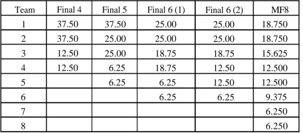
TABLE 7.1. Premiership chances for MF8 and previous final systems

With each new system, the chances of teams 1 and 2 have been steadily eroded until they are now exactly half of that under the final four. Team 3's chances doubled with the introduction of the final five, but have since been eroded although they are still greater under the final eight than under the final four. Thus even though the number of finalists has doubled, team 3's chances have increased. Team 4's chances have enjoyed a roller coaster ride, but have settled on exactly the same probability as for the final four. Team 6's chances have increased as have teams 7 and 8. In economic terms, we have seen a great redistribution of probability from the rich top order to the poor lower order, with the

Team 1 2 3 4 5 6 7 8 Final 4 37.50 37.50 12.50 12.50 Final 5 37.50 25.00 25.00 6.25 6.25 Final 6 (1) 25.00 25.00 18.75 18.75 6.25 6.25 Final 6 (2) 25.00 25.00 18.75 12.50 12.50 6.25 MF8 18.750 18.750 15.625 12.500 12.500 9.375 6.250 6.250

middle class largely unaffected. Teams 7 and 8 now have as much chance of winning as 4 and 5 had under the final five system. However one should note that this is only 1 in 16, actually less than they had at the start of the season (1 in 15 if there are 15 equal teams). Clearly the AFL have not been interested in maximising the chance of the highest-ranked team winning, but they have produced a system in which a team's chances increase steadily with their ranking.

One consequence of the diminution of the top team's chances is that the league should consider recognising the team who finishes at the top of the ladder before the finals, perhaps with a minor premiership cup, since their chances of turning that position into a premiership is now much smaller than under earlier final systems.

7.4. Importance of matches

Football supporters know the grand final is the most important match of the year. It would be desirable if finals matches built up in importance, but how can we quantify this notion of importance? Morris (1977) defines the importance of a point in tennis as the difference in the probability of winning the match if a player wins the point and the probability of winning the match if a player loses the point. Thus the grand final is the most important match at loo%, with the preliminary final at 50%. The calculations are shown below.

Grand final 100%-0%

Preliminary final 50% -0%

Semi-final 25% -0%

Qualifying final between 1 &8 (or 2&7)

For team 1,2 25% - 12.5%

For team 8,7 12.5%

-

0%

Qualifying final between 4825 (or 3&6)

Depends if 1 and 2 lose 25%- 0% or if 1 and 2 win 12.5%-12.5% or if 1 and 2 win and team 1 plays interstate

= 25% = 0% negative?

In general the matches are in order of increasing importance. However as we have said, the qualifying finals also have importance to other teams. The definition of importance needs extending to take this into account, perhaps to the total expected absolute change in probability of all the teams. When this is done the importance of the qualifying finals

increases. Note that a win by the lower-ranked teams in the matches lv8,2v7 and 3v6 is good for the winner of the other qualifying finals and bad for the loser - so it makes those matches much more important. For this reason, the importance of the qualifying finals 3v6 and 4v5 is more difficult to calculate, as it depends on the results of other finals.

One special case is worth discussing. In order to maximise crowd attendance and television coverage, the finals are played at different times over a weekend. Thus it is possible the league could schedule the match between 4 & 5 (or 3 & 6) after the other qualifying matches. If the other qualifying matches have both gone to the higher-ranking team, then these matches would be of zero importance, since the winner cannot make the bye and the loser cannot be eliminated. The only factor hinging on the match is which half of the draw the teams go into. We could even have the situation where one or even both teams are trying to lose, to avoid the half of the draw containing specific teams. For example, two interstate teams may already be in the half of the draw into which the winner will go. It is highly likely matches against these interstate clubs would be scheduled on their home grounds, a large disadvantage to any Melbourne team drawn to play them. A 4v5 qualifying final between two Melbourne clubs could see the winning team having to play two finals interstate to make the grand final

-

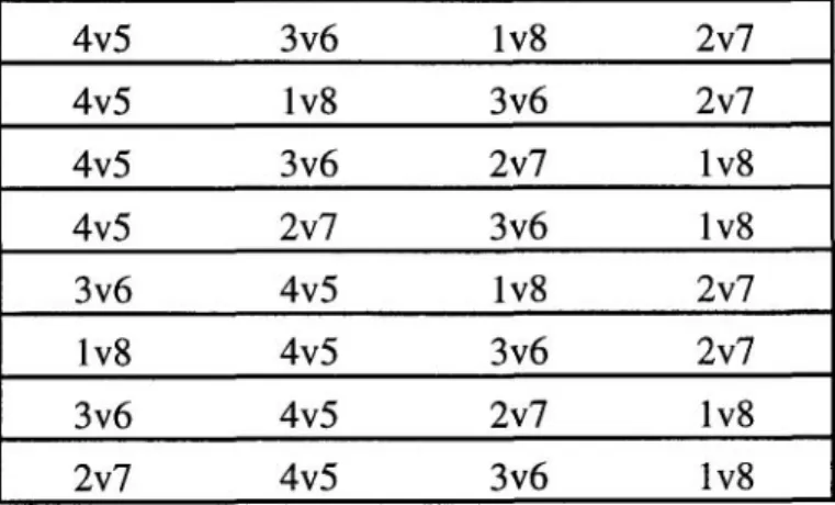
with the loser having the easier draw of two games in Melbourne. To avoid this situation the qualifying finals need to be played in a certain order. The match 4v5 must be played in the first two finals, and the match 3v6 in the first three finals. The problem is equivalent to ordering the digits 1, 2, 3, and 4 so that no digit is preceded by two or more lower numbers. The possible orders are shown in Table 7.2. In 1994, the AFL chose the second last shown. Note that this does not stop a final being 'dead' in retrospect. In 1994 the 4v5 clash between Geelong and Footscray, won by the final kick of the match, was in fact in this category. Neither team was eliminated, so in fact the result did not matter.

7.5. Development of program using a word processor

Schwertman & Howard (1989, 1990) look at a probability model for the AFL Finals series as it was played up to 1990 - a series of six games between the top five teams. They list the four paths that result in the fourth team winning the grand final, and the 16 paths that result in the second team winning. For the top team they say "Direct computation of the probability that team A wins the grand final is quite involved, with many different paths" and suggest indirect methods. The MF8 is a series of nine matches with the extra complication that the position of a winning team now depends not just on their match but on the results of other matches. Clarke (1993a) gives a method for determining all possible finishing orders for the final six, and that is extended here.

For the MF8, we wish to calculate not only the chance of each team winning the grand final, but also some other probabilities of interest such as the chance of pairs of teams making the grand final and the chance of each team finishing in any position. All the probabilities would follow from the chance of all possible finishing orders. So the problem was: "Given the original order before the finals, what is the probability of any final finishing order?" Although in studying the fairness of the finals system it is of interest to assume all teams are of equal ability, for the computer tip we had different probabilities for any team beating any other. Furthermore, because the computer tipping program takes grounds into account, the probabilities changed from week to week depending on the grounds at which the matches were scheduled.

Suppose we designate each team by their finishing position at the end of the home and away matches. Using the actual results from 1994, we have a sequence of matches as follows, where positions and teams are: I West Coast, 2 Carlton, 3 North Melbourne, 4 Geelong, 5 Footscray, 6 Hawthorn, 7 Melbourne, 8 Collingwood.

Week 1 Week 2 Week 3 Week 4

1-8 (1 wins) 4-2 (4 wins) 3-4 (4 wins) 1-4 (1 wins) 2-7 (7 wins) 5-7 (7 wins) 1-7 (1 wins)

3-6 (3 wins) 4-5 (4 Wins)

The final finishing order produced by this particular sequence of results and its associated probability is:

where pk(i j) is the probability of team i beating team j in week k. There is no obvious pattern between the final order and the probabilities that produce that order. It would be tedious in the extreme to work out all possible 29 = 512 sequences and their probabilities. The fact that positions of teams depend not just on the results of their matches but on the results of others, further complicates matters. However a word processor comes to our aid. A modern word processor allows the copying and movement of columns of text as well as rows of contiguous text. Using this facility, the 5 12 lines of code that formed the crux of the program were written in about 1 hour.

The method involves keeping on the left side the 'current' order and on the right side the probabilities of that order arising. Each match result has a certain probability and produces an associated change in the order. Before the final series the order is

1,2,3,4,5,6,7,8 so we have:

Order Probability

Consider the match between 4 and 5 This can have two results, so we copy the whole row. Now if 4 beats 5 the order stays the same, so we leave the first row alone, but if 5 beats 4, 5 moves to 4th and 4 moves to 5th, so we do this to the second row. This gives us:

We now want on the right side the probabilities of these results

-

i.e. p1(4,5) in the first row and p1(5,4) in the second. But these are just the numbers in the middle two columns of the left side. Thus we can use the column copy and insert facility on the word processor to copy them across. This gives:

We have added the pk()s for ease of reading, but in practice, these were all inserted at the end of the process. We repeat the procedure for the remaining matches. Each match iteration results in a doubling of the number of rows with a duplication of the whole table, the movement of columns on the left side, and the addition of another set of pks by copying parts of columns from the left to the right of the table. With column copy and insert and global replace it was about an hour's work to produce 512 lines similar to (7.1) and convert to code. In this case SAS was used, but other packages such as Excel could be utilised. A SAS data set with two variables, order and probability was created, and the above lines of code produced 5 12 observations. Programming and SAS procedures could then be used to calculate any required probabilities.

In the author's original problem, the normal weekly computer tipping program was used to provide probabilities for each team beating any other, and the above program was used both before and during the final series to predict estimated probabilities of teams winning the flag or finishing the year in different positions. These predictions were included with the usual ones of winners and margins. The program thus served its original purpose.

However the program can also be used to investigate the degree to which the MF8 satisfies the criteria for fairness discussed earlier.

7.6. How fair is the MF8?

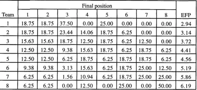
Schwertman & Howard (1990) suggest several suitable models to investigate the fairness of finals systems. Here we assume that all teams are equal. The qualifying finals in 1994 showed this is not an unreasonable model, with team 8 losing to team 1 by two points, team 6 and team 3 drawn at full time, team 4 beating team 5 with the last kick of the match and team 7 beating team 2 comfortably. Tables 7.3, 7.4, 7.5 and 7.6 give some output from the program that demonstrates the MF8 performs well on the fairness criteria. The chance of winning and the expected final position (EFP) are in order of original ranking. In fact the chance of finishing in position j or higher is in monotonic order of original ranking for every j. The chance of team i finishing above team j is generally in increasing order of j for every i, with a couple of exceptions for teams widely separated in the rankings.

TABLE 7.3. Percentage chance of teams finishing in any position, and expected final position (EFP) - Equal probability model

TABLE 7.4. Percentage chance of teams finishing in any position or higher - Equal probability model

TABLE 7.5. Percentage chance of team i (row) finishing above team j (column) - Equal probability model

The chance of grand finals between the teams in various positions is shown in Table 7.6, and is roughly in accord with the sum of the teams' rankings. A grand final between 1 &

2 is the most likely result, although it only has about a 1 in 8 chance of occurring, compared with 1 in 2 under the old final four system. The chance of a grand final between 2 & 3 is relatively low because of the high probability they will end up in the same half of the draw. Note also that two grand finals are impossible

-

between 2 & 8 and 1 & 7. However this did not stop the National Sportsbook from offering odds of 100-1 on a Collingwood-Carlton grand final, and 50-1 on a West Coast-Melbourne grand final in the week preceding the qualifying finals in 1994.

TABLE 7.6. Percentage chance of pairs of teams playing in grand final - Equal probability model

7.7. Comparison of bookmakers' and computer's odds

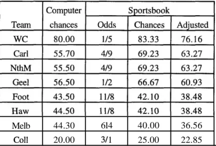
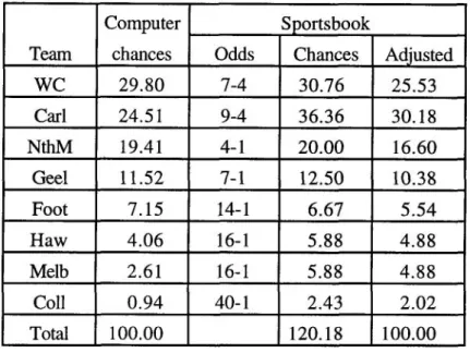
It is interesting to see the extent to which bookmakers' odds reflect the intricacies of the finals draw. The head to head odds for the first match along with the premiership team and quinella (the two teams that play in the grand final) odds offered by the National Sportsbook as published in The Melbourne Herald Sun, September 10, 1994 are given in Tables 7.7-7.9. Odds of a h are converted to percentage chances as 100*b/(b+a). As these usually sum to more than 100 due to the bookmaker's percentage, adjusted chances which are proportional but sum to 100 are shown. For comparison the head to head chances as estimated by the computer tipping program and the consequent premiership and quinella chances are also given.

It is clear the Sportsbook odds often do not reflect the intricacies of the MF8. Although Sportsbook give North Melbourne a greater chance of winning the first match (63% as against 56% by the computer), they are given less chance (16% as against 19%) of winning the premiership. This apparently underestimates their chance of gaining the double chance. Geelong is treated in the same way. Although Melbourne is given less chance of winning the first match than Hawthorn, they have the same chance of winning the flag, completely discounting Hawthorn's possible bye or double chance.

TABLE 7.7. Comparative chances of winning first match

Melb Coll 44.30 20.00 36.56 22.85 614 31 1 40.00 25.00

TABLE 7.8. Comparative premiership chances

TABLE 7.9. Computer chances and Sportsbook odds on quinellas

The quinellas also show inconsistencies. An obvious case is the Carlton-Collingwood and West Coast-Melbourne quinellas. These are both impossible, yet are not only given odds but are shown at shorter odds than many possible quinellas. The Carlton-North quinella is also misquoted. Tables 7.6 and 7.9 show this to be quite unlikely, due to the high probability of team 3 and 4 ending up in the same half. A more detailed analysis shows that team 2 and 3 will only end up in opposite halves if in week 1, team 1 wins and 2 and 3 both lose, or team 1 loses and 2 and 3 both win. Using the adjusted Sportsbook odds on this occurring from Table 7.7 we obtain a probability after week 1 of only 0.2 that a Carlton-North grand final will still be possible. Either two or four matches will still have to fall the correct way for the grand final to eventuate. The odds of

10-1 are thus extremely poor and overestimate the chance of this particular grand final. In a similar way, the extra difficulty of obtaining a West Coast-Hawthorn quinella over a West Coast-Carlton quinella that is shown in both Table 7.6 and Table 7.9 is not reflected in the Sportsbook odds.

7.8. Home advantage

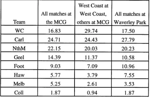
There are two large capacity Melbourne grounds on which finals have been traditionally played, the MCG and Waverley Park. However, finals in the first three weeks involving interstate teams are likely to be played at their home venue. Since the MCG and Waverley are shared as home grounds by several Melbourne teams, there is a considerable home advantage (HA) element in the finals. Stefani & Clarke (1991, 1992) have calculated home ground advantages in home and away matches in AFL football. The computer program developed here can also be used to quantify HA in the finals. By altering the venues for matches in a particular week, the effect on a team's premiership chances can be evaluated. Table 7.10 shows the final program's estimated chances of winning the premiership using the weekly computer tipping program's probabilities of winning each match under various venue assumptions. The first column shows the program's calculated premiership chances if all matches are played at the MCG, the second with matches involving West Coast moved to West Coast the first three weeks, and the third with all matches in the first three weeks played at Waverley. In general this shows a multiplier effect if teams play several matches at home. Thus a team that wins 10% more matches at home may win 30% more premierships if all matches are played at home.

The effects are quite dramatic. West Coast's chances almost double by having the preliminary matches at home, although their average chance of winning at the West coast is 'only' 47% higher than at the MCG. By moving all preliminary matches to Waverley, Hawthorn's chance increases by 31% although their average chance of winning at Waverley is only 11% higher than the MCG. Similarly Melbourne's chance would reduce to 67% although their average chance of winning at Waverley is 89% of their chance at the MCG. While one could argue about the magnitude of individual home effect, the general point is that, because of the knockout nature of the finals series, individual home ground effects are magnified when considering the chances of winning the premiership.

TABLE 7.10. Premiership percentage chances if matches in the first three weeks at different grounds

7.9. Conclusion

In football, subjective judgements are often used to rate team chances of winning the premiership. These often tend to reflect the relative strengths of the teams, and ignore the current ladder position. With the complicated structure now in place for the finals series, a mathematical analysis using a simple model can shed light on the chance of teams winning or finishing in any position, given their original or current ranking in the final series. One aspect of mathematics is recognition of patterns. In this case, there was no obvious pattern between the final order and the probabilities that produced that order. However, there was a pattern in the way these orders and probabilities were built up when individual matches were considered. The functions of a word processor could be used to exploit this pattern to write the required equations and subsequent computer code. The code generated was flexible enough to handle many different models.

It is important to investigate how a sport's draw operates, rather than complaining when a specific unforseen case arises. Teams cannot be blamed when they 'exploit' weaknesses in the rules of a competition that organisers have allowed to creep in. There are many criteria that a final series should satisfy. For many competitions the relative chances of teams finishing in any position, not just first, should be considered. The MF8 passes most of the tests given here. The higher a team finishes at the end of the home and away matches, the greater their chances of being the premier team, the greater their chances of finishing in any position or higher, the higher their final expected position, and the

greater their chances of finishing above lower teams. However two major flaws exist. The first is that a team's chances depend so much on matches in which it does not participate, which results in a lack of consistency from year to year. There seems little, other than a new system, that the AFL could do to redress this. The other major weakness that may need to be addressed is the possible lack of importance of the qualifying finals between 4 & 5 and 3 & 6. It seems a great pity that a final would degenerate into a 'dead' match, or worse still a farce where both teams were trying to lose. The AFL must always schedule these matches early so the chance of the winner making the preliminary final direct or to avoid elimination exists to give the teams incentive. Of course matches will still often be dead in retrospect, as occurred in 1994. Because of the greatly reduced chances of a team winning the flag from top position, the league should consider recognising the leader after the home and away matches by a minor premier cup.

It is also clear that a computer program, such as detailed here, could be useful in assisting with framing the odds for premierships and quinellas under a system as complicated as the MF8.

7.10. Commentary. Increasing influence of HA in finals

Since this paper was written the home ground advantage in finals has continued to have a strong influence. As interstate teams grow in number and strength, more finals include a home ground factor. In 1996, due to the presence of Essendon and North Melbourne (both if which have the MCG as home ground), and three interstate sides, each of the nine finals included exactly one team playing on their home ground. All nine finals were won by the team with the HA.

7.11. Commentary. Quantifying the effect of AFL decisions on the home and away draw

All sports are affected by the overall rules of the competition. The previous paper quantified the effects of the various final systems. The models discussed in the thesis can also be used to quantify AFL decisions that affect the home and away draw. The League along with individual clubs makes many decisions affecting the running of the competition. These are often based on financial aspects such as to maximise crowds or television exposure, but they also affect teams' chances of success in the competition. They range from relatively minor changes such as moving the venue of a single match or

moving the home ground of a club for an entire season, through to decisions having major ramifications such as organising an unbalanced draw. What effect do these have on a team's chances? In the past these have not been quantified. The remainder of this chapter shows how some of these aspects can be investigated.

7.11.1. Change of venue

By using the estimated ground effects developed by the computer tipping program, the effects of changing venues on the chance of teams winning can be evaluated. The AFL often move particular matches. This may be to allow for anticipated large crowds, or the poor state of the surface of a particular ground or for other reasons. Sometimes it is done with the approval of the affected clubs, but often against their wishes. Clubs will often cite the loss of their HA as a reason against the move, but never is this quantified. It now can be.

For example, suppose it is mooted that the 1996 round 14 Footscray-Melbourne match be moved from the MCG to Footscray. In fact several of Melbourne's home matches have been moved, to leave the MCG free for matches expected to draw large crowds. As at round 1 1, 1996, the computer rated Melbourne at 52.2 and Footscray 56.2. However the ground effect for Melbourne at the MCG was 1.8, and for Footscray -6.8. Thus the HA to Melbourne at the MCG was 1.8

+

6.8. At the Whitten oval it was 9.9

+

0.4 to Footscray. Thus, using equation 4.3, at the MCG the expected result is a 3.6 point win to Melbourne, whereas at Footscray it is 14.3 win to Footscray. In terms of percentage chances, this changes Melbourne from a 53% chance to a 38% chance. Thus the change of venue resulted in a decrease of 15% in Melbourne's chances of winning. If this was repeated over 11 home matches it would be almost two extra losses by the club.

A similar analysis can be performed for a team that changes its home ground permanently. In 1993 St Kilda moved from Moorabbin where they enjoyed one of the highest HAS of 12.5 (compared with an average of -0.5 for the other teams) to Waverley Park where they had a negative ground effect (-4.8 at the end of 1995, compared with the average for the other teams of 0). By the methods of the previous paragraph the change cost them on average over 17 points each home match, or a decrease in percentage chance of winning of about 15%. This results in an expected decrease in the number of wins in their 11 home matches of 1.7. While this may not seem a lot, in 1993, although finishing 12th, they were only two wins behind Adelaide who finished 5th. In 1995, an extra 1.5 wins would have taken them from 14th to at least 9th on the final ladder. It is clear the move to

Waverley has been costly to St. Kilda in terms of its on-field success.

7.11.2 Fairness of draw

-

average strength of opponents

A major drawback of the League competition is that the draw is not balanced. It is unbalanced with respect to strength of opposition (each team plays a different set of opponents twice) and with respect to grounds (teams play a different number of matches on their home grounds). While the general public recognise this is inequitable, again it has never been quantified in a proper manner. At the very most a football writer may tabulate the number of times each team plays a weak team, or a finalist from the previous season, but never is it done at the end of a season when the true strengths of the teams is better able to be estimated. This unfairness will not necessarily even out over the years. For example at one time the draw was made on the basis that the top teams in one year played each other twice the following year. Thus there was an ongoing bias in the draw.

It is relatively simple in principle to quantify the unfairness of the draw after the season. An analysis such as performed in section 2.14 gives team rating and HAS. Unlike other measures such as final ladder positions or percentage, these are independent of the toughness of the draw. Summing the ratings of the opponents of each team gives a measure of the difficulty of the draw for that team. This is equivalent to the approach of (Leake, 1976) who suggested the average rating of opponents as a measure of schedule difficulty. The home ground advantage of opponents could also be included as this contributes to the draw difficulty. However there are problems with this approach. Since the good teams do not play themselves, they will appear to have an easier draw than the others. Thus even in a balanced competition this method would give a measure of unbalance. For this reason we need to subtract the average strength of the opponents. Thus we are measuring the excess strength of the actual opponents over the average strength of all possible opposition. This is equivalent to adding a proportion of a team's own rating to account for the above bias.

If the measure of team ability in an N team competition is ui, i = 1 to N, where Cui = 0,

then opponent j will exceed the average strength of all possible opponents of team i by

Z U i

j t i - _{u. --} -Ui _=u,+- Ui

Summing this for all opponents is a measure of the total strength of opposition to team i. While we could use the us derived earlier, or better still ui

+

0.5 hi, there are advantages in using a measure that the general football follower would understand. For this reason, percentage, which Figure 2.4 showed was highly correlated with ui

+

0.5 hi, may be a good choice.

A well understood measure of a teams ability is final ladder position. This incorporates both team ability and some measure of HA. Unfortunately it also includes a component due to the factor we are measuring - draw difficulty, but we bear with this in the interests of having a simple measure. While it would be more accurate to use (say) the regression estimates of a team's ability rather than ladder ranking, the latter has the advantage of being understood by the average administrator and supporter. Table 7.11 was obtained using the ladder ranking at the end of the year. Because a low number indicates a high ranking and strong opposition, a negative total indicates the draw was more difficult than average, a positive number easier than average. Note that during the years 80 to 86 all teams had a balanced draw. In other years, the difference between highest and lowest is generally about 35. This is clearly a significant amount, particularly for two teams in a similar position on the ladder, where the difference cannot be attributed to the different rankings of the two teams. For example in 1988, Geelong, one position on the ladder ahead of Richmond, had a more difficult draw by 36 ranking points. That is the equivalent of playing the top three teams instead of the bottom three teams. In the same year West Coast finished one spot above Melbourne with the same number of wins. However Melbourne's draw was 29 ranking points harder than West Coast. A similar draw could have given Melbourne three extra wins and put them second on the ladder. (They actually did win their way through to the grand final). In 1995, the two teams with the hardest draw, Melbourne and Collingwood both missed the final eight by one game, even though they had better percentages than Footscray who finished seventh and Brisbane who finished eighth. Again the difference in their draw difficulty could easily account for the difference. It is clear that the degree of imbalance that exists in the draw is enough to have a significant effect on the final ladder outcomes. Individual clubs should also look at their draw difficulty in assessing the measure of success they have achieved through the year.

Clearly the draw difficulty does not even out through the years. Richmond and Sydney appear to have had a long run of good draws, while Carlton has had a long run of more difficult draws. Many AFL clubs have criticised the level of financial support given to Sydney. They have also, it appears, received support from the schedule.

7.11.3 Fairness of home and away draw

-

as assessed by the computer prediction

In this section we demonstrate how the computer prediction program can be used to obtain another estimate of the effect of the draw on the success of clubs. This gives a measure of the effect in ladder positions. Particular goals for clubs would be to make the finals, make the grand final and win the premiership. Any sporting competition is designed to produce a winner, and the rules should ensure the expected final positions reflect the abilities of the participants. The ladder prediction model described in section 4.2.1 provides a perfect tool to investigate this. Given the ratings of each team and the draw it provides the expected finishing position of all teams. This can be compared with the ratings. This is demonstrated with a detailed look at 1995.

The computer prediction program was used to predict the 1995 results using the initial ratings derived from the previous year. The ratings of each team at the end of each round were recorded and plotted. This showed that the rating of a team is certainly not constant over a year, that teams have periods of good and poor form. (To ensure this was not just an apparent affect because the initial rating was in error, the average rating was calculated for each team and the program run again with these ratings as the initial ratings. Most teams still showed the same general pattern - as the rating is in effect a smoothed average, the initial ratings only affect the first few week's ratings). Figures 7. l a and 7. l b show the week by week ratings of a couple of teams along with their average rating. Clearly Collingwood has played the last half of the of the season much better than the first half, while Brisbane has made a tremendous improvement from about Round 15 onwards. Many of these graphs are interesting in their own right, and could be used to investigate the effects of changes, such as injury to star players, changes of coach etc. For example, the Brisbane coach announced his decision to retire at the end of the year about Round 15. In the round 15 match, Brisbane overcame a 45 point deficit at three quarter time to beat Hawthorn by 7 points. The victory was put down to the visiting team wilting in the heat, but the effects were obviously seen for the remainder of the year. Brisbane's rating shows a steady rise from that point and they made the finals for the first time. Hawthorn's ratings decreased just as steadily, and they finished second last, missing the finals for the first time in since 198 1. While such a spectacular change in fortune can be picked up by other means, graphs such as these can be used to study a team's form. Their advantage is they have allowed for ability of opposition and HA. Currently winning and losing streaks are often used, but these are affected to a great degree by quality of opposition.

Figure 7. la. Weekly ratings of Brisbane during 1995 75.00 70.00- 65.00- .g 60.00- rn 55.00- 50.00- 45.00 65.00 1 1 1 1 1 1 1 1 1 1 1 1 1 1 1 1 1 1 1 1 1 1 0 1 2 3 4 5 6 7 8 9 1 0 1 2 1 4 1 6 1 8 2 0 ... 1 1 1 3 1 5 1 7 1 9 2 1 Round

. . . ..

- 1

.

1 1 1 1 1 1 1 1 1 1 1 1 1 1 1 1 1 1 1 1 1 1

Figure 7.lb. Weekly ratings of Collingwood during 1995

0 1 2 3 4 5 6 7 8 9 1 0 1 2 1 4 1 6 1 8 2 0

...

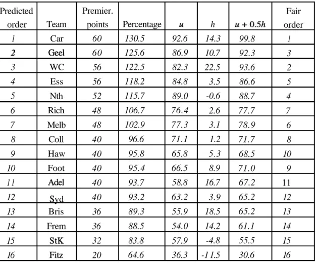
1 1 1 3 1 5 1 7 1 9 2 1 Round

We cannot expect a draw to be balanced for this change of form for different teams. Always some teams will be lucky and play opposition when they are down on form or missing star players. However it should be balanced for average ability. The average ratings for the year were used as initial ratings for the computer predictions. (That actually increased the predicted number of winners for the home and away matches for the year from 127 to 134, and reduced the margin of error from 32.6 points to 31.2 points. This gives a measure of the value of the unknown information, average form level, at the start of the year.) The final ladder predictions assume current form and HAS for the remainder of the year, so the computer predictions before round 1 of the final ladder can be used to estimate the expected finishing positions of each team. In a perfectly balanced competition balanced for quality of opposition and HA, the expected final ladder would be roughly in the same order as u+ 0.5h. Variations from this reflect unfairness in the draw. The expected ladder produced by the program, along with the team ratings and HAS are given in Table 7.12.

Note the predicted order is in good agreement with the fair order. However teams that have done better than fair are Geelong, Essendon, Richmond and Hawthorn. Those that have done worse are West Coast, North Melbourne, Melbourne and Footscray.

Some of these results are consistent with the previous results on draw difficulty. The two teams with the easiest draws both do better than expected and Melbourne with a hard draw does worse. Again, there are probably competing effects here. Some can be attributed to their poor ground effect at the MCG. The major difference is that the previous was based on actual ladder position whereas this method used average rating for the year.

TABLE 7.12. Expected final ladder for 1995, with team ratings and HAS shown

7.11.4. Using simulation to measure the efficiency of the draw Of course the actual ladder positions will be due to some extent on random variation. We might wish to investigate the extent to which the final ladder position is affected by random variation. A season of football has a large random element, and most supporters recognise that luck plays some part in the success of their club. Also club success is not a linear function of ladder position. For example, obviously two seconds would not be equivalent to a first and third. For both these reasons it is appropriate to look at the probabilities of teams achieving certain goals. In racquet sports, for instance, this has resulted in the concept of efficiency of scoring systems, where the length of matches is traded off against the probability of the better player winning.

Predicted order 1 2 3 4 5 6 7 8 9 10 1 1 12 13 14 15 16

While it is outside the scope of this thesis to investigate alternatives, we do want to give an idea of the effects of random variation on the final ladder. The simulation discussed in section 4.2.1 will give us an indication of its extent. Table 7.13 is the result of

Premier. points 60 60 5 6 56 52 48 48 40 40 40 40 40 3 6 3 6 32 20 Team Car Gee1 WC Ess Nth Rich Melb Coll Haw Foot Adel S y d Bris Frem StK Fitz Percentage 130.5 125.6 122.5 118.2 115.7 106.7 102.9 96.6 95.8 95.4 93.7 93.2 89.3 88.5 83.8 64.6 u 92.6 86.9 82.3 84.8 89.0 76.4 77.3 71.1 65.8 66.5 58.8 63.2 55.9 54.0 57.9 36.3 h 14.3 10.7 22.5 3.5 -0.6 2.6 3.1 1.2 5.3 8.9 16.7 3.9 18.5 14.2 -4.8 -1 1.5 u + 0 . 5 h 99.8 92.3 93.6 86.6 88.7 77.7 78.9 71.7 68.5 71.0 67.2 65.2 65.2 61.1 55.5 30.6 Fair order 1 3 2 5 4 7 6 8 10 9 1 1 12 13 14 15 16

simulating the 1995 season 1000 times using the average rating for the teams as initial ratings. The table shows the number of seasons the team finished in the given position. While the most likely position was generally close to the ranking based on u

+

0.5h given

in Table 7.12, the probability of this was often quite low. The table shows the huge variation possible in a season of football and demonstrates the dangers in putting too much emphasis on the final ladder position as a measure of the team's performance. It is possible for almost any team to finish anywhere from last to first due to the random effects. The range within which a team was an 80% chance to fall within was about four positions for the very best and worst teams, up to about 10 positions for some of the middle teams. This dependence on chance can be demonstrated by looking at individual matches. In round 9, Adelaide beat Hawthorn 9.06 to 7.16 by two points. Had just one of Hawthorn's 16 behinds been a goal, Hawthorn's final ladder position would have been three places higher and Adelaide 4 places lower. In contrast, the ui and hi for those teams as developed in section 2.14 would have hardly altered at all. For this reason, measures as suggested in this thesis are a more accurate reflection of a team's performance through the season.

TABLE 7.13. Chances in 1000 of ending in any position after home and away matches Footscray Geelong Hawthorn Melbourne NthMelbourne Richmond Sydney St. Kilda Brisbane West Coast Fremantle 3 236 2 18 103 26 4 1 1 184 1 5 185 13 38 114 53 6 2 4 189 3 21 170 27 53 124 73 15 4 10 156 6 39 121 44 68 114 90 22 7 16 139 9 36 93 50 82 125 117 36 12 24 91 23 66 59 70 106 104 114 59 18 36 77 33 93 52 78 98 88 95 59 21 48 63 39 31 110 98 66 110 85 30 56 32 62 8 6 1 0 2 22 78 95 41 79 99 63 68 25 59 11 107 91 43 91 87 62 100 18 93 9 9 1 1 3 1 0 7 7 91 66 33 37 114 88 102 14 94 5 103 59 21 46 110 102 102 5 131 95 6 76 59 9 30 104 116 147 5 129 71 2 76 49 9 24 104 152 126 1 137 53 0 61 18 5 14 76 241 137 1 136 11 0 14 2 1 1 20 81 23 0 45