Directed Models For Statistical Relational Learning

LEARNING

by

Hassan Khosravi

M.Sc., AmirKabir University of Technology, 2007 B.Sc, Shahid Bahonar University, 2005 a Thesis submitted in partial fulfillment

of the requirements for the degree of

Doctor of Philosophy in the

School of Computing Science Faculty of Applied Sciences

c

Hassan Khosravi 2012 SIMON FRASER UNIVERSITY

Fall 2012

All rights reserved.

However, in accordance with theCopyright Act of Canada, this work may be reproduced without authorization under the conditions for “Fair Dealing.” Therefore, limited reproduction of this work for the purposes of private study,

research, criticism, review and news reporting is likely to be in accordance with the law, particularly if cited appropriately.

Name: Hassan Khosravi

Degree: Doctor of Philosophy

Title of Thesis: Directed Models for Statistical Relational Learning

Examining Committee: Dr. Anoop Sarkar,Associate Professor, Computer Science Chair

Dr. Oliver Schulte, Associate Professor, Computing Science

Senior Supervisor

Dr. Martin Ester, Professor, Computing Science Supervisor

Dr. Lise Getoor, Associate Professor, Computer Sci-ence

University of Maryland External Examiner

Dr. James Delgrande Professor, Computing Science Internal Examiner

Date Approved:

ii

Statistical Relational Learning is a new branch of machine learning that aims to model a joint distribution over relational data. Relational data consists of different types of objects where each object is characterized with a different set of attributes. The structure of re-lational data presents an opportunity for objects to carry additional information via their links and enables the model to show correlations among objects and their relationships. This dissertation focuses on learning graphical models for such data. Learning graphical models for relational data is much more challenging than learning graphical models for proposi-tional data. One of the challenges of learning graphical models for relaproposi-tional data is that relational data, unlike propositional data, is non independent and identically distributed and cannot be viewed in a single table. Relational data can be modeled using a graph, where objects are the nodes and relationships between the objects are the edges. In this graph, there may be multiple edges between two nodes because objects may have different types of relationships with each other. The existence of multiple paths of different length among objects makes the learning procedure much harder than learning from a single ta-ble. We use a lattice search approach with lifted learning to deal with the multiple path problem. We focus on learning the structure of Markov Logic Networks, which are a first order extension of Markov Random Fields. Markov Logic Networks are a prominent undi-rected statical relational model that have achieved impressive performance on a variety of statistical relational learning tasks. Our approach combines the scalability and efficiency of learning in directed relational models, and the inference power and theoretical foundations of undirected relational models. We utilize an extension of Bayesian networks based on first order logic for learning class-level or first-order dependencies, which model the general database statistics over attributes of linked objects and their links. We then convert this model to a Markov Logic Network using the standard moralization procedure. Experimental

Doing a Ph.D. is a long journey and is only possible with the supervision of my committee members and moral and physical support of family, my partner, and friends.

First of all I would like to express my deepest gratitude to my senior supervisor, Dr. Oliver Schulte, for his excellent guidance, kindness, patience throughout my Ph.D. He has helped me develop many skilled during our collaboration. I would never have been able to finish my dissertation without his guidance and support. I would also like to thank my supervisor, Professor Martin Ester, for his guidance, support and willingness to help. I am grateful to Dr. Lise Getoor, Dr. Jim Delgrande, and Dr. Anoop Sarkar for willing to participate in my final defense as external examiner, internal examiner, and chair.

I would like to thank my wife Rozita for all her love and support. All of the nights we spend together studying, and her encouragements was in the end what made this dissertation possible. I would also like to thank my parents, two sisters Sara and Rana, and brother in law Reza. They were always very supportive and encouraged me with their best wishes.

Special thanks go to all of the collaborators, other students, that I had the honor of work-ing with durwork-ing my Ph.D. Bahareh Bina, Ali Bozorgkhan, Tong Man (Mike), Xianoyouan Xu(Vivian), Jianfeng Hu, Tianxiang Gao, and Yuke Zhu have all been super collaborators. Finally, I would like to thank all the friends that have been there for me during my stay at Simon Fraser University. My roommates, Mohammad, Ehsan, Alireza, and Bamdad for putting up with me, and of all other friends Majid, Maryam, Nima, Bardia, Arina, Maryam, Esmaeil, Kouhyar, Hossein, Shahab, Hamed, Kamyar, and Amir for the coffees, swimming, tennis, racketball, shelem and xbox time that we spend together.

Approval ii Abstract iii Dedication v Quotation vi Acknowledgments vii Contents viii

List of Tables xii

List of Figures xiv

1 Introduction 1

1.1 Approach . . . 2

1.2 Contributions . . . 4

1.3 Limitations . . . 4

2 Background and Literature Review 6 2.1 Background and Notation . . . 6

2.1.1 Probability Distribution . . . 7

2.1.2 Logic . . . 7

2.1.3 Machine Learning . . . 8

2.1.4 Bayesian Networks . . . 9

2.2 Probabilistic Relational Models(PRMs) . . . 18

2.2.1 Representation in PRMs . . . 18

2.2.2 Inference in PRMS . . . 19

2.2.3 Learning In PRMs . . . 20

2.3 Markov Logic Networks(MLN) . . . 23

2.3.1 Representation in MLNs . . . 23

2.3.2 Inference in MLN . . . 26

2.3.3 Learning in MLN . . . 27

2.4 Relational Dependency Networks(RDNs) . . . 29

2.4.1 Learning in RDNs . . . 31

2.4.2 Inference in RDNs . . . 32

2.5 Baysian Logic Programs (BLPs) . . . 33

2.5.1 Representation and Learning in BLPs . . . 33

2.5.2 Learning in BLPs . . . 34

2.5.3 Inference in BLPs . . . 36

2.6 Comparison with previous work . . . 36

3 Learning Graphical Models via Lattice Search 40 3.1 Introduction . . . 40

3.1.1 Approach . . . 41

3.2 Related Work . . . 42

3.2.1 Lattice Search Methods . . . 42

3.2.2 MLN structure learning methods . . . 43

3.3 Lattice Search for Attribute Dependencies . . . 45

3.3.1 Overview . . . 45

3.3.2 The Multinet Lattice . . . 45

3.3.3 Model Conversion . . . 49

3.4 The Learn-And-Join Algorithm . . . 49

3.4.1 Constraints Used in the Learn-And-Join Algorithm . . . 50

3.4.2 Example of Learn-and-join Algorithm . . . 53

3.4.3 Discussion: Lattice Constraints . . . 54

3.5.1 Datasets . . . 58

3.5.2 Graph Structures Learned by the Learn-and-Join algorithm . . . 60

3.6 Moralization vs. Other Structure Learning Methods: Basic Comparisons . . . 61

3.6.1 Comparison Systems and Performance Metrics . . . 61

3.6.2 Runtime Comparison . . . 62

3.6.3 Predictive Accuracy and Data Fit . . . 63

3.6.4 UW-CSE Dataset . . . 66

3.6.5 Comparison with Inductive Logic Programming on Mutagenesis . . . . 67

3.6.6 Lesion Studies-Lattice Constraints . . . 68

4 Graphical Models with Recursive Dependencies 72 4.1 Introduction . . . 73

4.2 Example . . . 74

4.3 Related Work . . . 75

4.4 Directed Models and Recursive Dependencies . . . 76

4.4.1 Inference in Directed Models with Recursive Dependencies . . . 77

4.4.2 Model Selection in Directed Models with Recursive Dependencies . . . 78

4.5 Redundancy in Directed Models with Recursive Dependencies . . . 79

4.5.1 Stratification and Recursive Dependencies . . . 80

4.5.2 Stratification and the Main Functor Node Format . . . 82

4.5.3 Discussion. . . 84

4.6 The Learn-and-Join Structure Algorithm With Recursive Dependencies . . . 85

4.6.1 Example of Algorithm. . . 86

4.7 Evaluation . . . 89

4.7.1 Datasets . . . 90

4.7.2 Lesion Studies-Main Functor Constraints . . . 90

4.7.3 Predictive Accuracy and Data Fit. . . 93

5 Learning Compact MLNs With Decision Trees 95 5.1 Introduction: Context-Sensitive Moralization . . . 96

5.2 Additional Related Work . . . 98

5.3 Examples . . . 99 x

5.4.2 Context-sensitive Moralization: Converting Decision Trees to MLN

Clauses . . . 102

5.5 Learning Decision Trees for a Bayes Net Structure . . . 103

5.5.1 Learning Decision Trees for Conditional Probabilities. . . 103

5.5.2 Discussion. . . 106 5.6 Experimental Design . . . 108 5.7 Evaluation Results . . . 111 5.7.1 Number of Parameters/Clauses . . . 111 5.7.2 Learning times . . . 111 5.7.3 Predictive Performance . . . 113

6 Summary and Conclusion 115

Bibliography 117

2.1 A relational schema for a university domain . . . 13

2.2 Example on PRMS with negated links . . . 20

2.3 Example of a small MLN . . . 24

2.4 A comparison of class level models for various SRL methods. . . 37

2.5 A comparison of learning methods for various SRL methods. . . 37

2.6 A comparison of inference methods for various SRL methods. . . 38

2.7 A comparison of how various SRL models handle autocorrelation. . . 39

2.8 A comparison of how various SRL models handle the combining problem. . . 39

3.1 Size of datasets in total number of table tuples and ground atoms . . . 59

3.2 Size of subdatasets in total number of table tuples and ground atoms . . . 60

3.3 Runtime to produce a parametrized Markov Logic Network, in minutes . . . 63

3.4 Accuracy performance . . . 64

3.5 Conditional log likelihood performance . . . 65

3.6 Accuracy performance . . . 65

3.7 Conditional log-likelihood performance . . . 66

3.8 Cross-validation averages for the UW-CSE dataset . . . 66

3.9 Moralized Bayes net vs ILP . . . 69

3.10 Effects of removing Lattice Constraints on the University+ dataset . . . 70

3.11 Effects of removing Lattice Constraints on the Hepatitis dataset . . . 70

3.12 Effects of removing Lattice Constraints on Mondial dataset . . . 71

4.1 Effects of removing Main Functor Constraints on University+ dataset . . . . 92

4.2 Effects of removing Main Functor Constraints on Mondial dataset . . . 92

4.3 Results on synthetic data. . . 93

5.1 Relational Schema . . . 99 5.2 Computation of the frequency of a conjunction formula . . . 100 5.3 Size of full datasets in total number of table tuples and ground atoms . . . . 109 5.4 Estimate of the number of parameters in learned model . . . 111 5.5 Estimate for Average learning times in seconds . . . 112 5.6 Estimate for the accuracy of predicting the true values . . . 114 5.7 Estimate for the conditional log-likelihood assigned to the true values . . . . 114

2.1 An example of a Bayesian network . . . 10

2.2 An example of a decision tree . . . 11

2.3 A database instance for schema in Table 2.1. . . 13

2.4 GraphGD(VD, ED) for the instance given in Figure 2.3 . . . 14

2.5 An example of a graphGM(VM, EM) for GD given in Figure 2.4 . . . 15

2.6 The graphGI forGM in Figure 2.5 rolled out over the schema in Figure 2.4 . 16 2.7 Ground Markov network . . . 25

2.8 A graphGD representing the schema and the instance of a dataset for RDNs 30 2.9 An example of aGM for the GD in Figure 2.8 taken from [78] . . . 31

2.10 An example of an inference graphGI for theGM in Figure 2.9 . . . 33

2.11 A Bayesian logic program for part of the university domain . . . 35

2.12 An example of inference in BLPs . . . 36

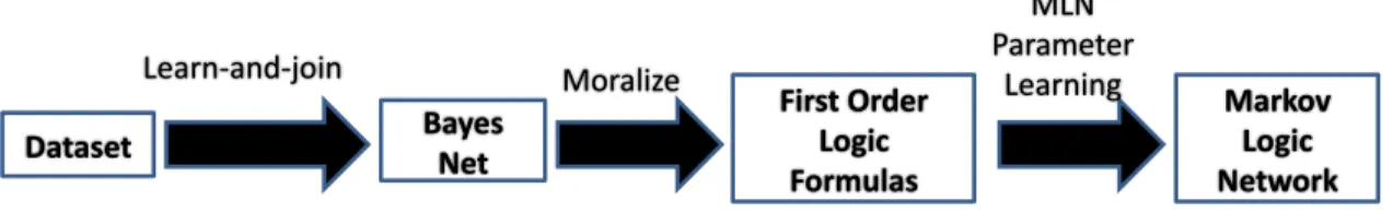
3.1 System architecture for learning a Markov Logic Network . . . 42

3.2 A Functor Bayes net graph for the relational schema of Table 2.1. . . 47

3.3 A lattice of relationship sets for the University schema . . . 48

3.4 The multinet lattice for the University Schema . . . 53

3.5 Hepatitis and MovieLens Bayes nets . . . 60

3.6 Accuracy by attribute, measured by 5-fold cross-validation . . . 67

3.7 CLL by attribute, measured by 5-fold cross-validation . . . 68

3.8 Rules of a given chain length for datasets . . . 71

4.1 Database instance and grounding . . . 75

4.2 A Functor Bayes Net and its grounding for the database of Figure 4.1 . . . . 76

4.3 The moralized Functor Bayes net of Figure 4.2 . . . 78

4.6 The 2-net lattice associated with the DB instance of Figure 4.1 . . . 87

4.7 University+ and Mondial datasets Bayes nets . . . 90

4.8 Percentage of rules of a given chain length for Mondial and University+ dataset 92 4.9 Dependencies discovered by the autocorrelation extension of the learn-and-join algorithm. . . 94

5.1 System Architecture for context-sensitive moralization . . . 97

5.2 A simple relational database instance for the relational schema of Table 5.1. 100 5.3 A Parametrized Bayes net graph for the relational schema of Table 5.1. . . . 101

5.4 Moralization . . . 101

5.5 A decision tree that specifies conditional probabilities for the ranking(S) node 103 5.6 join data table for learning a decision tree that represents the conditional probabilities ofranking(S) . . . 105

5.7 Decision tree learning . . . 106

5.8 The number of parameters learned using a Learning Curve scheme . . . 112

5.9 Weight learning time curve . . . 113

Introduction

Many databases store data in a relational format, with different types of entities and infor-mation about links among the entities. The field of statistical-relational learning (SRL) has developed a number of new statistical models for relational databases [33]. Markov Logic Networks (MLNs) form one of the most prominent SRL model classes; they generalize both first-order logic and Markov network models [15]. MLNs have achieved impressive perfor-mance on a variety of SRL tasks. Because they are based on undirected graphical models, they avoid the difficulties with cycles that arise in directed SRL models [79, 15, 105]. Es-sentially, an MLN is a set of weighted first-order formulas that compactly defines a Markov network comprising of ground instances of logical predicates. The formulas are the struc-ture or qualitative component of the Markov network; they represent associations between ground facts. The weights are the parameters or quantitative component; they assign a like-lihood to a given relational database by using the log-linear formalism of Markov networks. An open-source benchmark system for MLNs is the Alchemy package [61].

This dissertation addresses structure learning for MLNs in relational schemas that fea-ture a significant number of descriptive attributes compared to the number of relationships. Previous MLN learning algorithms do not scale well with such datasets. We introduce a new moralization approach to learning MLNs: first we learn a directed Bayes net graphi-cal model for relational data, then we convert the directed model to an undirected MLN model using the standard moralization procedure (marry spouses, omit edge directions)[15]. The main motivation for performing inference with undirected models is that converting a Bayes net to an undirected model avoids the cyclicity problem [15, 105, 53]. Thus our

approach combines advantages of both directed and undirected SRL models: learning effi-ciency and interpretability from directed models, and the solutions to the combining and cyclicity problems together with the inference power of undirected models.

1.1

Approach

We address three closely related research problems in this dissertation.

(1) In Chapter 3, we present a new algorithm for learning a non-recursive Bayes net from relational data, the learn-and-join algorithm. This algorithm performs a level-wise model search through the table join lattice associated with a relational database, where the results of learning on subjoins are propagated as constraints for learning on larger joins. This propagation mechanism leads to longer and more informative MLN clauses. A single-table Bayes net learner, which can be chosen by the user, is applied to each join table to learn a Bayes net for the dependencies represented in the table. For joins of relationship tables, this Bayes net represents dependencies among attributes conditional on the existence of the relationships represented by the relationship tables. The Bayes net is then converted to an MLN for inference using moralization. In our experiments on small datasets, the run-time of the learn-and-join algorithm is 200-1000 times faster than benchmark programs in the Alchemy framework [59] for learning MLN structure. On medium-size datasets, almost none of the Alchemy systems return a result given our system resources, whereas the learn-and-join algorithm produces an MLN structure within a few minutes. The structure of MLNs that are learned through moralization are more complex and use a combination of variables and constants, whereas other state-of-the-art MLN methods tend to learn a much sparser structure that only has variables. A preliminary version of this research was published in the proceedings of the Association for the Advancement of Artificial Intelligence (AAAI2010) conference [53]. Later a more detailed version was published in the Journal of Machine Learning [94]

(2) Chapter 4 focuses on recursive dependencies in relational data. A key phenomenon that distinguishes relational data from single-population data is that the value of an attribute for an entity can be predicted by the value of the same attribute for related entities; these are called recursive dependencies. For example, whether individualasmokes may be predicted by the smoking habits ofa’s friends. Conversion of Bayes nets to undirected models avoids cyclicity while performing inference; however, it still remains a problem for model selection

during the learning phase. The cycles make it difficult to define a model likelihood function for observed ground facts in the data, which is an essential component of model selection techniques. To define a model likelihood function for a Bayes net search, we utilize a recent relational Bayes net pseudo likelihood [93] that measures the fit of a Bayes net to a relational database and is well-defined even in the presence of recursive dependencies. To show recur-sive dependencies using this pseudo likelihood, additional copies of variables participating in the recursive dependencies are added to the graphical model. For example a second variable to show the smoking habits of users is added to the graphical model. This pattern can be represented by a clausal notation such as Smokes(X) ← Smokes(Y),Friend(X,Y). If each replicated predicate is treated as a separate random variable, then multiple redundant edges showing the same dependency will be added, as the logical variables are interchange-able placeholders for the same domain of entities. In this chapter we propose a normal form for Bayes nets that are learned from relational data to eliminate such redundancies and prove that this constraint incurs no loss of expressive power. A preliminary version of this research was published in the proceedings of the Inductive Logic program (ILP2011) conference [97]. Later a more detailed version was published in the Journal of Machine Learning [98]

(3) In Chapter 5 we learn compact Markov Logic Networks using decision trees. A weakness of the moralization approach is that it leads to an unnecessarily large number of clauses. The Bayes net method learns dependencies among predicates, not literals, which fail to capture local or context-sensitive independencies. MLNs have one weight parameter for each clause, which decreases the accuracy of parameter estimates, and slows down inference. In this chapter, we show that using decision trees to represent conditional probabilities in the Bayes net is an effective remedy that leads to much more compact MLN structures. The decision trees can be learned using standard propositional decision tree learners. In experiments on benchmark datasets, the decision trees reduce the number of clauses in the moralized MLN by a factor of 5 to 25, depending on the dataset. The accuracy of predictions is competitive with the unpruned model and in many cases superior. A preliminary version of this research was published in the proceedings of the Inductive Logic program (ILP2011) conference [51]. Later a more detailed version was published in the Journal of Machine Learning [52]

1.2

Contributions

The main contributions of this dissertation are the following:

1. A new structure learning algorithm, learn-and-join, for Bayes nets that models the distribution of descriptive attributes given the link structure in a relational database with discussion and justification for some relational constraints that speed up structure learning. The algorithm is a level-wise lattice search through the space of join tables. 2. A new normal form theorem for Bayes nets that addresses redundancies in modelling

recursive dependencies.

3. An extension of the learn-and-join algorithm for learning Bayes nets from relational data that include autocorrelations.

4. A new structure learning algorithm augmenting Bayes net learning with decision tree learning to learn a compact set of clauses, a Markov Logic Network, for relational data.

5. A comparison of all of our proposed methods with other state-of-the-art methods.

1.3

Limitations

The main limitations of the work presented in this dissertation are the following:

1. Our current algorithms do not find associations among relationships. For instance, if a professor advises a student, then they are likely to be coauthors. In the terminology of Probabilistic Relational Models [30], our model addresses attribute uncertainty, but not existence uncertainty (concerning the existence of links).

2. In this dissertation, we only focus on learning the structure, and we use the default Markov Logic Network method provided in the Alchemy package for parameter learn-ing. While this parameter learning method finds suitable parameter settings, it is slow and constitutes the main computational bottleneck for our approach. In our experiments, 98% of the time for learning is spent optimizing the parameters for the learned structure. We propose a moralization approach to parameter estimation where MLN weights are directly inferred from Bayes net parameters. Empirical evaluation

indicates that parameter estimation via moralization is orders of magnitude faster than parameter optimization, while performing as well or better on prediction met-rics. This research is not included in this dissertation, and appears in the proceedings of the Inductive Logic Programming conference [49].

3. In this dissertation, we do not discuss any industrial applications for the learn-and-join algorithm; the learned Bayes nets are always converted to Markov Logic Networks for inference on the ground model. The standard grounding semantics is appropriate for answering queries about individual ground facts (“What is the probability that Tweety can fly?”) but not appropriate for answering frequency queries (“What is the probability that an arbitrary bird can fly?”), because frequency queries concern generic events. Frequency queries may be used for query optimization, policy making and strategic planning, and finding statistical first-order patterns. To apply Bayes nets to such queries we propose a frequency semantics for Bayes nets, based on Halpern’s classic domain frequency semantics for probabilistic first-order logic [36]. Learning the parameters for such a frequency semantics can be done using our learn-and-join algorithm which like Halpern’s semantics is based on random instantiations of first-order variables. A naive computation of the empirical frequencies of the relations is intractable due to the complexity imposed by negated relational links. We render this computation tractable by using the fast Moebius transform. This research is not included in this dissertation and appears in the proceedings of the Inductive Logic Programming conference [96].

Background and Literature Review

In Section 2.1, we provide the necessary background on fields related to this dissertation. The rest of this chapter provides a literature review and a running example on some of the state-of-the-art models in statistical relational learning; the methods of representing, learning, and inference are discussed. In Section 2.2, we discuss Probabilistic Relational Models; their graphical model is very similar to that of ours. In Section 2.3 we discuss Markov Logic Networks; the main contributions of this dissertation are learning methods for learning Markov Logic Networks. In Section 2.4 we discuss Relational Dependency Networks and in Section 2.5 we discuss Bayesian Logic Programs. We conclude this chapter with Section 2.6 which addresses the limitations of current models and provides a comparison among them.

2.1

Background and Notation

In this section we introduce some notation and terminology that is referred to throughout this dissertation. Please consider reading the citations in case you need more familiarity with any of the topics discussed. We presents a brief discussion on probability, logic, machine learning, Bayesian networks, decision trees, relational data, and relational models in this section.

2.1.1 Probability Distribution

We assume general familiarity with probability theory. We denote random variablesby capital letters (X,Y,...) and the values of a random variable by lower case letters (x,y,...). We denote sets of random variables by boldface capital lettersX={X1, . . . , Xn}.

The set of values of a variable is therange of the variable. In this dissertation we only consider random variables with a finite range. We write P(X1 = x1, ..., Xn = xn) = p,

sometimes abbreviated as P(x1, ..., xn) = p, or P(X = x) = p, to denote that the joint probability of random variables X1, . . . , Xn taking on values x1, . . . , xn is p. The sum of

the joint probability distribution of a set of random variables X over all possible values x is 1, that is,

X

x

P(X=x) = 1

The joint probability distribution of a subset Y of X can be obtained by summing out the remaining variables Z= X\Y. The distribution is called the marginal probability distribution ofY.

P(Y) =X

z

P(Y,Z=z)

The conditional probability of a subset (Y) ∈ (X) given a subset Z ∈ (Z) is the probability of Y occurring when we know Zhas occurred. The conditional probability can be obtained by the following formula:

P(Y|Z) = P(Y,Z)

P(Z)

Two eventsX andY areindependent if occurrence ofX does not effect the probability of Y occurring. In such a event, the joint probability of the two events co-occurring is calculated by the product of each of their occurrence:

P(X,Y) =P(X)×P(Y)

2.1.2 Logic

We assume general familiarity with propositional and first order logic. In this dissertation, a termτ is a constant or a variable. Afunctor is a function symbol. Each functor has a set

of values (constants) called therange of the functor. A functor whose range is{T,F}is a predicate, usually written with uppercase letters likeP, R. Afunctor random variable is of the formf(τ1, . . . , τk) wheref is a functor and eachτiis a term. We also refer to functor

random variables as functor nodes, or for short fnodes.1 Unless the functor structure matters, we refer to a functor node simply as a node. If functor node f(τ) contains no variable, it isground, or a gnode. If functor node contains a variable, it is a vnode.

An assignment of the formf(τ) =x, wherexis a constant in the range off, is aliteral; iff(τ) is ground, the assignment is aground literal. Apopulationis a set of individuals, corresponding to a domain or type in logic. Each first-order variableX is associated with a populationP_X of size|P_X|; in the context of Functor Bayes nets, we refer to population variables[84]. An instantiationorgroundingγ for a set of variablesX1, . . . , Xkassigns

a constantγ(Xi) =xi from the population ofXi to each variableXi.

2.1.3 Machine Learning

Machine learning has become a crucial part of computer science; as a broad subfield of artificial intelligence, machine learning is concerned with the design and development of algorithms and techniques that, given a dataset D and an objective function f(.), search through the hypothesis space or models M for the most suitable candidate m ∈ M such thatf(m,D) is maximized.

A variety of machine learning tasks may be distinguished by the characteristics of the hypothesis space (models) considered and the objective function. In this dissertation we address the following.

• Discriminative Learning is a class of learning in which the objective functionf(.) is de-fined as to maximize the predictive performance of the model on a target attributeT, for unseen data. The output is usually a conditional probability distribution P(T|E) over the range of the values of T where E is the evidence information from other attributes. Decision Trees, discussed in Sec 2.1.5, are a well known model for discrim-inative learning.

• Generative Learning is a class of learning that aims to model and describes the patterns

1_{The term “functor” is used as in Prolog [7]. In Prolog, the equivalent of a functor random variable is} called a “structure”. Poole [84] refers to a functor random variable or fnode as a “parametrized random variable”. We use the term fnode for brevity.

and regularities in the data. The output is usually a probability distribution over the random variables in the model. Bayesian Networks, discussed in Section 2.1.4, are a well known model for generative learning.

2.1.4 Bayesian Networks

We employ notation and terminology from [83, 101] for a Bayesian Network. We consider Bayes Nets for a set of variables V = {X1. . . Xn} where each Xi has a finite range. A Bayes net structureG= (V,E) for a set of variablesVis directed accylic graph (DAG). ABayes net(BN) is a pairhG,θGiwhereθG is a set of parameter values that specify the

probability distributions of children conditional on assignments of values to their parents. The conditional probabilities are specified inconditional probability tables.

If X, Y are two variables and S is a set of variables disjoint from {X, Y}, then S d-separates X and Y if along every path between X and Y there is a node w satisfying one of the following conditions: (1) w is a collider on the path and none of w nor any of its descendants are in S, or (2) w is not a collider on the path and w is in S. We write (X ⊥⊥ Y|S)G if X and Y are d-separated by S in graph G. If two nodes X and Y are

not d-separated by S in graph G, then X and Y are d-connected by S in G, written (X⊥6⊥Y|S)G. If X,Y and Zare three disjoint sets of variables, then Zd-separates X and Y if for all variablesX ∈X and Y ∈Y, the setZd-separates X and Y.

For a node X, we refer to the set of its parents, children and co-parents (i.e. other parents of its children) as the Markov blanketofX,M B(X). Given its Markov blanket, each nodeX in G is d-separated from all other nodes outside of the Markov blanket. We refer to the set of independences{X⊥⊥Y|M B(X) :Y 6∈M B(X)} as the set of Markov blanket independencesfor graphG.

Figure 2.1 is a well known example of a Bayesian network from [92]. In the example, the event of grass being wet has two possible causes: either the water sprinkler is on, or it is raining. Cloudy weather causes rain and reduces the probability of sprinkler being on. The strength of the relationships are given in the conditional probability tables.

Learning Bayesian Networks

Given a set of variables V and a dataset D containing independent and identically dis-tributed (i.i.d) examples from an unknown distributionP, the goal of structure learning is

Figure 2.1: An example of a Bayesian network taken from [92].

to identify a directed acyclic graph G that represents P. Finding an optimal structure is a computationally intractable problem; structure learning algorithms determine for every possible edge in the network whether or not to include the edge in the final network and which direction to orient the edge. The total possible number of graphs is super exponential in|V|. Even a restricted form of structure learning where variables are constrained to have at most k parents has been proven to be NP-Complete. Two broad classes of structure learning are well-known in the literature [76, 37].

• Score Based methods search over possible Bayesian network structures for the most suitable factorization of the joint probability based onD. The model selection criterion is usually defined as a score that the methods are trying to maximize. BDeu [38] and BIC [11] are examples of well known scores for Bayesian network learning.

• Constraint Based methods employ a statistical tests to detect conditional (in)dependencies given a sample D, and then compute a BN structureG that fits the (in)dependencies [68, 10]. The (in)dependencies test can be chosen to suit the type of available data and application domain. One of the traditional test for categorical data is the χ2 test. To form a complete Bayes net, an additional step of parameter estimation is required to determineθGfromD. Since the focus of this dissertation is on structure learning, techniques

Parametrized Bayes Nets

Parametrized Bayes nets(PBNs) were introduced by Poole to study first-order probabilistic inference on directed models. They are a comparatively simple adaptation of the Bayes net format for relational data. The syntax of PBNs is similar to that of other directed graphical SRL models, such as Bayes Logic Programs [46] and Probabilistic Graphical Models [26]. A Parametrized Bayes Net structure consists of: (1) a directed acyclic graph whose nodes are functor nodes. (2) a population for each first-order variable. (3) an assignment of a range to each functor. A Parametrized Bayes Net is a Bayes net whose graph is a parametrized Bayes Net structure. Because each of the nodes in a parametrized Bayes net is a functor, We also use the name Functor Bayes Nets (FBNs) for them.

2.1.5 Decision Trees

A decision tree is a discriminative method for predicting a target attribute using a tree. We consider decision trees for a set of variables V= {X1. . . Xn, T} where T is the target

attribute and each Xi and T have a finite range. An instance{x1. . . xn, t} is classified by

starting at the root node of the tree. EachXi nodes in the tree specifies a test on the value xi; a branch is selected based on xi. This process is then repeated for the subtree rooted

at the next node. Each branch is terminated with a valuet in the range of T which is the classification value. Figure 2.2 is a well known example of a decision tree from [71]. The model decides if the weather is amenable for playing tennis. It illustrates that in case of sunny outlook and normal humidity tennis will be played and in case of rainy outlook and strong wind, tennis will not be played.

Learning Decision Trees Most algorithms that have been developed for learning de-cision trees are variations of the ID3 algorithm [89] by Quinlan that employ a top down greedy search through the space of possible trees. As in any greedy algorithm, a definition for the best choice is required; each of the attributes, on its own, is used to build a classifier of depth one, and is evaluated on the training. This is equivalent to selecting the attribute with the smallest entropy measure on the training set. The best attribute Xi is selected

and used as the root node of the tree. A descendant node of the root is generated for each

xi. This process is repeated until an ending criterion is met.

2.1.6 Relational Data and Databases

The majority of work in learning has focused on data which consists of identically struc-tured entities that are assumed to be independent. However, many real world datasets are relational and most real world applications are characterized by the presence of uncertainty and complex relational structure; statistical learning is based on the former and relational learning is based on the latter.

Statistical relational learningis a new branch of machine learning that aims to model a joint distribution over relational data. Relational data are more complex and better suited where examples are given as multiple related tables. The structure of relational data presents an opportunity for objects to carry additional information via their links and enables the model to show correlations among entities and their relationships [33].

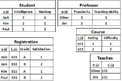
We assume general familiarity with relational databases [107]. We use standard relational schema containing a set of tables, each with key fields, descriptive attributes, and foreign keys. A table join of two or more tables contains the rows in the Cartesian products of the tables whose values match on common fields. If the schema is derived from an entity-relationship model (ER model) [107, Ch.2.2], the tables in the relational schema can be divided into entity tables and relationship tables. Table 2.1 shows a example of a university relational schema. The entity types of schema of Table 2.1 are students, courses and professors. There are two relationship tables: Registration records courses taken by each student and the grade and satisfaction achieved, andRArecords research assistantship contracts between students and professors. Relationships refer to their related entities using reference slots. Each table in the relational database is considered as a class with some descriptive attributes.

Student(student id,intelligence,ranking) Course(course id,difficulty, rating)

Professor (prof essor id, teaching ability, popularity) Registered (student id, course id, grade, satisf action) Teaches(professor id,course id)

Table 2.1: A relational schema for a university domain. Key fields are underlined.The schema has three entities and two relationships

schema. Figure 2.3 illustrates a database instance for schema in Table 2.1

Figure 2.3: A database instance for schema in Table 2.1.

The functor syntax is rich enough to represent an entity-relation schema [107, Ch.2.2] via the following translation: Entity sets correspond to populations, descriptive attributes to function symbols, relationship tables to predicate symbols, and foreign key constraints to type constraints on the first-order variables.

We assume that a database instance assigns a unique constant value to each gnodef(a). The value of descriptive relationship attributes is well defined only for tuples that are linked by the relationship. For example, the value of grade(jack,101) is not well defined in a university database ifRegistered(jack,101) is false. In this case, we follow the approach of Schulteet al. [95] and assign the descriptive attribute the special value⊥ for “undefined”. Thus the atom grade(jack,101) =⊥implies Registered(jack,101) =F. Fierens et al. [20] discuss other approaches to this issue. The results in this paper extend to functors built

with nested functors, aggregate functions [55], and quantifiers; for the sake of notational simplicity we do not consider more complex functors explicitly.

It is possible to represent relational data using a graph GD(VD, ED) where the nodes of GD are the entities of the database and the edges between them represent the relationships between the entities. A vector is assigned to each of the nodes and edges to keep the information of the attributes of the entity and the links. Figure 2.4 shows GD(VD, ED) for

the instance in Figure 2.3

Figure 2.4: Graph GD(VD, ED) for the instance given in Figure 2.3. The nodes represent the entities of the schema and the links represent the relationships. An array is assigned to nodes and edges that carries the information of the objects and the relationships.

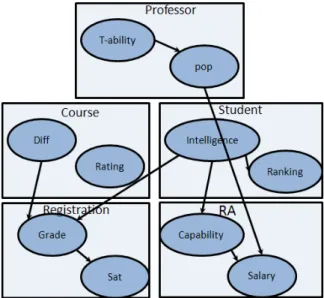
Graphical models [64, 45] have become a popular tool for modeling statistical relational models, and provide a principled approach to dealing with uncertainty and relational data through probability theory. The goal of graphical models is to represent a joint distribution. It encodes probabilistic relationships over a set of random variables. The graphical structure of the model is used to present the independence that exist among variables. The two most common classes of graphical models are Bayesian networks, which are directed graphs and Markov Networks, which are undirected graphs [83]. In this section we use GM(VM, EM)

to represent the first-order class template of the methods discussed. Figure 2.5 shows an example of aGM(VM, EM) for the instance in Figure 2.3.

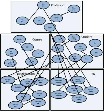
Learning graphical models for relational data is very slow due to model selection. To perform model selection in structure learning for a modelm∈ M, a new graphGI(VI, EI) is produced, by rolling outGD overm. GI(VI, EI) takes the template frommand the relations

in GD(VD, ED) constrains the way it is rolled out. Gi is called the ground model and is generated with the property that there is a node for every attribute of each object and the parameters of the models for attributes of the objects are inherited from m. GI evaluates how wellmmodelsGD. Figure 2.6 shows an example. With this model selection technique,

Figure 2.5: An example of a graphGM(VM, EM) forGD given in Figure 2.4. The variables

represent descriptive attributes of tables of the schema and edges show dependencies between attributes.

of each table, but also dependencies among attributes of different tables. For example, a statistical relational model may show that intelligence of a student and difficulty of a course are related to the grades achieved by the student.

Learning graphical models for relational data is much more challenging than learning graphical models for propositional data. The following are some of major differences of relational data amd propositional data.

• Propositional data consists of identically structured entities, typically assumed to be independently and identically distributed (iid); however relational data consists of different entities of different types which may be related to each other.

• In propositional data, learners model a fixed set of attributes intrinsic to each object, whereas in relational data, learners decide on what information to use in their model as the links of the linked objects may also carry helpful information. Collective inference [44] consider the links of the linked objects as well as just the links of the object. • In modeling propositional data, the number of states is exponential in the number of

attributesO(2n). For relational data, theGI graph hasn×mvariables wherenis the

Figure 2.6: The graph GI for GM in Figure 2.5 rolled out over the schema in Figure 2.4. The variables of the graph show descriptive attributes of each object and edges connect attributes of objects using the template fromGM

of GI is exponential in the product of the attributes and objectsO(2nm).

• Correlations between values of attributes of objects of the same type were dubbed autocorrelations by Jensen and Neville [12]. Let Abe an attribute of an entityE and

e1 ande2 are instances of typeE. A relationship between objects of the same entity is

required to have autocorrelation. Assume R(E,E) is a relationship on entity E where

R(e1, e2) =T. There well may be a correlation between the attribute valueA(e1) and

the attribute value A(e2). A well known example for autocorrelation it that, the gene

type of a child is correlated to the genes of his parents. The presence of autocorrelation is a feature of relational data which increases the complexity of relational learning. • We call two tables T1 and T2 related if T2 is a relationship table with foreign key

pointer to entity table T1, or T1 and T2 are both relationship tables with foreign key

pointers to a common entity table E1. Let X1, Y1, .., Yk, , X2 fork > 0 be attributes

associated with a database schema. The variables form a slot chain if neighboring variables are related; for example, Y1 = grade in the Registered table forms a slot

chain forX1 =intelligence and X2 =difficulty. Correlations through a slot chain are

also a feature of relational data and are challenging to discover.

• A difficulty with modeling relational data is that the database may contain information about many links related to an entity that need to be combined. For instance, a Bayes net may encode the probability that a student is highly intelligent given the properties of a single course they have taken. But the database may contain information about many courses that the student has taken, which needs to be combined; we may refer to this as the combining problem.

The presence of relational data not only leads to more accurate results on traditional tasks like classification and prediction, but also introduces some new tasks that have at-tracted the interest of many researchers. Popular tasks defined for SRL models include the following.

• Collective classification [44] is an extension of relational classification. Relational classification is the task of predicting the class of an object given its attributes, links, and other objects that are related through its links. In collective classification, the links of related objects are also considered for classification.

• Linked-based clustering [110] groups together objects that have similar characteristics both in their own attributes [23] and more importantly in the attributes of their links • Link prediction [104] determines whether a relation exists between two objects from

the properties of the objects and their links.

• Entity resolution is the problem of determining which records in datasets refer to the same objects in the real world [113]

In the remainder of the chapter we review four of the proposed models in statistical rela-tional learning in details; the methods of representing, learning, and inference are discussed on a running example.

2.2

Probabilistic Relational Models(PRMs)

Probabilistic Relational Models (PRMs) [26] are a rich representation language for statisti-cal models. PRMs were one of the first successful methods proposed for statististatisti-cal relational learning. They use a Bayesian network as their framework and combine logical represen-tation with probabilistic semantics. PRMs extend Bayesian networks with the concept of objects. A PRM and a database instance define a probability distribution over the de-scriptive attributes of the objects and the relationships. In this section we will review the representation, learning, and inference methods for PRMs.

2.2.1 Representation in PRMs

PRMs define a probability distribution for a relational skeleton, a partial specification of an instance of the schema where the relations are defined but the descriptive attributes of the entities and relationships are undefined. A PRM, like a Bayesian network, has two components: the dependency structure and the parameters associated with it. Random variables in PRMs can have two types of dependencies, (1) both variables correspond to attributes from the same table, and (2) variables correspond to attributes from different tables but there is a slot chain between them. The second type of dependency is usually between a value and a set which is an example of the combining problem. PRMs use the notion of aggregation from database theory to return a summary in one value. There are many functions used as aggregation of a set: mode, mean, median, maximum, and minimum are among the most used aggregation functions. Figure 2.5 shows a class levelGM(VM, EM) for the instance in Figure 2.3.

A massive Bayesian network, GI, serves as the ground model for PRMs. Figure 2.6 shows a ground Bayes net for the instance given in Figure 2.3. As with a normal Bayesian network, an acyclic network guarantees coherence of the probability model.

PRMs with structural uncertainty

The previous section described PRMs with uncertainty over just the descriptive attributes of entities and relationships. However, PRMs can be extended to allow uncertainty over the relationships between objects. They can define a probability distribution for anobject skeleton, a relational skeleton where the relationship tables exist, but the reference slots are not assigned. For example the Student, Course and the Registered table are specified but

the student id and course id in the registration table are unassigned. Thus they need to specify a probability distribution over all objects in the entity tables for the reference slots. Since there are many objects, assigning a probability over each object is neither useful nor practical. To achieve a general and compact representation, they use the values of some descriptive attributes of entities to partition the distribution of objects. Acyclic PRMs with reference uncertainty relative to an object skeleton define a coherent probability distribution over instantiations extending the object skeleton.

The second form of structural uncertainty introduced by PRMs is existence uncertainty in which they further limit the background information. In reference uncertainty the number of tuples in both entity and relationship tables is known. In existence uncertainty the total number of links in relationships is unknown, so each potential link can be present or absent. The only input is anentity skeleton, which specifies the set of objects of the domain only for the entity classes. In existence uncertainty for each relationship, a binary attribute with values true and false is added to the list of descriptive attributes. The existence node, like any other node, can have parents and children, and there is a conditional probability table assigned to it. To make the model coherent and consistent, PRMs add the following conditions to the model.

1. Suppose that relationR has slots p1, ..., pk. The conditional probability table for the

added node is filled regularly if all the slots are true and 0 otherwise.

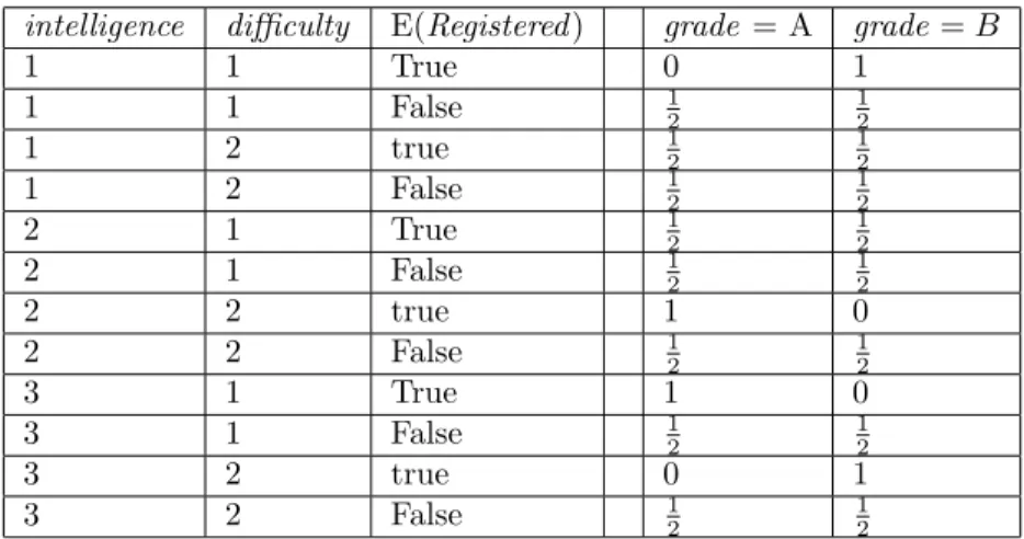
2. If the binary attribute is a parent of a descriptive attribute ofR, the conditional prob-ability table of the descriptive attribute is filled regularly when the binary attribute is true and is a uniform distribution on all possible values in the domain of A if E(R)= False. For example, the conditional probability table for attributegrade given that it has three parentsintelligence,difficulty, andB(Registered) is given in Table 2.2. The probability for rows where B(Registered)= False is 1₂ in this example. Rows where E(Registered)= True is calculated using look ups inRegistered, Student, andCourse tables in Figure 2.3.

2.2.2 Inference in PRMS

PRMs in few cases, when either the skeleton is small or the tree width is low, can use exact inference on theGI(VI, EI) graph. Unfortunately exact inference is usually not applicable

intelligence difficulty E(Registered) grade = A grade=B 1 1 True 0 1 1 1 False 1₂ 1₂ 1 2 true 1₂ 1₂ 1 2 False 1 2 1 2 2 1 True 1₂ 1₂ 2 1 False 1₂ 1₂ 2 2 true 1 0 2 2 False 1₂ 1₂ 3 1 True 1 0 3 1 False 1₂ 1₂ 3 2 true 0 1 3 2 False 1₂ 1₂

Table 2.2: The conditional probability table for attribute grade when a binary node B(registration) is in the set of parents of grade.

with real world data. Inference in PRMs requires inference over the ground network defined by an instantiated PRM for a specific skeleton. Because GI(VI, EI) is usually very large,

efficient inference is very complicated. The approximate algorithm used for inference in PRMs is a variant of belief propagation. We briefly describe the algorithm but for more information see [73, 111]. A Bayesian network can be converted into a family graph where a node is added for the set of every node and its parents, and an edge is added between nodes if they have common variables. If some new evidence is observed in the Bayesian network it may effect all the other nodes that are dependent on the observed node. The family graph is structured in a way that all of the dependent nodes in the Bayesian network are d-connected. So, a parameter passing algorithm can update all effected nodes by passing the new information through its edges. While the algorithm is not guaranteed to converge, it typically does so after several iterations.

2.2.3 Learning In PRMs

We will review parameter learning and structure learning in PRMs briefly. Parameter Learning

The key feature in parameter learning is the likelihood function which is defined as the probability of the data given the model. LetGX_D(a) be an assignment of values of object a

the probability of the data given the model for PRMs. l(θGM|GD, GM) = X X∈VM X a∈a logp(GX_D(a)|Gpa(X)_D (a)) (2.1) WhereθGM is the parameters forGM,ais the set of objects. An important component of learning is the score function. A score is decomposable if it can be calculated by independent summations over the score of the nodes of the structure [37]. Decomposability of the score has significant impact on the efficiency of the algorithm. To perform parameter learning using a decomposable score, PRMs use the well established maximum likelihood parameter estimation. Using Maximum Likelihood, Formula 2.1 can be decomposed into summation terms that each may be maximized separately,

l(θGM|GD, GM) = X X∈VM X x∈X X u∈pa(X)

C_[x,u]×logθ_GM(x|u) (2.2)

whereC_[x,u] is the number of times GX_D(a) =x and Gpa(X)_D (a) =u. v|u is the conditional probability ofGX_D(a) =v given G_Dpa(V)(a) =u.

An important advantage of using a relational database is that SQL queries may be used to calculate local probabilistic distributions and sufficient statistics. For example the statis-tics for intelligence of students, their grades and capabilities from theRegistered and theRA table can be computed respectively,SELECTcapability, intelligence, grade, count(*) FROMRegistered,Student,Course,Professor,RA

WHERERegistered.student id=Student.student idandRegistered.course id=Course.course id

andRA.student id = Student.student id and RA.prof essor id= Professor.prof essor id

GROUP BYcapability, intelligence, grade

In cases where an attribute in the set of the parents is from a different tables, a view is used to reduce the computation cost. To compute the correct statistics, the projection and the group by commands in SQL may be used on the created view. SQL also supports most of the aggregation functions used by PRMs.

Structure Learning

Structure learning is more challenging than parameter learning in graphical models. The general task of structure learning is to find the set of edges EM in GM. The “goodness”

For evaluating different structures, score functions like BIC [37] as described in Section 2.1.4 are used. As BIC and most other score functions are only defined for (iid) data, a new definition for these scores must be specified for use of relational data. Generally for Bayesian networks, the task of finding the best structure is NP hard. PRMs use greedy algorithms that iteratively modify the structure to increase the score. The operations used in each step are adding, removing or reversing an edge. Adding or reversing an edge may introduce cycles but it is possible to check a PRM for cycles inO(|VM|+|EM|). In each step, all possible transformations using these operations are considered and the transformation with the best score is selected. Greedy algorithms often get stuck in local maximums. PRMs consider a number of random operations and then restart the greedy search process to avoid this problem. Greedy methods become more efficient if a tabulist is used to keep tack of visited states, so the search algorithm does not return to a recently visited state. Also, operations used in PRMs structure learning only change the parents set of maximum of two nodes on the sides of the modified edge. By using a decomposable score, only the components of the score associated with these two nodes need to be reevaluated.

Learning With Reference Uncertainty To cover learning with reference uncertainty PRMs need to define the partitions which involves expanding search operators to allow ad-dition and deletion of attributes in the partition function. PRMs with reference uncertainty need to introduce two new operators refine and abstract. The partitions can be defined using a decision tree whererefine adds a split to one of the leaves to make the result more specific andabstract removes a split to make the partitions more general.

Learning With Existence Uncertainty Extending PRMs with existence uncertainty is straightforward. The existence attribute is treated the same as descriptive attributes. The new concept is how to compute sufficient statistics that include existence attributes without explicitly enumerating the non existent entities. To do so PRMs count the number of potential objects with a given instantiation from entity tables and subtract the actual number of true objects that have been instantiated from relationship tables. No new op-erations are added to handle existence uncertainty but PRMs force additional edges in the class dependency graph.

2.3

Markov Logic Networks(MLN)

Markov Logic Networks (MLNs) [15] are among the most well known methods proposed for statistical relational learning. They have been introduced as a unifying framework for SRL to facilitate transfer of knowledge across approaches, make comparison and understanding of different models easier, and help establish structure to the field. The authors mention several criteria for the unifying framework. First, the framework must be consistent with first-order logic and probabilistic graphical models as many current approaches rely on them. Second, the framework must be clear and simple. Finally, the framework must facilitate the use of domain knowledge in statistical relational models.

Essentially, an MLN is a set of weighted first-order formulas that compactly defines a Markov network comprising ground instances of logical predicates. The formulas are the structure or qualitative component of the Markov network; they represent associations between ground facts. The weights are the parameters or quantative component; they assign a likelihood to a given relational database by using the log-linear formalism of Markov networks. An open-source benchmark system for MLNs is the Alchemy package [61].

2.3.1 Representation in MLNs

MLNs combine first order logic and Markov networks. A Markov network is a model for the joint distribution of a set of variablesX = (X1, X2, . . . Xn). It is composed of an undirected

graphGand a set of potential functionsφk. The graph has a node for each variable, and the

model has a potential function for each clique in the graph. A potential function is a non-negative real-valued function of the state of the corresponding clique. The joint distribution represented by a Markov network is given by

P(X=x) = 1

Z Y

k

φk(x{k}) (2.3)

where (x{k}) is the state of the kth clique. Z, known as the partition function, is given by

Z=P

x∈X Q

kφk(x{k})

A first order knowledge base is a set of hard constraints where if a grounding violates just a single formula, the probability of its happening is zero. This hard constraint in first order logic makes them inappropriate for modeling noisy data or datasets with contradicting rules. Markov logics extend first-order logic so that the hard constraints are replaced with soft

First-order logic Weight English

∀x(intelligent(x)⇒highrank(x)) 2.3 If a student is intelligent

then his rank is high ∀x∀y(intelligent(x)∧f riend(x, y)

0.7 If a student has an intelligent

⇒ intelligent(y)) friend then he is intelligent

Table 2.3: Example of a small MLN

constraints using formulas that have weights based on the importance of the constraint. In MLNs, if a grounding violates some formulas, it is just less probable. The fewer groundings a formula violates, the more probable the formula is.

Formally, a Markov Logic Network is a set of pairs of formulas and their corresponding weights (Fi, wi) where formulas are in first order logic and the weights are real numbers. The set of formulas in MLNs correspond to the class modelGM. An MLN with a finite set

of objects in GD defines a ground Markov network GI which has a binary node for each ground predicate in the MLN. The value of the node is 1 if the ground atom is true and 0 otherwise. An MLN is a template for the ground Markov network and the size of the model is a function of the number of objects. The structure and the parameters of the ground network are forced by the MLN model. The edges are cliques between ground atoms that appear together in a formula and all groundings of a the same formula have the same weight as specified by the MLN.

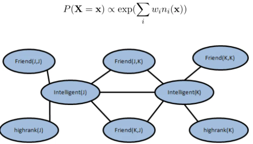
Table 2.3 presents an MLN for the university example. The MLN has two formulas for the students. One of the formulas connects intelligent and highrank and the other one connects f riend and intelligent. Assuming there are only two students Jack (j) and Kim (k) in our university, Figure 2.7 shows the ground Markov network GI for the MLN

in Table 2.3. Edges between f riend predicates and intelligent predicates are due to the second formula and edges between intelligentpredicates and highrank predicates are due to the first formula.

Each state of the Markov network represents a database instance. The probability distribution over database instancesx specified by the ground network is calculated by

P(X=x) = 1

Z exp(

X

i

wini(x)) (2.4)

where ni(x) is the number of true groundings for Fi in x and Z is the partition function

out the denominator, the likelihood is calculated using Formula 2.5

P(X=x)∝exp(X

i

wini(x)) (2.5)

Figure 2.7: Ground Markov network obtained by applying MLN of Table 2.3 to Jack and Kim

To show an example of calculating probabilities for possible database instances, we further simplify the example. Suppose that the MLN has just the first formula in Table 2.3 and Jack is the only student. This leads to four database instances:

1. {intelligent(J), highrank(J)}

2. {intelligent(J),¬highrank(J)}

3. {¬intelligent(J), highrank(J)}

4. {¬intelligent(J),¬highrank(J)}

Using Formula 2.5, the likelihood forP(X ={¬intelligent(J), highrank(J)}) = 1 and the likelihood for the other three instances ise2.3. As the probability of all database instances needs to add up to 1, _Z1 can be calculated. Formula 2.6 computes the inverse of the potential function of our example.

1

Z =

1

3e2.3_{+ 1} (2.6)

so P(X = ¬intelligent(J), highrank(J)) = _3e2.13₊₁ and probability of the other three

instances is _3ee22.3.3₊₁. The probabilities indicate that instances that are inconsistent with the

2.3.2 Inference in MLN

In this section we discuss how inference is performed in MLNs. The sort of queries that may be answered using an MLN are of the form “What is the probability that Fi1 holds knowing that Fi2 holds, given the ground Markov network”. This may be formalized as

P(Fi1|Fi2, GI(VI, DI)). Inference in MLNs is done on the ground Markov network; a brute

force way of calculating this probability is by using formula 2.7.

P(Fi1|Fi2, M) = P(Fi1, Fi2|M) P(Fi2|M) = P x∈(x_Fi 1∩xFi2) P(X=x|M) P x∈x_Fi 2 P(X=x|M) (2.7) xF i is the set of instances where Fi holds. This direct inference method is highly

in-tractable and is only applicable to very small domains. Inference in Markov networks itself is generally NP complete and cannot be carried out on networks with many nodes. So, a different method of inference is used in MLNs. The approach has two main phases.

In the first phase a minimal subset ofGI, the ground Markov network, that is required

for computingP(Fi1|Fi2, M) is obtained. Many predicates that are irrelevant toFi1 andFi2

may be filtered in this phase. As a result, a smaller Markov network is used for inference. In the second phase, we perform inference on the Markov network using Gibbs sam-pling [8] where the nodes of Fi2 are observed and are set to their values. In Gibbs sam-pling the unobserved variables in the network are randomly initialized and ordered to

{X1 = x1, . . . , Xn = xn}. In step 1 a new value x01 for variable X1 is sampled

condi-tional on all the other variables P(X1|X2 =x2, . . . , Xn=xn), and in stepi a new valuex0_i

for variable xi is sampled conditional on all the other variables P(Xi|X1 = x01. . . Xi−1 =

x0_i−1, Xi+1 =xi+1. . . Xn =xn). We can take advantage of the conditional independence to

ease the computation. Conditional on its immediate neighbors, Markov Blanket, a node is independent of all of the other variables. Assuming M B(Xk) = b = {b1. . . bi} shows the

different states of the Markov blanket of the node Xk, the probability of a ground atom X=x given its Markov blanket is in statebl is

exp(P fi∈FlwiFi(x, bl)) exp(P fi∈FlwiFi(X = 0, bl)) + exp( P fi∈Flwifi(X= 1, bl)) (2.8) where Fl is the set of ground formulas thatX appears in, and fi(X = 1, M B(X) = bl) is

the value corresponding toFi when it has been grounded byX= 1, M B(X) =bl. To make

While transferring an MLN to a Markov network, some undesired cliques may be gener-ated that do not correspond to groundings ofFis; the Markov network contains some spuri-ous cliques that should not be involved in computing probability distributions of database instances. Therefore, the MLN is required for guidance and the Markov network can not be used on its own for inference.

2.3.3 Learning in MLN

Having efficient structure and parameter learning algorithms is crucial for any graphical model. Without efficient learning algorithms, the model is unsuitable for realistic size do-mains and problems. Learning is a hard task in Markov networks; in this section, parameter learning for MLNs is discussed and an outline of structure learning for MLNs is explained. Parameter learning in MLNs

Finding the weights of formulas in an MLN is equivalent to computing parameters in other models. The weights are learned from the relational database. Assuming the network has

nground atoms, a database has up tonfacts. MLNs use the closed-world assumption [18]; if a ground atom is absent in the database, it is assumed to be false. A database may be represented as a vector x={x1. . . xn}. In MLNs, the weight of a formula is the derivative

of the log-likelihood of Formula 2.4 with respect to its weight.

∂

∂wi logpw(x) =ni(x)−

X

x0

Pw(x’)ni(x’) (2.9) where the sum is over all database instancesx0, andPw(X =x’) is P(X= x’) computed using the current weight vector. The derivative of the log-likelihood has an intuitive form which is the difference between the number of true groundings of the formula from the databasex and the expected number of true groundings for the formula over all database instancesx0. The summation over all database instances is the derivative of the partition function which requires inferencing over the model.

Formula 2.9 is difficult to compute because of two main reasons. First, counting the true groundings of a first order clause in a database is #p-complete [108] which causes problems in large domains. The second problem is with computing the expected number of true groundings over all database instances which requires inference over the model. Having the partition function as part of the formula makes the computation intractable.

One method to overcome the first problem is to uniformly sample the groundings and ap-proximate ni(x). For the second problem, an approximation for calculating probability of a world using pseudo-likelihood [3] is used that omits the use of the partition function. Pseudo-likelihood is a measure in statistics that serves as an approximation of the distri-bution of x based on its Markov blanket instead of all other x’. Formula 2.10 shows an approximation forp(x) using pseudo-likelihood,

P_w∗(x) =

n Y

l=1

Pw(xl|b) (2.10)

where b is the state of the Markov blanket ofXl inx and the whole formula is computed using Formula 2.8. Formula 2.11 takes the derivative of the log-likelihood of Formula 2.10 to find the gradients,

∂ ∂wi logP_w∗(x) = n X l=1 [ni(x)−Pw(Xl= 0|b)ni(x[Xl=0])−Pw(Xl= 1|b)ni(x[Xl=1])] (2.11) where ni(x[Xl=0]) is the number of true groundings of the ith formula where Xl = 0. Consequently, using Formula 2.11 boosts the efficiency without requirement of inference over the model. To avoid over-fitting, a Gaussian prior is used on the weights to penalize the pseudo-likelihood.

Though pseudo-likelihood is usually a good approximation, it fails when querying distant variables in the model [15]. Pseudo-likelihood uses local measures, Markov blanket, to calculate probabilities, so it is unable to achieve reasonable results for queries that ask about the network globally. Discriminative methods are used in such situations which model the conditional probability distributionP(y|x). One of the limitations of discriminative models is that they cannot sample the joint distribution. While using discriminative learning, you need to know the evidence and the query nodes in advance. Once you know the observed variables, the domain of database instances is decreased in orders of magnitude making learning a much simpler task.

Structure learning in MLNs

Structure learning in MLNs is the problem of discovering what formulas hold from the data; it is similar toInductive Logic Programming approaches. The field of inductive logic programming is concerned with finding Prolog programs or Horn clauses from data. MLNs

extend the approach to finding arbitrary first order formulas instead of just Horn clauses from the data. First MLN structure learning used the CLAUDIEN [13] system which is able to learn first order formulas and not just Horn clauses. In this approach, a set of candidates for formulas are extracted by adding, removing, and negating literals. The formulas are then evaluated based on the data. MLN methods evaluate their structure differently compared to inductive logic programming approaches. In inductive logic programming methods, the search is usually guided by a criterion like accuracy or information gain, while in MLNs the structure is evaluated using maximum likelihood.

To evaluate the structure using maximum likelihood, the weights for each set of can-didates are required to be calculated, which is very costly. In order to make evaluation of structures more feasible, several techniques are used. First, the weights are learned less accurately and faster for candidates in the structure learning process; once the final struc-ture is obtained, the parameters are relearned more accurately. Secondly, when a formula is modified, it is possible to initialize the weight of the formula with its previous weight instead of 0 as it is probable that the change has has no effect on the weight of the formulas. Finally, the use of sub-sampling to approximate the number of true groundings of a formula in a model reduces the cost of structure learning. It is possible to sub-sample thousands of groundings for a domain with millions of groundings and extrapolate the results to the total.

2.4

Relational Dependency Networks(RDNs)

Relational Dependency Networks (RDNs)[78], an extension of Dependency Networks (DNs)[41], are a class of graphical models that approximate a joint distribution using a bi-directed graph with conditional probability tables for variables. They inherit their undirected graph from Markov networks and their conditional probability tables from Bayesian networks. RDNs have several characteristics that makes them favorable for relational data: (1) unique repre-sentation which provides the ability to represent cyclic dependencies, (2) simple methods for parameter estimation, and (3) efficient structure learning techniques. The strength of RDNs is mostly due to the use of pseudo-likelihood [3] for estimating an acceptable approximation of the joint distribution.

The presence of autocorrelation in relational data grants a strong motivation for using RDNs; autocorrelation will be discussed in Chapter 4. Although domain knowledge may