Robust Visual Self-localization and
Navigation in Outdoor Environments
Using Slow Feature Analysis
Benjamin Metka
Thesis submitted to the Faculty of Technology
at the Bielefeld University for obtaining the academic degree Doctor of Engineering (Dr. Ing.)
Supervisors:
Prof. Dr. Ute Bauer-Wersing, Frankfurt University of Applied Sciences Dr. Mathias Franzius, Honda Research Institute Europe GmbH
Prof. Dr. Helge Ritter, Bielefeld University
Abstract
Self-localization and navigation in outdoor environments are fundamental problems a mobile robot has to solve in order to autonomously execute tasks in a spatial environ-ment. Techniques based on the Global Positioning System (GPS) or laser-range finders have been well established but suffer from the drawbacks of limited satellite availability or high hardware effort and costs. Vision-based methods can provide an interesting al-ternative, but are still a field of active research due to the challenges of visual perception such as illumination and weather changes or long-term seasonal effects.
This thesis approaches the problem of robust visual self-localization and navigation using a biologically motivated model based on unsupervised Slow Feature Analysis (SFA). It is inspired by the discovery of neurons in a rat’s brain that form a neural representation of the animal’s spatial attributes. A similar hierarchical SFA network has been shown to learn representations of either the position or the orientation directly from the visual input of a virtual rat depending on the movement statistics during training.
An extension to the hierarchical SFA network is introduced that allows to learn an orientation invariant representation of the position by manipulating the perceived im-age statistics exploiting the properties of panoramic vision. The model is applied on a mobile robot in real world open field experiments obtaining localization accuracies comparable to state-of-the-art approaches. The self-localization performance can be fur-ther improved by incorporating wheel odometry into the purely vision based approach. To achieve this, a method for the unsupervised learning of a mapping from slow fea-ture to metric space is developed. Robustness w.r.t. short- and long-term appearance changes is tackled by re-structuring the temporal order of the training image sequence based on the identification of crossings in the training trajectory. Re-inserting images of the same place in different conditions into the training sequence increases the temporal variation of environmental effects and thereby improves invariance due to the slowness objective of SFA. Finally, a straightforward method for navigation in slow feature space is presented. Navigation can be performed efficiently by following the SFA-gradient, approximated from distance measurements between the slow feature values at the target and the current location. It is shown that the properties of the learned representations enable complex navigation behaviors without explicit trajectory planning.
Acknowledgments
First, I would like to thank my university supervisors Ute Bauer-Wersing and Helge Ritter for giving me the opportunity to work on this thesis. Especially, I want to thank Ute Bauer-Wersing for all the involved organizational work, her encouraging words and some late-night proof reading just before submission deadline. Big thanks also to Mathias Franzius for giving me a lot of freedom in doing my work and sharing his bright ideas with me when I was lost. This thesis would definitely miss some pages without his support. I would also like to thank the Bachelor and Master students who contributed to the work presented in this thesis: Annika Besetzny, Marius Anderie, Muhammad Haris and Benjamin L¨offler. I want to thank the Honda Research Institute for funding my PhD position and all the colleagues for creating a friendly and constructive working atmosphere. Special thanks to the people who shared the office with me for many on-and off-topic discussions, the relaxed atmosphere on-and for making the four years a joyful experience: Amadeus, Christian, Dennis, Marvin and Viktor.
Contents
1 Introduction 1
1.1 Contributions and Outline . . . 2
1.2 Publications in the Context of this Thesis . . . 4
2 Localization, Mapping and Navigation 5 2.1 Localization and Mapping . . . 5
2.2 Long-term Robustness . . . 11
2.3 Navigation . . . 15
3 Unsupervised Learning of Spatial Representations 19 3.1 Principle of Slowness Learning . . . 19
3.2 Slow Feature Analysis . . . 20
3.3 Model for the Formation of Place and Head-Direction Cells . . . 22
3.4 Model Architecture and Training . . . 23
3.4.1 Orientation Invariance . . . 23
3.4.2 Network Architecture and Training . . . 24
3.5 Analysis of the Learned Representations . . . 25
4 Data Recording and Ground Truth Acquisition 27 4.1 Data Generation in the Simulator . . . 27
4.2 Data Generation in the Real World . . . 28
4.2.1 Ground Truth Acquisition . . . 28
4.2.2 Data Recording . . . 29
5 Self-localization 31 5.1 Validation of the Approach . . . 32
5.1.1 Localization in a Simulated Environment . . . 32
5.1.2 Localization in a Real World Environment . . . 34
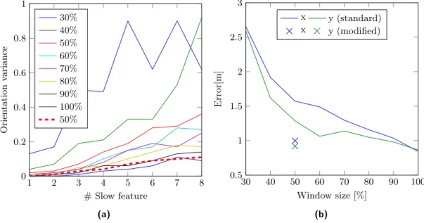
5.1.3 The Impact of the Window Size . . . 37
5.1.4 Discussion . . . 39
5.2 Comparison to Visual Simultaneous Localization and Mapping Methods . 40 5.2.1 Image Acquisition and Preprocessing . . . 41
5.2.2 Experiments in an Indoor Environment . . . 42
viii Contents
5.2.3 Experiments in an Outdoor Environment . . . 48
5.2.4 Discussion . . . 50
5.3 Odometry Integration . . . 52
5.3.1 Unsupervised Metric Learning . . . 53
5.3.2 Fusion of SFA Estimates and Odometry in a Probabilistic Filter . 60 5.3.3 Discussion . . . 61
5.4 Landmark Based SFA-localization . . . 62
5.4.1 Experiments . . . 63
5.4.2 Discussion . . . 69
5.5 Conclusion . . . 70
6 Robust Environmental Representations 73 6.1 Robustness of Local Visual Features . . . 75
6.1.1 Evaluation of the Long-term Robustness . . . 76
6.1.2 Long-term Robustness Prediction . . . 79
6.2 Learning Robust Representations with SFA . . . 87
6.2.1 Learning Short-term Invariant Representations . . . 88
6.2.2 Learning Long-term Invariant Representations . . . 95
6.3 Conclusion . . . 100
7 Navigation Using Slow Feature Gradients 103 7.1 Navigation with Slow Feature Gradients . . . 104
7.1.1 Implementation . . . 105
7.1.2 Experiments . . . 105
7.1.3 Discussion . . . 110
7.2 Future Perspectives for Navigation in Slow Feature Space . . . 111
7.2.1 Navigation with Weighted Slow Feature Representations . . . 112
7.2.2 Implicit Optimization of Traveling Time . . . 115
7.3 Conclusion . . . 117
8 Summary and Conclusion 121
List of Tables
5.1 Network parameters for the simulator experiment. . . 33
5.2 Network parameters for the outdoor experiment. . . 35
5.3 Network parameters for the real world experiments . . . 42
5.4 Localization accuracies for indoor experiment I . . . 45
5.5 Localization accuracies for indoor experiment II . . . 47
5.6 Localization accuracies for the outdoor experiment . . . 51
List of Figures
3.1 Optimization problem solved by SFA . . . 21
3.2 Simulated rotation . . . 24
3.3 Model architecture . . . 25
4.1 Illustration of the marker detection and pose estimation process . . . 29
4.2 Robot platform used in the experiments . . . 30
5.1 Simulator environment . . . 32
5.2 Results for the simulated environment . . . 33
5.3 Training and test error for a varying number of slow feature outputs . . . 34
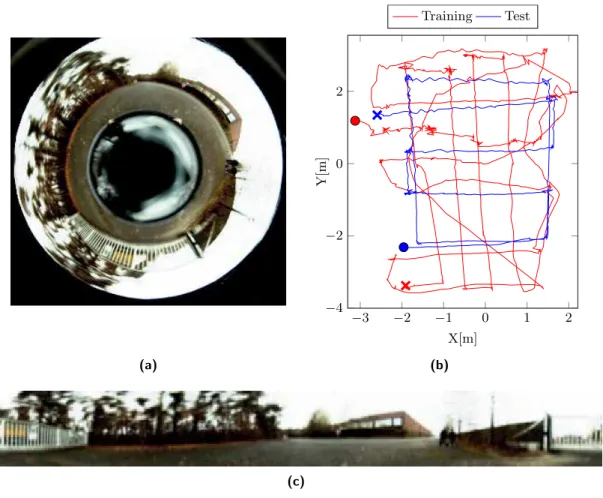
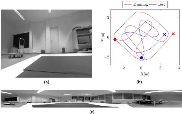
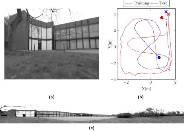
5.4 Example images and trajectories of the experiment . . . 35
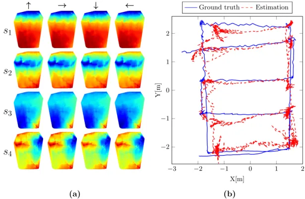
5.5 Results for the real world environment . . . 36
5.6 Training and test error for a varying number of slow feature outputs . . . 37
5.7 Simulated rotation with varying window sizes . . . 38
5.8 Effect of different window sizes . . . 39
5.9 Example images from the perspective camera . . . 43
5.10 Experiment in the indoor environment . . . 44
5.11 Spatial firing maps of indoor experiment I . . . 45
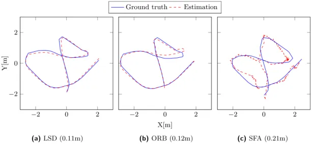
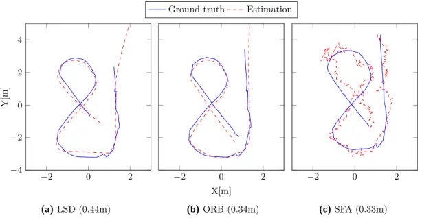
5.12 Estimated trajectories of the best runs in experiment I . . . 46
5.13 Training- and test-trajectory experiment II . . . 47
5.14 Spatial firing maps . . . 48
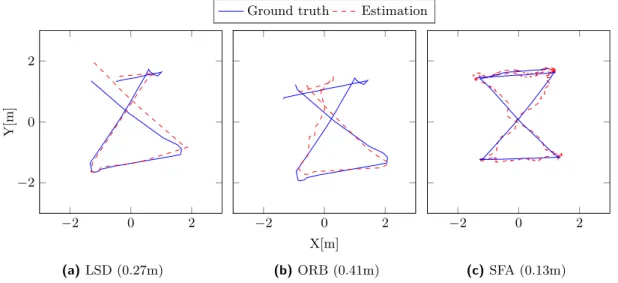
5.15 Estimated trajectories of the best runs . . . 48
5.16 Experiment in the outdoor Environment . . . 49
5.17 Spatial firing maps . . . 50
5.18 Estimated trajectories of the best runs . . . 51
5.19 Illustration of the optimization process . . . 56
5.20 Comparison of supervised and unsupervised regression for the training data 57 5.21 Comparison of supervised and unsupervised regression for the test data . 58 5.22 Comparison of supervised and unsupervised regression for the training data 59 5.23 Comparison of supervised and unsupervised regression for the test data . 60 5.24 Fusion of SFA estimates and odometry using an EKF . . . 62
5.25 Extraction of the marker views . . . 64
xii List of Figures
5.26 Marker visibility for the train and test run . . . 65
5.27 Localization results for single markers . . . 66
5.28 Localization result for two markers . . . 67
5.29 Marker visibility for the training and test run with occlusions . . . 68
5.30 Localization results for single markers with occlusions . . . 69
5.31 Localization results for two markers with occlusions . . . 70
6.1 Garden time-lapse . . . 76
6.2 Results of the feature evaluation . . . 78
6.3 Most stable and unstable features . . . 79
6.5 Illustration of the training process . . . 83
6.6 Matching from summer to spring . . . 84
6.7 Matching features from autumn to spring . . . 85
6.8 Most stable and unstable features . . . 86
6.9 Training- and Test-trajectories and loop closures . . . 90
6.10 Results in the static environment . . . 91
6.11 Changing light . . . 91
6.12 Results with changing light . . . 92
6.13 Dynamic object . . . 93
6.14 Results with a dynamic object . . . 93
6.15 Results with changing light using feedback from BoW loop closures . . . . 95
6.16 Illustration of the training sequence generation . . . 96
6.17 Simulated change in lighting condition . . . 97
6.18 Localization performance for an increasing number of training sets . . . . 98
6.19 Example images for different environmental conditions . . . 99
6.20 Localization performance for an increasing number of training sets . . . . 100
7.1 Simulator environment for the open field navigation experiment . . . 106
7.2 Training trajectory and spatial firing maps for the open field experiment . 108 7.3 Resulting trajectories in the open field experiment . . . 108
7.4 Simulator environment for the navigation experiment with an obstacle . . 109
7.5 Training trajectory and spatial firing maps experiment with an obstacle . 110 7.6 Resulting trajectories for navigation experiment with an obstacle . . . 111
7.7 Spatial firing maps and cost surfaces . . . 113
7.8 Navigation results for an increasing number of SFA-outputs . . . 114
7.9 Navigation with different velocities in the left and right half . . . 117
1 Introduction
Nowadays, there already exist domestic service robots that perform repetitive or unpleas-ant tasks to support us in our daily lives. Vacuum cleaning and lawn mowing robots have been one of the first autonomous robots available as consumer products. Although they are enjoying a growing popularity, their current capabilities are still rather limited. The employed navigation strategies are often constrained to movements along random line segments combined with reactive collision avoidance and some functionality to return to the charging station. To implement a more intelligent navigation behavior a mobile robot needs to create an internal representation or a map from a previously unknown environment in order to determine its own position and plan efficient and viable trajecto-ries. The problems of building a map, localizing within this map as well as planning and executing a path to a target location are fundamental to many robotic application sce-narios. This has raised great research interest in technologies that enable a mobile device to precisely navigate in unconstrained environments. Techniques based on the Global Positioning System (GPS) or laser-range finders have been well established. However, the limited accuracy and availability of GPS and the high cost of laser-range finders prevent their use in domestic service robots produced for the mass market. Cameras on the other hand are cheap, small and passive sensors that offer rich information about the environment and thus provide an interesting alternative. A number of vacuum cleaning robots are already equipped with a camera (e.g. Dyson 360 Eye, Samsung Hauzen) and implement more advanced navigation strategies in the constrained indoor scenario using visual information from the static room ceiling [60]. Research in the field of vision based outdoor navigation is steadily progressing as well and recent work has shown impressive results in mapping large scale environments (e.g. [22, 136, 80, 35, 109]). However, long-term operation in unconstrained outdoor environments is still not robustly solved due to the challenges of visual perception such as changing lighting or weather conditions, different day times or seasons and structural scene changes that strongly influence the visual appearance of a place.
Compared to current technical systems many animals have excellent navigation capa-bilities and are able to quickly and robustly find their way to a food source or their nest. In the brain of rodents spatial information is encoded by different cell types in the hippocampal formation. Place cells fire whenever the animal is within a specific part
2 1. Introduction
of the environment and are mostly insensitive to the orientation of the animal [120]. Head-direction cells, on the other hand, are active when the animal is facing in a certain direction and are invariant w.r.t. its position [154]. Both cell types have been shown to be strongly driven by visual input [59]. The brain is able to extract high level infor-mation, like the own position and orientation in the environment, from the raw visual signals received by the retina. While the sensory signals of single receptors may change very rapidly, e.g. even by slight eye movement, the embedded high level information typically changes on a much lower timescale. This observation has led to the concept of slowness learning [41, 143, 162, 73]. It has already been demonstrated in recent work that a hierarchical network consisting of unsupervised Slow Feature Analysis (SFA) [162] nodes can model the firing behavior of either place cells or head-direction cells from the visual input of a virtual rat only [42]. A theoretical analysis of the biomorphic model in [42] has shown that in slowness learning, the resulting representation strongly de-pends on the movement statistics of the animal. Position encoding with invariance to head direction requires a relatively large amount of head rotation around the yaw axis compared to translational movement during mapping of the environment. While such movement may be realistic for a rodent exploring its environment, it is inefficient for a robot with a fixed camera.
The goal of this thesis is the extension and further investigation of the biologically moti-vated SFA model in order to derive methods for self-localization, the creation of robust environmental representations and navigation that can be applied in outdoor open field scenarios on a real mobile robot.
1.1 Contributions and Outline
This thesis employs the biologically motivated SFA model for spatial representation learning as a basis to address three fundamental problems a mobile robot has to solve in order to autonomously plan and execute tasks within its environment: the ability to perform self-localization, the creation of robust environment representations and the navigation to a specific target location.
Chapter 2 gives an overview of related work which is concerned with solving these prob-lems using vision as the only sensory input.
Chapter 3 details the biologically motivated SFA model that is used to learn a represen-tation of the environment directly from the visual input of a mobile robot. It is based on unsupervised slowness learning and encodes the position of the robot as slowly varying features. The intuition behind slowness learning as well as the concrete algorithm Slow Feature Analysis (SFA) are presented first. Afterwards, the SFA model for spatial cell learning from [42] is introduced. We present an extension to this model allowing to learn orientation invariant representations of the position without requiring a large amount of physical rotational movement. The last section describes the methods for analyzing the
1.1. Contributions and Outline 3
learned slow feature representations.
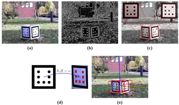
The procedures for generating and capturing the data for the simulator and real world experiments are described in chapter 4. To perform a quantitative metric evaluation the knowledge of the robot’s true position within the environment is required. Since this ground truth information is not directly available in real world settings it has to be acquired by an external system. In the last section of this chapter, we describe a method for ground truth data acquisition based on optical marker detection.
In chapter 5, the spatial accuracy of the learned slow feature representation is analyzed in various simulator and real world self-localization experiments and compared to state-of-the-art vision based methods. Furthermore, we present an unsupervised learning approach to obtain a mapping from slow feature to metric space. The learned map-ping enables the integration of odometry information into the self-localization process to further improve performance. In the last section, an alternative approach for learning spatial SFA representations from single and multiple tracked landmark views is pre-sented.
The problem of creating robust environmental representations enabling a mobile robot to reliably localize itself in changing outdoor scenarios using visual input from a cam-era only is tackled in chapter 6. First, we investigate the long-term robustness of local visual features computed for distinct image patches. These features are commonly used in the context of localization and mapping and could also serve to create alternative im-age representations for training the SFA model. Based on these findings, we propose a generic approach to improve long-term mapping and localization robustness by learning a selection criterion for long-term stable visual features which can be integrated into the standard feature processing pipeline. As an alternative, we introduce a unified approach towards long-term robustness that is solely based on SFA. It takes advantage of the invariance learning capabilities of SFA by restructuring the temporal order of the train-ing sequence in order to promote robustness w.r.t. short- and long-term environmental effects.
In chapter 7, we propose a straightforward approach for efficient navigation in slow fea-ture space using gradient descent. A navigation direction can be inferred from distance measurements between the slow feature values at the current and the target location. It is experimentally shown that the learned slow feature representations enable a reliable and efficient navigation and implicitly encode information about obstacles which are reflected in the SFA gradients. Thus, complex navigation tasks can be solved without explicit trajectory or obstacle avoidance planning. Furthermore, we present preliminary results on an extension to the proposed navigation method for improving robustness in real world applications scenarios and empirically investigate interesting properties of the slow feature representations leading to surprising navigation behaviors.
4 1. Introduction
1.2 Publications in the Context of this Thesis
• M. Franzius, B. Metka, and U. Bauer-Wersing. Unsupervised Learning of Metric Representations with Slow Features. Submitted to the International Conference on Intelligent Robots and Systems (IROS), 2018.
• B. Metka, M. Franzius, and U. Bauer-Wersing. Bio-inspired visual self-localization in real world scenarios using slow feature analysis. PLOS ONE, 13(9):1-18, 2018.
• B. Metka, M. Franzius, and U. Bauer-Wersing. Efficient Navigation Using Slow Feature Gradients. In Proceedings of the 30th IEEE/RSJ International Conference on Intelligent Robots and Systems (IROS), pages 1311-1316, Vancouver, Canada, 2017.
• M. Haris, B. Metka, M. Franzius, and U. Bauer-Wersing. Condition Invariant Visual Localization Using Slow Feature Analysis. In Machine Learning Reports 03/2017, pages 7-8, 2017.
• B. Metka, M. Franzius, and U. Bauer-Wersing. Improving Robustness of Slow Feature Analysis Based Localization Using Loop Closure Events. In Proceedings of the 25th International Conference on Artificial Neural Networks (ICANN), pages 489-496, Barcelona, Spain, 2016.
• B. Metka, A. Besetzny, U. Bauer-Wersing, and M. Franzius. Predicting the Long-Term Robustness of Visual Features. In Proceedings of the 17th International Conference on Advanced Robotics (ICAR), pages 465-470, Istanbul, Turkey, 2015. • B. Metka, M. Franzius, and U. Bauer-Wersing. Outdoor Self-Localization of a Mobile Robot Using Slow Feature Analysis. In Proceedings of the 20th International Conference on Neural Information Processing (ICONIP), pages 249-256, Daegu, South Korea, 2013.
2 Localization, Mapping and Navigation
This chapter serves as an overview of the main methods enabling autonomously navi-gating mobile robots using vision as the only sensory input. In order to determine its own location within the environment a robot needs an internal representation of the environment. However, the construction of such a map from sensor measurements in turn requires knowledge of the precise position. Therefore, the problem of localization and mapping is usually solved simultaneously in an incremental fashion. The next sec-tion briefly introduces established approaches for simultaneous localizasec-tion and mapping (SLAM) but also reviews methods trying to mimic biological models and the recently emerging methods based on deep learning. Changes in the environment caused by differ-ent lighting conditions, seasons or structural scene changes induce high variability into the appearance of a place and thus pose a severe challenge for vision based localization and mapping methods. Section 2.2 gives an overview of a variety of approaches aiming at robust long-term operation. The ability to create a map and to determine the own position are the prerequisites enabling a mobile robot to perform the high-level task of navigation. Navigation methods based on different environment representations are reviewed in section 2.3.
2.1 Localization and Mapping
The ability to build a map of the environment and to determine the own location within the acquired map is a prerequisite for autonomously acting mobile robots. While lo-calization and mapping can be performed with different kinds of sensors, vision based approaches are especially appealing because of the low cost, weight and the high avail-ability of cameras. Research in the field is steadily progressing and recent work has shown impressive results in mapping large scale environments (e.g. [22, 136, 80, 35, 109]). Most vision based approaches extract local visual features from the captured images to esti-mate the motion of the camera and create a sparse 3D representation of the environment. The first step in feature extraction is the identification of accurately localizable and dis-tinguishable interest points in the image like corners [53, 140, 130] or blobs [92, 86, 10]. Afterwards, a descriptor is created from the surrounding image patch using gradient information [86, 97, 10] or pixel-wise intensity comparisons [17, 131, 82, 2].
6 2. Localization, Mapping and Navigation
spondences between features from the current image and stored map features can be established by a nearest neighbor search in descriptor space. This process is called fea-ture matching.
Determining the own position within the environment requires some kind of internal representation or map. In its simplest form, such a representation consists of a database of images collected for a distinctive set of places. Localization can then be solved by a search for the database image which is closest to the image of the current location. To perform the matching efficiently the images are usually transformed to a lower dimen-sional representation, e.g. by extracting local visual features and storing them in a tree structure [135]. In topological maps the place representations are stored in nodes that are linked to neighboring places, which adds knowledge about the connectivity between places [23, 22, 102, 95]. The current estimate of the own position is a strong prior which allows to reduce the search space and consequently improves accuracy. Adding spatial information from ego motion estimates to the links between places allows to reconstruct the spatial layout of the environment and enhances navigation capabilities [3, 100]. The ability to recognize previously seen places, known as loop closure detection, is also re-quired in other mapping systems as a means to re-localize after tracking failures or in the absence of sensor measurements. Loop closures allow to correct the current pose estimate and to reduce the uncertainty. An extensive overview of place recognition and topological mapping is given in [88].
Estimating the ego motion of a camera from a sequence of images is known as visual odometry [117]. Initially, the camera motion between two frames is recovered from the essential matrix which can be estimated from five feature correspondences [116]. Given the relative camera motion and the two image projections of a point, the 3D position of the point can be reconstructed by triangulation [55]. Subsequently, the camera motion is obtained from 3D-2D correspondences and the application of nonlinear optimization techniques which minimize the re-projection error. The quality of the estimated trajec-tory can be improved by jointly optimizing the pose of the camera as well as the sparse 3D scene structure applying bundle adjustment [157] over a local window of past frames. An extensive tutorial on feature based visual odometry is presented in [133, 45]. Another approach for camera motion estimation and 3D scene reconstruction is based on direct image alignment using dense information from all [115] or semi-dense information from high gradient pixels [36]. Based on the recent image and its corresponding inverse depth map the pose of the camera is estimated by finding the motion parameters generating a synthetic view that minimizes the photometric error w.r.t. the current image. Using monocular vision only, the scale of the estimated camera motion and scene depth is an arbitrary factor. The absolute scale can be recovered using additional sensors [118], knowledge about the size of a reference object [26] or the height of the camera when moving on the ground plane [141].
2.1. Localization and Mapping 7
the own position will inevitably diverge from the real one since small errors accumulate over time. This drift can only be corrected by relating current sensor measurements to a previously constructed map. By detecting a loop closure the deviation of the current estimate from the past one can be corrected and back-propagated along the trajectory. In addition to pose drift, monocular approaches also need to account for a drift in scale which is tackled in [147] by using similarity transformations to represent camera motion. The problem of incrementally building a map of the environment and at the same time determining the own position within this map is known as simultaneous localization and mapping (SLAM). To solve the SLAM problem there exist mainly three paradigms that will be briefly discussed in the following.
Extended Kalman Filter The work by Smith et al. [139] introduced the Extended Kalman Filter (EKF) formulation of the SLAM problem. The core principle is to rep-resent the pose of the camera and the positions of map features as a joint probability distribution with a single state vector and a corresponding covariance matrix reflecting the uncertainties. Based on the current estimate the next pose is predicted using a motion model and the expected position of the map features is computed. Associating the measured features to the map features enables a correction of the estimate. The Kalman equations require a linear motion and measurement model in order to maintain a Gaussian distribution. This is achieved by linearizing the involved functions around the current mean. The first real-time capable monocular EKF-SLAM system was presented by Davison et al. [25, 26]. They estimated the full 3D pose of a hand-waved camera and 3D feature locations in an indoor environment assuming a constant velocity model. Since the complexity of updating the covariance matrix is quadratic in the number of features, the map size is limited to a few hundred features in practice. The authors of [20] employed a sub-mapping strategy to enable the application in larger scale outdoor en-vironments. Estimating the depth of a feature requires at least two measurements from different viewpoints. In [26] feature initialization is delayed until the depth uncertainty is small enough. The authors of [107] instead used an inverse depth parametrization which allows to directly integrate new features so that they immediately contribute to improving the estimate. Despite its successful application in real-time visual SLAM there remain some issues with the EKF approach. Besides the computational scaling it can not represent a multi-modal distribution of the current state caused by ambiguous measurements. Falsely established data associations lead to a divergence of the estimate that can not be corrected afterwards. Furthermore, the required linearization introduces errors in the estimate.
Particle Filter A Rao-Blackwellized particle filter solution to the SLAM problem was first introduced in [105] and later improved in a follow up work [106]. The approach maintains a set of particles where each particle represents an estimate of the trajectory
8 2. Localization, Mapping and Navigation
together with its own feature map. The map features of a single particle are represented by low dimensional EKFs, exploiting the fact that the positions of map features are conditionally independent given the trajectory. The complexity is logarithmic in the number of features, enabling the creation of maps containing thousands of features. In contrast to the EKF approach it is possible to accurately represent the state estimate as a multi-modal distribution. The process starts with the generation of random particles. A motion model is applied in order to predict the next position of the robot and the expected position of map features. After a data association step the map is updated and the agreement of predicted and measured feature positions is used to assign an importance weight to each particle. In the subsequent re-sampling step the importance weights are used to remove unlikely samples and to replace them by new ones. While the original work used range sensors, the particle filter approach was also successfully applied using monocular [32] and stereo cameras [137]. One problem is the determination of the particle set size, that is needed to accurately map a certain environment and to maintain a sufficiently diverse set over long trajectories.
Graph Optimization Most modern approaches formulate SLAM as a problem of pose-graph optimization [16]. The nodes in the pose-graph correspond to camera poses or feature locations that are connected via edges representing spatial measurements from odometry and feature observations. The constructed graph is processed using nonlinear optimiza-tion (bundle adjustment) to find the spatial configuraoptimiza-tion of nodes that minimizes the measurement error. Although the graph formulation was first introduced in 1997 [89], it has only become popular in recent years with the introduction of efficient and robust techniques (e.g. [28, 52, 121]) and the publication of generic graph optimization frame-works (e.g. [1, 76, 63]). Klein and Murray [70] presented their Parallel Tracking and Mapping (PTAM) approach, a real-time capable Monocular SLAM system. They per-form feature and pose tracking in one thread while the map optimization is perper-formed on a subset of carefully selected keyframes in the background. Strasdat et al. [147] pre-sented a keyframe-based method using similarity instead of rigid body transformations to deal with the inherent problem of scale drift in monocular SLAM. In [146, 148] they concluded that the performance of graph optimization methods is superior to probabilis-tic filtering approaches (EKF, parprobabilis-ticle filter) when the number of features is increased. Recently, the feature-based ORB-SLAM [109] and the semi-dense LSD-SLAM [35] have been demonstrated to enable precise localization and mapping in large scale environ-ments using a single camera and running in real-time on the CPU.
A detailed introduction into probabilistic filtering for SLAM can be found in the tu-torials from Durrant-Whyte and Bailey [31, 7] and the book from Thrun et al. [155]. A tutorial on graph-based SLAM can be found in [51]. A survey of visual SLAM methods is presented in [46]. The current state of the art and open challenges are discussed in [16].
2.1. Localization and Mapping 9
Biologically Inspired Models Many animals have excellent localization and navigation capabilities and seem to be able to easily find their way to a food source or nest lo-cation even in difficult environmental conditions. Ants are assumed to combine path integration and image matching where the current scene view is compared to stored snapshots from specific locations in order to navigate in their natural habitat [160, 21]. In [77] the authors implemented a model of ant navigation on a real robot in a desert environment with artificial landmarks. Path integration is based on wheel odometry and global heading direction obtained from a polarized-light compass system. The compass direction was used to align the perceived panoramic view from the current location to the stored snapshot at a target location. Navigation was then performed by computing a homing vector based on the image matching. Due to their dichromatic vision with peak sensitivities in the ultraviolet and green range the authors of [124] suggest that ants might extract and store skyline information, i.e. the border between sky and none-sky regions to determine a homing direction. In [144] the authors present results from topo-logical localization using binary images encoding sky/non-sky pixels as a representation for places along a 2km route.
In 1971 O’Keefe and Dostrovsky discovered the existence of place cells in the hippocam-pus of rats whose activity is highly correlated with the animal’s location in the environ-ment [120]. Several years later, neurons encoding the orientation of the rat, so called head-direction cells, have also been identified [154]. A computational model of place and head-direction cells was presented in [5]. Visual cues and path integration were combined in a Hebbian learning framework to create a population of place cells enabling a small robot to navigate within a 60×60 cm area with bar-coded walls. A similar approach was presented in [9] where individual places and their spatial relations were encoded in a topological map. The model was also able to learn and unlearn navigation actions towards specific goal locations. Experiments have been performed in an eight-arm radial maze and a single and double T-Maze with artificial visual cues on the walls.
The focus of the aforementioned models is rather on producing plausible animal naviga-tion behavior than performance in robotic scenarios. However, another approach inspired from rat navigation, called RatSLAM [101], is also concerned with real world applica-tion scenarios. The pose is encoded by an activity packet in a 3D continuous attractor network with axes representing (x, y, ϕ), i.e. the pose of the robot. Self-motion cues and visual template matching inject energy into the network shifting the peak of activity. To enable the mapping of larger environments the model was extended by organizing unique combinations of local views and pose codes in a topological experience map. The map is optimized after loop closures using graph relaxation and enables the model to maintain a consistent spatial representation over extended periods of time. In [99] a 66 kilometer urban road network was successfully mapped with a single webcam.
A comparison of mapping and navigation principles from biology and robotics is given in [98].
10 2. Localization, Mapping and Navigation
Deep Learning The technological and methodical progress in recent years enabled the training of deep convolutional neural networks (CNNs) and led to major advance-ments in many fields of computer vision e.g. image classification [74, 56], object detec-tion [128, 129] and image segmentadetec-tion [50, 85]. The well established SLAM methods are focused on multiple view geometry as well as on probabilistic methods and optimiza-tion techniques. However, since SLAM systems are highly modular researchers tried to solve different parts of the SLAM pipeline using CNNs. In [29] the authors used a small CNN to extract image patch descriptors that are superior to handcrafted ones like SIFT [86] and SURF [10] in image classification tasks. The training data was generated by randomly sampling 32×32 patches and applying a family of transformations like translations, rotations and color adjustments. The set of transformed patch variants was declared as one class and the network was trained to discriminate between classes. The problem of feature matching, i.e. identifying the same patch across images, was approached in [163] by learning a similarity function with a CNN. Multiple architectures were trained with tuples of image patches representing either the same patch extracted from different images or dissimilar ones. In several feature matching experiments the best results were achieved using a two-channel architecture where the two patches are processed as a single image made of two channels. A model for joint end-to-end learning of dense scene depth and ego-motion from monocular images was presented in [168]. The synthesis of new views based on the scene depth and ego-motion is the basis of jointly training two CNNs for each task. The depth prediction network processes a single im-age and assigns a depth value to each pixel. The ego-motion network takes as input a sequence of images and outputs the Euler angles and translation vectors from each source view to a reference view. The depth and ego-motion estimates are then used to synthesize the subsequent view. The loss is defined as the sum of absolute differences between the pixel intensities of the real and the synthesized view. Evaluations on depth and ego-motion benchmarks demonstrated a performance comparable to state of the art methods. The authors of [153] integrated a CNN for pixel-wise depth prediction into a dense SLAM system. The predicted depth was fused with the depth values estimated by the SLAM system to improve accuracy in low texture/gradient image regions and under pure rotational movement which prevents geometric depth estimation due to the lack of a stereo baseline. A complete model for end-to-end regression from monocu-lar images to camera poses coined Pose-Net was proposed in [68]. A CNN network pre-trained on a large scale image classification task is used to regress the 3D position and orientation of camera in previously explored scenes. The ground truth is generated using a feature based structure from motion (SfM) approach which is similar to SLAM approaches relying on pose-graph graph optimization previously introduced in this chap-ter. The network output is a 7-dimensional vector representing the 3D position and the orientation encoded as quaternion. The loss is defined as the Euclidean norm between the predicted and the ground truth pose with an additional scaling term to balance
2.2. Long-term Robustness 11
the influence of position and orientation errors. The localization error in the presented experiments is higher compared to feature based localization w.r.t. to the point cloud created from SfM. However, due to the large data set used for pre-training, the obtained convolutional features enabled localization under a range of varying appearances, e.g. daytime or weather, where the feature based approaches failed. In a follow up work [67], the authors extended their model by a fine-tuning step using a geometric loss function defined by the re-projection error of 3D scene points given the estimated pose. Although the localization accuracy improved over the base model it is still worse than a feature based approach. Currently end-to-end learning for camera localization does not achieve state-of-the-art performance. However, it is superior in terms of robustness w.r.t. ap-pearance changes of the environment. A further advantage of the CNN pose regression is the fixed model size and interference time which are both independent from the size of the mapped environment. Considering the decades of research invested into SLAM algorithms and the recent emergence of end-to-end deep learning approaches, we will probably see further advancements in the future. In the short term, some of the stages in the classic SLAM pipeline might be replaced by learning methods.
2.2 Long-term Robustness
Appearance changes of the environment induce high visual diversity into images of the same place visited at different times. This poses a severe challenge for vision based localization and mapping methods. Therefore, different approaches towards long-term autonomy have been proposed recently.
Dynamic Maps Over time the appearance of the environment might undergo substan-tial changes in appearance so that a previously constructed map becomes obsolete. If the current sensor measurements are no longer coherent with the stored map data, local-ization will inevitably fail. In order to reflect changes in the environment the map can be updated by removing data which does no longer conform to the current environmental condition and adding new measurements. Instead of updating the sensor representation of a place, a map might also include multiple representations of the same place in differ-ent conditions. In [27] the authors create a topological map of the environmdiffer-ent where each node represents a specific place together with a descriptor obtained from the corre-sponding sensor measurements. The descriptors are SURF-features [10] extracted from the images. A short-term and long-term memory structure is employed to deal with tem-porarily and structural changes in an indoor environment. Stable features are gradually moved from short-term to long-term memory to adapt the map to a changing environ-ment. The capacity of the long-term memory is constrained by a forgetting mechanism which removes unused features. In a nine week indoor experiment an improvement was shown compared to using a static map representation. Selecting the right parameters for
12 2. Localization, Mapping and Navigation
updating the long-term memory depends on the dynamics of the environment in order to find the right balance between stability and plasticity. Dynamic changes in indoor environments are addressed in [72]. The authors present a system based on stereo visual odometry and visual feature based place recognition to create multiple representations of the environment over time. The map is represented as a pose graph of keyframes where the nodes contain a feature representation which is used by the place recognition module. In case of odometry failures and for global localization the current sub-map is linked with a high uncertainty to the existing map. If the place recognition system detects a loop closure, the sub-map is linked to the existing map and the initial ’weak link’ is removed. The update and deletion of nodes is designed to preserve diversity while at the same time limiting the maximum number of nodes. Since the approach relies on visual features for place recognition, the maintenance of a consistent map is only possible under slight appearance changes. A similar approach of Churchill et al. [19] is to build and maintain dynamic maps of the environment where the diversity in the appearance of the environment is captured by different visual experiences. A visual experience is a sequence of estimated poses and the corresponding visual features obtained with a stereo visual odometry system. Multiple localizer running in parallel try to match the current frame to existing experiences. In case the system fails to localize a new experience is created. The authors demonstrate localization and mapping in an outdoor environment at different day times and changing weather conditions over the course of three month. Since the approach requires the successful localization in previous experiences in order to link the current one to the existing map, it can only deal with gradual changes. Milford et al. presented an extension to their RatSLAM model to enable long-term navigation in a dynamic indoor environment over the course of two weeks [100]. The unique combina-tions of local views and pose codes from the continuous attractor network are defined as experiences which are organized in a graph like map that enables the model to maintain a consistent spatial representation over extended periods of time. Graph relaxation is used to correct the map after loop closure detections. If the robot visits a new place or the appearance a known place has changed a new experience is created. To prevent the map from growing indefinitely nodes from regions with a high density of experiences are deleted randomly.
Robust Representations Instead of adapting the map to changes in the environment another approach towards long-term autonomy is to transform the sensor measurements to robust or invariant representation which are less affected by appearance variations. Considering short timescales, changes in illumination are one of the main causes for the failure of a vision based localization system. Lighting invariance is tackled by sev-eral authors at different levels of the image processing pipeline. In [165] the exposure time of a camera is optimized using a gradient-based image quality metric which ex-ploits the cameras’ photometric response function. The authors demonstrate a superior
2.2. Long-term Robustness 13
performance in visual odometry tasks compared to the camera’s built in auto-exposure control. In [93] the effects of shadows are mitigated by a transformation of the images to a shadow invariant representation where the pixel values are a function of the underlying material property. Mapping and localization is then performed in parallel with standard gray-scale and illumination invariant images.
Local visual features are broadly used in the context of visual SLAM. To some extent they are robust w.r.t. lighting, viewpoint and scale changes. However, due to illumina-tion effects, cast shadows and dynamic objects visual features extracted from a reference frame can usually only be matched within a limited period of time and the number of true positive matches might decrease drastically even after a few hours [125]. The authors of [158] investigated the suitability of SIFT and SURF features for coarse topological image based localization in a long-term outdoor scenario. Their results from a nine month experiment have shown that a reliable localization is not possible using descrip-tor matching alone. Through the application of the epipolar constraint, which takes the geometric relation between matched features into account, they could reduce the number of false positives and achieved a successful localization in 85%-90% of the trials [159]. The authors of [65] improve the robustness of topological localization using visual word occurrences by only considering features that can be persistently tracked over several frames and storing their average. In [62] a certain track is traversed several times under different conditions while keeping track of feature occurrences per place. The statistics collected during the training runs allow to model the probability of feature visibility per place.
Some authors proposed learning approaches to obtain illumination invariant feature descriptors. In [18] features are tracked over a sequence of images from a time-lapse video featuring dynamic lighting conditions. Matching and non-matching pairs of image patches are discriminated by a contrastive cost function. Genetic optimization was used in [78, 79] to obtain an illumination invariant descriptor from a pool of elementary de-scriptor building blocks. Although the authors demonstrate superior performance with respect to standard feature matching, illumination invariance addresses only a part of possible appearance changes.
Instead of focusing on small image structures like corners, blobs or edges the authors of [94] propose to learn place specific detectors for broader image regions which likely correspond to physical objects like windows, trees or traffic signs. Provided with several images of the same place in different conditions they train a number of linear Support Vecor Machines (SVMs) per place to robustly detect distinctive elements in the scene. Odometry information between nodes in a topological map is used as a selection prior in order to choose the place specific SVMs. The authors demonstrate successful coarse metric localization under challenging appearance variations. However, their approach requires to select images of the same place from different runs for training the SVMs which might be hard to accomplish in the first place.
14 2. Localization, Mapping and Navigation
Approaches using features from a pre-trained deep Convolutional Neural Network (CNN) for robust place recognition have been proposed by several authors. S¨underhauf et al. [149] investigated the effectiveness of CNN features extracted from different layers of AlexNet [74]. They concluded that features from the third convolutional layer are highly robust w.r.t. appearance changes while features from higher layers are less depen-dent on the viewpoint. Using the CNN features as holistic image descriptor improved the place recognition performance over existing methods based on conventional visual features and sequence matching. Depending on the specific data set, either a network trained especially for semantic scene recognition [167] or a network trained for generic object recognition [74] performed best. In [150] they extended the approach to achieve condition and viewpoint invariance using CNN descriptors computed for distinctive im-age regions obtained by an object proposal method [169]. In [4] the authors propose a method which integrates a trainable Vector of Locally Aggregated Descriptors (VLAD) layer into a CNN. The VLAD vector aggregates the distances of quantized features to their nearest visual word from a code book. The network is trained with a ranking loss function on Google Street View Time Machine where images of the same place in different conditions can be obtained. The output of the VLAD layer is used as image descriptor and the place recognition is performed by a nearest neighbor search. The methods based on CNN features were proven to enable place recognition under challeng-ing conditions providchalleng-ing coarse metric localization. However, the proposed methods have high demands for computational and memory resources which renders them unsuitable for the application on small mobile platforms.
Image Sequence Matching Milford et al. [102] demonstrated localization along one dimensional routes across difficult conditions with severe changes in appearance. The approach, named SeqSLAM, matches sequences of images rather than finding a sin-gle global best match. Matching is performed directly on the down-sampled, patch-normalized images. The holistic image matching over sequences restricts this approach to one dimensional traversals along a defined route without deviations in lateral posi-tion and assumes a constant velocity. Improvements to this approach were presented in [123]. The robustness is increased by blackening out the sky regions before match-ing the images. Instead of samplmatch-ing at a fixed rate, the samplmatch-ing of images along the trajectory is driven by distance measurements from odometry to deal with variable ve-locities. The tolerance w.r.t. lateral deviations is increased by matching images over a predefined range of offsets. Naseer et al. [112] use a dense grid of Histogram of Oriented Gradients (HOG) [24] as image descriptors. They build a data association graph that relates image sequences retrieved in different seasons and solve the visual place recogni-tion problem by computing network flows in the associarecogni-tion graph. In a follow up work they have demonstrated that the performance improves further when using features from pre-trained CNN as global image descriptors [111]. While the approaches demonstrate
2.3. Navigation 15
robust place recognition under severe appearance changes, the sequence matching and the assumption of similar viewpoints renders them impractical for localization in open field scenarios.
Appearance Change Prediction A place might look very different when it is observed in different conditions, e.g. when comparing its appearance in the morning and the afternoon or in summer and winter. Hence, when using global image descriptors for image comparison in different conditions the distance in descriptor space might become prohibitively large. Instead of directly matching images from different conditions some authors proposed to learn a mapping that allows to translate the appearance of a place from one condition to another. In [113, 114] the authors create a common vocabulary of corresponding visual words from aligned image streams captured in different seasons along the same route. The images from the current condition are segmented into visual words which are then translated to the target condition using the learned vocabulary. The authors demonstrated that sequence based place recognition (SeqSLAM) benefits from the appearance change prediction. Global illumination changes occurring over the course of a day are tackled in [87]. A linear regression model is trained with image pairs of the same place at different times of the day in order to learn the corresponding transformation. Results from their experiments show that the appearance change predic-tion yields a substantial performance improvement compared to direct image matching between different daytimes. In [84] the authors train coupled Generative Adversarial Networks to translate between images from different seasons. Although the methods have been shown to improve the localization performance, the identification and man-agement of conditions has not been investigated so far.
2.3 Navigation
In order to execute tasks in a spatial environment a mobile robot needs to plan a viable path to a given target location and then execute this plan using appropriate motion com-mands and avoiding collisions with objects. These navigaton strategies have different levels of complexity ranging from reactive motion execution to path planning in metrical maps [96, 13].
Reactive techniques for collision avoidance can be carried out without having an envi-ronmental representation using only the currently available sensor measurements. The authors of [142] demonstrated a method based on optical flow [58], which is defined as the 2D displacement of every pixel between consecutive frames captured with a moving camera, to circumnavigate obstacles. Objects in the field of view create optical flow vectors occupying increasingly larger areas of the image when they are approached by the robot. In order to avoid collisions the magnitude of the optical flow was kept in balance between the left and right half of the image.
16 2. Localization, Mapping and Navigation
Navigation to a target location which is in the direct line of sight is known as visual homing. Since the difference between the image from a given target location and im-ages from nearby locations increases smoothly over space, navigation can be performed by successively estimating the movement direction that minimizes the distance in im-age space [164, 104]. Navigation in larger environments with a restricted viewing area requires a representation containing several snapshots organized in a topological map. In [44] images from distinct places have been stored as nodes in a topological map where the links between nodes represent their adjacency relationships. The planning of a global path was implemented using a graph search algorithm. A visual homing method based on feature correspondences was used to navigate between nodes. A similar approach using omnidirectional vision was presented in [14].
Graph search techniques like A* [54] are also used to plan trajectories in occupancy grid maps where the environment is discretized into equally sized cells with an assigned prob-ability of being occupied by an obstacle. They are usually generated using range sensors like stereo vision [34, 110]. For navigation in grid or topological maps A* is guaranteed to find the optimal path given an admissible distance heuristic. However, it is memory and computationally intensive for large environments with many obstacles. During the path execution deviations caused by sensor measurements have to be detected and cor-rected. If the deviations become too large a re-planning step has to be initiated. Instead of finding a path from the current to a target location one can create a universal plan, which assigns a motion command to every position in the environment leading the robot to a specified target. The authors of [5] created such a universal plan to implement navigation in their biomimetic model of place cells. They assigned a reward to the tar-get location and used reinforcement learning to obtain a policy which selects the motion command with the highest expected reward in response to an input from the place cell network. However, the required additional learning phase with random explorations of the environment might not be feasible in real world application scenarios.
Another approach for navigation in metrical space is the potential field method that is based on gradient descent in a vector force field defined by an attractor at the tar-get position and repulsive forces from obstacles [69, 8]. It is an elegant formulation of the navigation problem, however, a known limitation of the approach are local minima caused by certain types of obstacles or their spatial configuration [156]. By designing an optimal navigation function having a global minimum this problem can be avoided [30]. However, determining such a function is only feasible for small environments with a low complexity [96].
The feature-based maps introduced in a previous section allow to precisely localize a mobile robot and accurately model the sparse scene structure while being memory effi-cient. However, since the absence of a feature does not necessarily imply free space, e.g. a low-textured wall might not be represented in the map, these maps are not optimal in terms of path planning and navigation [46]. A general review of mapping and navigation
2.3. Navigation 17
3 Unsupervised Learning of Spatial
Representations
This chapter introduces a model based on unsupervised slowness learning that enables a mobile robot to extract a spatial representation of the environment directly from the visual input captured during an exploration phase. The resulting representation encodes the position of the robot as a set of slowly varying features that are invariant w.r.t. its specific orientation. The intuition behind the principle of slowness learning is given in section 3.1. Slow Feature Analysis (SFA), the concrete algorithm that is used in this work, is discussed in section 3.2. It has been shown in previous work that a hierarchical, converging SFA network can model the activity of cells in a rat’s brain that form a neural representation of its spatial attributes by directly processing the views from a virtual rat [42]. The model learns either representations of the position or the orientation depending on the movement statistics during the unsupervised learning process. This hierarchical SFA network for spatial cell learning is the basis for this work and is presented in section 3.3. The specific network architecture and a training scheme for learning orientation invariant representations of the position is described in section 3.4. The methods for analyzing the learned slow feature representations are detailed in section 3.5.
3.1 Principle of Slowness Learning
Extracting relevant information from received sensory signals is an important prerequi-site to interact with the environment. When we visually perceive a scene our brain is able to extract a high level representation from the raw visual sensory signals it receives. If an object passes our field of view the stimuli of a single receptor in the retina may change very rapidly, while the high level information (what objects are present, and where are they located) usually changes on a much slower timescale. Since the reconstruction of relevant information from the received signal is not directly coupled to a feedback or supervision signal it is assumed to be guided by statistical regularities in the input data. One of these regularities is the difference in the timescales of the quickly varying stimuli and the slowly varying high level representation. This leads to the assumption that slow-ness is a general learning objective in the brain. If the relevant information is expected
20 3. Unsupervised Learning of Spatial Representations
to change slowly it should be possible to recover it by extracting slowly varying features that are embedded in the raw visual stimuli. The resulting learning principle does not rely on external supervision signals, i.e. it is unsupervised, and thus only depends on the statistics of the training data. Although slowness learning is concerned with identifying slowly varying signals the extraction of these signals needs to be instantaneous in order to adequately react to relevant events.
A well known approach for unsupervised learning is Principal Component Analysis (PCA). It finds a rotated coordinate system such that the dimensions of the data in the new coordinate system are de-correlated. Furthermore, it sorts the eigenvectors, which form the new basis vectors, in descending order according to the corresponding eigenvalues. Hence, PCA is often used for dimensionality reduction by discarding di-mension with low variance. In contrast to unsupervised slowness learning, the temporal order of the data samples is irrelevant to PCA. Therefore, PCA yields the same result for different permutations of the data. However, the temporal structure of the data often contains useful information and one might want to obtain similar outputs for temporally close input samples. Measures of similarity or temporal stability constitute the basis for slowness learning methods [41, 143, 73].
3.2 Slow Feature Analysis
Slow Feature Analysis (SFA) as introduced in [161, 162] is the slowness learning method used in this thesis. SFA solves the learning problem of finding instantaneous scalar input-output functionsgj(x) that transform a multidimensional time seriesx(t), in our
case images along a trajectory, to slowly varying output signals such that the signals sj(t) : =gj(x(t))
minimize
∆(sj) : =hs˙2jit under the constraints
hsjit= 0 (zero mean), hs2jit= 1 (unit variance),
∀i < j :hsisjit= 0 (decorrelation and order)
withh·it and ˙s indicating temporal averaging and the derivative ofs, respectively. The ∆-value is a measure of the temporal slowness of the signalsj(t). It is given by the mean
3.2. Slow Feature Analysis 21 x(t) s(t) =g(x(t)) g(x) t t x1 x2 xN s1 s2 s3
Figure 3.1:Illustration of the optimization problem solved by SFA.SFA finds functions g(x) that transform a time varying multidimensional input signal x(t) to output signalss(t) = g(x(t)) that vary as slow as possible. Once the training is finished slow features are computed instantaneously from a single snapshot of the input signal. Adapted from Figure 1 in http: //www.scholarpedia.org/article/Slow_feature_analysis.
of the signal’s squared temporal derivative, so small ∆-values indicate slowly varying signals. The constraints avoid the trivial constant solution that is maximally slow but carries no information and ensure that different functions g code for different aspects of the input. Furthermore, slow features s are required to be instantaneous outputs of functions g so that slowly varying signals can not be obtained by temporal filtering. The optimization problem solved by SFA is illustrated in Fig. 3.1. If one considers a finite function space, e.g. all polynomials of a degree two, SFA can be implemented by performing the following sequence of steps:
• First, the data is expanded into the non-linear space that is considered for the given problem, e.g. all polynomials of degree two.
• Subtracting the sample mean centers the expanded data points and satisfies the zero mean constraint.
• Applying PCA to the covariance matrix of the expanded and centered data points yields a set of eigenvectors which are the basis of a new coordinate system where the dimensions are de-correlated. The data points are normalized by projecting them on the set of eigenvectors and dividing by the square root of the corresponding eigenvalues.
• The temporal variation is measured on the normalized data points by approximat-ing the temporal derivatives with the differences between consecutive data points. Applying another PCA to the covariance matrix of the temporal derivatives and projecting the data on the axes with the smallest variance yields the slow features.
22 3. Unsupervised Learning of Spatial Representations
The function g(x) is represented by the sequence of all steps. A closed form solution of SFA based on solving a generalized eigenvalue problem was presented in [11]. The implementation of SFA that is used in this work is part of the Modular toolkit for Data Processing (MDP) [170].
SFA originates from the field of computational neuroscience and has been used to model complex cells in the primate visual system [11]. However, it was also applied in a number of technical applications, like human action recognition [166], monocular road segmentation [75] or object recognition and pose estimation [43] to extract invariant features or to obtain low dimensional and meaningful representations from the raw input data.
Since most problems of interest are non-linear the data is usually expanded into the considered function space (e.g. all polynomials of degree 2−3). Due to the non-linear expansion SFA becomes impractical for high dimensional data as the complexity is cubic in the number of dimensions. In order to efficiently process high dimensional data SFA can be applied iteratively in a hierarchical converging network. The input data is partitioned into small blocks which serve as input to distinct SFA nodes in the input layer. Blocks of locally learned SFA-outputs from these nodes are then fed as inputs to the next layer of SFA nodes. A limitation of the number of SFA-outputs that are passed to the next layer and the block-processing reduce the overall dimensionality with every layer. At some point, global SFA becomes feasible with a single node that effectively perceives the whole input data. Although the hierarchical processing does not guarantee to find the globally optimal solution it has been proven to yield feasible results in many practical applications [37].
3.3 Model for the Formation of Place and Head-Direction Cells
Cells in the hippocampus of rodents have been discovered that form a neural represen-tation of the animal’s spatial attributes like its position in space or its head-direction. Place cells fire whenever the animal is in a particular location and are independent from its orientation [120]. Head-direction cells on the other hand are invariant with respect to the spatial position and are only sensitive to the orientation of the animal [154]. Franzius et al. [42] introduced a model consisting of multiple, converging layers of SFA-nodes that is capable of extracting spatial information directly from the raw visual stimuli of a vir-tual rat. The last node in the network performs sparse coding and produces responses similar to those of place and head-direction cells. Experiments were performed in a rectangular simulator environment with textured walls. The model was trained with the 320◦views of the rat that were captured during a random exploration of the environment following Brownian motion with different ratios of translational and rotational veloci-ties. It has been shown that the type of spatial cells that develop only depends on the movement statistics of the virtual rat during the training phase. For low a translational
3.4. Model Architecture and Training 23
speed and quick head movements the resulting SFA-outputs are invariant with respect to the orientation and only code for the position of the rat. Slow head movement and fast translational speed results in functions that are position invariant and code for the head-direction. They also introduced an analytical method to determine the theoreti-cally optimal solutions under the constraints that the environment is kept unchanged for the duration of the experiment. Having knowledge about the spatial configuration of the rat, defined by its position and head-direction (x, y, ϕ), the corresponding view can be determined. The same applies for the views that determine the exact configuration of the rat if the environment is diverse enough. This leads to the simplified problem of performing SFA on the low dimensional configuration space instead of the high di-mensional views. In this case it becomes feasible to compute the optimal solution for SFA analytically. For a rectangular shaped training area the derived optimal output functions encode the position on the coordinate axes and the orientation of the robot as standing cosine-/sine waves.
3.4 Model Architecture and Training
3.4.1 Orientation Invariance
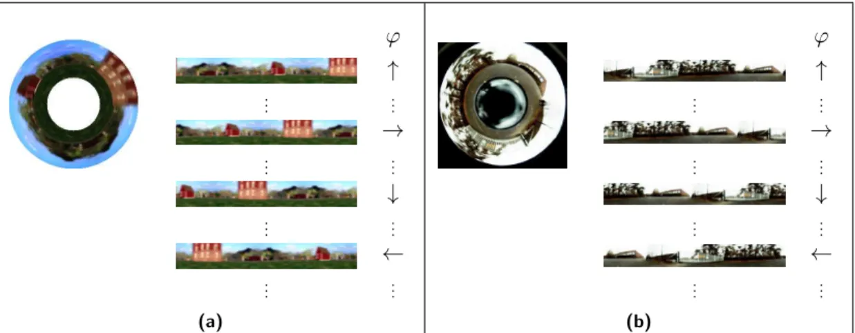
For the scenario of a robustly self-localizing and navigating mobile robot, we want to find functions that encode the robot’s position on the x- and y-axis as slowly varying features and are invariant with respect to its orientation. As stated in the previous section, learned slow features strongly depend on the movement statistics of the mobile robot during the training phase. In order to achieve orientation invariance, the orien-tation of the robot has to change on a faster timescale than its position. A constantly rotating robot with a fixed camera is inconvenient to drive, and a robot with a rotat-ing camera is undesirable for mechanical stability and simplicity. As an alternative, we use an omnidirectional imaging system which allows to easily add simulated rotational movement of the robot to manipulate movement statistics. Thus, the model is able to find orientation invariant representations of its own position without having to rotate the camera or the robot physically. During the training phase we simulate a full rota-tion for every captured image. Since for panoramic images a lateral shift is equivalent to a rotation around the yaw axis we can simulate a full rotation by shifting a sliding window over the periodic panoramic views (see Fig. 3.2 for an illustration). Throughout the experiments we use a window equal to 100% of the image size so that each rotated view contains the whole image, incrementally shifted along the lateral direction. Please note that achieving orientation invariance is a non-trivial task even when using a 100% window. An analysis of using windows of various sizes will be given in section 5.1.3.