Sequential Decision Making under Uncertainty for Sensor Management in Mobile Robotics

Sequential Decision Making under Uncertainty for

Sensor Management in Mobile Robotics

Julkaisu 1366 • Publication 1366

Tampereen teknillinen yliopisto. Julkaisu 1366 Tampere University of Technology. Publication 1366

Mikko Lauri

Sequential Decision Making under Uncertainty for

Sensor Management in Mobile Robotics

Thesis for the degree of Doctor of Science in Technology to be presented with due permission for public examination and criticism in Festia Building, Auditorium Pieni Sali 1, at Tampere University of Technology, on the 5th of February 2016, at 12 noon.

Tampereen teknillinen yliopisto - Tampere University of Technology Tampere 2016

ISBN 978-952-15-3676-2 (printed) ISBN 978-952-15-3701-1 (PDF) ISSN 1459-2045

Sensor management refers to the control of the degrees of freedom in a sensing system. The objective of sensor management is to improve performance e.g. by obtaining more accurate information or by achieving other operational goals. Sensor management is viewed as a sequential decision making process, where decisions at any time are made conditional on the past decisions and measurement data. At the time of deciding a control action for a sensing system the measurement data that will be obtained are unknown. Thus, informally speaking, a solution to a sensor management problem is a policy that determines which sensing action to undertake given the current information on the state of the process under investigation and contingent on any possible realisation of future measurement data outcomes.

This thesis studies sensor management framing the contingent planning problem in the partially observable Markov decision process (POMDP) framework. In particular, applications in mobile robotics are considered. Mobile robots are viewed as controllable sensor platforms.

Based on earlier work on POMDP based robot control, and distinguishing between the two cases of either exploiting or gathering information, we define four canonical sensor management problem types in mobile robotics. In each of the problem types, we exploit the structural properties of their inputs to improve efficiency of applicable contingent planning algorithms.

In particular, we consider sensor management problems for information gathering where the utility of the possible control policies is quantified by mutual information (MI). We identify the relationship between the POMDP formulation of an environment monitoring problem and another contingent planning problem known as a multi-armed bandit (MAB). In a robotic exploration task, we derive a novel approximation for MI.

Through both simulation and real-world experiments in mobile robotics domains, we determine the applicability, advantages, and disadvantages of a POMDP based approach to sensor management in mobile robotics.

During the course of this thesis project, I have had the privilege to interact with many inspiring people both at my home department of Automation Science and Engineering at Tampere University of Technology, and elsewhere. Without them the process would surely have been much harder.

I am sincerely grateful to my advisor, professor Risto Ritala. He has supported and guided me throughout the thesis process, and even earlier when I was not yet quite sure if I want to undertake such a project at all. He has been able to provide all the necessary resources for me to successfully pursue my research, and has succeeded in fostering a collegial atmosphere within the research group.

I have received a substantial amount of support from colleagues at the Department of Intelligent Hydraulics and Automation. For this, I want to acknowledge the head of the department, professor Kalevi Huhtala. Associate professor Reza Ghabcheloo has been tremendously helpful, offering his time for discussions and using his contacts to make my progress smoother. I have had many useful discussions also with others, of whom I especially wish to acknowledge Mika Hyvönen and Antti Kolu.

Associate professor Ville Kyrki from Aalto University and assistant profes-sor Matthijs Spaan from Delft University of Technology kindly agreed to pre-examine my thesis. Their careful reading of the thesis along with the comments and suggestions that helped improve the work are much appreci-ated. I also thank the anonymous reviewers of the journal and conference publications related to this thesis for their valuable feedback.

During discussions with my colleagues they have provided me with food for thought, challenging my initial ideas thus helping to improve them. Their concrete suggestions on experimental setup, along with their expertise on various technological issues has also been very helpful. For this, I especially wish to thank Marja Mettänen, Pekka Kumpulainen, Timo Salpavaara, Olli Suominen, and Joonas Melin. The many discussions on music and life in general with Marja and Pekka have helped make the workplace environment even more enjoyable and inspiring.

The financial support of the TUT President’s doctoral programme for funding my research between 2011 and 2015 is gratefully acknowledged. I thank the Finnish Society of Automation for providing travel grants that have allowed me to present my research results at various conferences and workshops. I am deeply thankful for the support my parents have provided to me throughout my studies. I also thank my brother Juho for his help in

proofreading the thesis. My girlfriend Saija has been there for me throughout the whole process. I could not have hoped for better support from all my friends and family.

Tampere, January 2016,

Abstract i

Preface iii

List of abbreviations ix

Notation xi

List of frequently used symbols xiii

1 Introduction 1

1.1 Uncertainty in decision making . . . 3

1.2 Decision theory and utility . . . 6

1.3 Sensor management . . . 8

1.4 Research questions . . . 10

1.5 Contribution . . . 11

1.6 Outline of the thesis . . . 11

2 Markovian systems and decision processes 13 2.1 Sequential decision processes . . . 14

2.1.1 Markov decision processes . . . 14

2.1.2 Partially observable Markov decision processes . . . . 16

2.1.3 Decision rules, policies, and optimality criteria . . . . 18

2.1.4 Optimal value functions and policies . . . 19

2.1.5 Classification of Markovian decision processes . . . . 21

2.2 Solving POMDPs . . . 22

2.2.1 Linear programming and policy iteration . . . 23

2.2.2 Point-based methods . . . 24

2.2.3 Problem compression . . . 27

2.2.4 Online methods . . . 28

2.2.5 Other approaches . . . 41

2.2.6 General POMDPs . . . 44

2.2.7 Summary of POMDP solution methods . . . 46

2.3 Markovian multi-armed bandits . . . 48

2.3.1 Partially observable MABs . . . 49

2.3.2 Index policies for MABs . . . 50

3 Canonical sensor management problems in mobile robotics 53 3.1 Motivation for information-theoretic reward functions . . . . 53

3.2 POMDPs applied to problems in robotics domains . . . 55

3.3 Overview of the canonical sensor management problems . . . 57 v

3.4 Deterministic robot motion and mixed observability . . . 59

3.4.1 Robot motion model . . . 59

3.4.2 Markovian model for environmental variables . . . . 60

3.4.3 Path planning . . . 63

3.4.4 Environment monitoring . . . 65

3.5 Stochastic robot motion and partial observability . . . 65

3.5.1 Task support . . . 66

3.5.2 Robotic exploration . . . 67

4 Solving sensor management problems 71 4.1 Selection of POMDP solvers for sensor management problems 72 4.1.1 Path planning . . . 72

4.1.2 Environment monitoring . . . 73

4.1.3 Task support . . . 74

4.1.4 Robotic exploration . . . 75

4.2 Heuristics and bounds for path planning . . . 75

4.2.1 Upper bound for leaf nodes . . . 76

4.2.2 Heuristic value for leaf nodes . . . 76

4.3 Multi-armed bandit relaxations for environment monitoring . 77 4.3.1 Relaxed environment monitoring problems . . . 78

4.3.2 MAB equivalence of problem relaxations . . . 79

4.3.3 Computing the upper bound . . . 88

4.4 Value iteration in continuous-state task support . . . 91

4.4.1 Error bound for point-based value iteration . . . 92

4.4.2 Constructing a set of belief points for point-based value iteration . . . 94

4.5 Mutual information in robotic exploration . . . 94

5 Case studies 99 5.1 Path planning . . . 99

5.1.1 Independent environment variables . . . 100

5.1.2 Avoiding moving obstacles . . . 102

5.2 Environment monitoring . . . 105

5.2.1 Problem definition . . . 105

5.2.2 MAB conditions satisfied . . . 106

5.2.3 MAB conditions violated . . . 110

5.3 Task support . . . 112

5.3.1 Problem definition . . . 112

5.3.2 Comparison of GMM component reduction methods . 114 5.3.3 Policies and the value of information . . . 117

5.3.4 Comparison with sampling-based planning . . . 119

5.4 Robotic exploration . . . 120

5.4.1 Operating a camera system . . . 120

5.4.2 Exploration of unknown environments . . . 128

5.4.3 Simulation . . . 129

5.4.4 Implementation . . . 135

5.4.5 Experimental validation . . . 136

6 Discussion and conclusion 143 6.1 Summary of results . . . 143

6.3 Discussion and future work . . . 146

Appendix A Information theory 147

A.1 Entropy and conditional entropy . . . 147 A.2 Relative entropy and mutual information . . . 148

Appendix B Gaussian mixture model simplification 151

B.1 KL divergence . . . 151 B.2 Infinity norm . . . 152 B.3 L2 _{norm . . . 152}

Appendix C A lazy sampling scheme for robotic exploration 155

Bibliography 157

CTP Canadian traveller’s problem. DAG directed acyclic graph.

DBN dynamic Bayesian network.

E-PCA exponential family principal component anal-ysis.

EKF extended Kalman filter. FIB fast informed bound. GMM Gaussian mixture model. GPS global positioning system. HMM hidden Markov model.

HSVI heuristic search value iteration. KL Kullback-Leibler.

LQG linear-quadratic-Gaussian. LRF laser range finder.

MAB multi-armed bandit. MC Monte Carlo.

MCTS Monte Carlo tree search. MDP Markov decision process. MI mutual information. MPC model predictive control. OLFC open loop feedback control. PBVI point-based value iteration. PDF probability density function. PMF probability mass function.

POMCP partially observable Monte Carlo planning. POMDP partially observable Markov decision process. PWLC piecewise-linear and convex.

RBPF Rao-Blackwellized particle filter. RHC receding horizon control.

ROS Robot Operating System. RTBSS real-time belief space search.

SLAM simultaneous localization and mapping. SMC sequential Monte Carlo.

UCT upper confidence bounds for trees. UMDP unobservable Markov decision process.

Dpp, qq Kullback-Leibler (KL) divergence between two PDFs ppxqand qpxq.

EX mathematical expectation under X „ ppxq, also _E if probability density function (PDF) or probability mass function (PMF) is clear from context.

G“ pX, Eq an (un)directed graph with vertices X and (un)directed edgesE.

HpXq entropy of a random variable X.

HpX |Yq conditional entropy of a random variable X

given a random variable Y.

IpX;Yq mutual information of random variables X

and Y.

1X A stochastic identity mapping on the set X. Specifically, for x1, x2 P X :1Xpx1, x2q “1 if

x1 “x2 and 0 otherwise.

Mpx, dq given a graph G“ pV, Eq, the subset of ver-tices reachable fromxP V by a path of length

at mostd.

Npxq given a graph G“ pX, Eq, the set of vertices

neighbouringxPX.

Npx;m, Pq a Gaussian PDF over random variableX with mean m and covariance matrix P.

ppxq a PDF or PMF of a random variableX at x.

ppx|yq a conditional PDF or PMF of a random

vari-able X atx, conditioned on another random variable Y “y.

PpXq the set of all PDFs or PMFs over the set X.

2X the power set of set X.

xt a variablex indexed by an index t.

xi:j a variable x indexed by an index range from

i toj, if iąj, interpreted as empty.

X a random variable.

x a realisation of a random variable X, or a member of a set.

X the domain of a random variable X, or a set.

X „ppxq a random variable X distributed according to a PDF or PMF ppxq.

a a decision or action. A action space.

b a belief state, a PDF or PMF over the state. B set of beliefs, the set of all PDFs or PMFs over

the state space.

d typically a positive integer denoting search depth in a tree search.

γ discount factor.

G generative model of a POMDP,G :SˆBˆ

AÑS ˆZ ˆR.

h a history sequence of actions and observations. H set of all possible history sequences.

m a realization of a map in a robotic exploration problem.

M the set of possible realizations of a map in a robotic exploration problem.

O a probabilistic observation model, O : Z ˆ

SˆA Ñ r0,1s.

δ a decision rule, δ:BÑA.

π a policy; a sequence of decision rules.

π˚ _{an optimal policy.}

Π space of admissible policies.

ρ a reward function, ρ:BˆAÑR. R a reward function, R:SˆAÑR. s state of a system.

S state space.

t an decision epoch or index. T set of decision epochs or indices.

τ belief update equation,τ :BˆAˆZ ÑB.

T a stochastic state transition model, T : S ˆ

AˆS Ñ r0,1s.

Vπ the value function of a policy π,Vπ :BÑR. Vπ˚ _{the value function of an optimal policy, V}π˚ _:

BÑR.

Q aQ-value function, Q:BˆAÑR.

Jd an open loop value function for a look-ahead depth of ddecison epochs, Jd:BˆAdÑR.

x fully observable part of states“ px, yq, or the

robot pose in a robotic exploration problem. X the fully observable part of a mixed observable state space S “X ˆY, or the pose space in

an robotic exploration problem.

y partially observable part of state s“ px, yq.

Y the partially observable part of a mixed ob-servable state space S “X ˆY.

z a data sample or observation. Z observation space.

Introduction

Sensing systems have become a part of everyday life, and humans today live in an environment with an unprecedented number of sensors. Among other variables, the sensors may monitor the properties of the environment, e.g. the temperature, or the humans themselves, e.g. their heart rate. The sensors are often able to communicate the results of their sensing activities over a network connection for remote access. Likewise, the decreasing price of sensors and increased ability to communicate sensing results has reinvigorated sensing in industrial processes, helping provide information on parts of the process that could not be investigated earlier. Yet another application for deploying sensing systems has emerged with the appearance of mobile robots. Mobile robots are equipped with sensors which enable them to obtain information about areas that are currently not reachable by humans or human-operated vehicles. Examples of such activities include deep sea exploration and study of other planets of our solar system. Modern sensors are often agile, meaning that they have multiple possible operating modes, selected by software commands – consider for instance cameras that can be panned and tilted, or a radar whose beam may be steered by controlling the phase of the electrical input signals to its antenna array. As availability of sensor data has increased, questions on how to manage the collection of the data have become increasingly important. Which temperature sensors should be activated to collect most useful data if we wish to estimate the temperature in a given area? Which operating modes should be chosen for a camera to detect an object of interest? Where should a deep sea mobile sensor platform move to most accurately model the underwater currents and environment? To give justified answers to these types of questions, analysis of the possible decisions and their effects in the context of the sensing system is required. Results of the analysis have the potential to reduce energy consumption, e.g. by reducing the distance a mobile sensor platform needs to travel, and to improve efficiency of executing tasks by reducing the required time, while simultaneously maintaining or even improving the quality of information obtained.

Systems, both human-designed and others, can be characterised using the concepts of state, action, and observation. The state may be thought of as a minimal representation of all internal features relevant to the function of the

system that are required to distinguish different conditions of the system from one another. An action is an external stimulus affecting the system, and an observation is a perceived response from the system conditional on the state. An observation may arise spontaneously without an action affecting the system, but it may also be affected by the action. As a simple example, consider a systems view of making a telephone call to a friend. The caller provides an action by dialling a number on their telephone. Conditional on the state of the line dialled, the caller observes feedback either in the form of a dialling tone or a signal denoting the line as busy. If the line is not busy, the caller may wait for the call to be accepted, which is observed by hearing the receiver of the call answer.

The definition of a system may vary: instead of the states of the two telephones, one could consider the state of the system as the state of the friend, for instance whether they are busy, at home, or at work. One could also consider text messages besides telephone calls as actions. The definition of an observation could then also include the fact whether the friend replied to the text message.

The state of a system is often partially observable; one may only infer it incompletely based on the perceived observations. For example, suppose you call a friend but your call is not answered. You could for instance deduce that they are busy and unable to talk, or that they have not even observed that you tried to call them and hence did not answer.

A decision making task can be defined as providing stimuli to a system in such a manner that the observed feedback implies a desirable state of the system from the point of view of the values and preferences held by the decision maker. For example, suppose again you wish to talk to your friend. From this perspective, it is desirable to dial the friend’s telephone and wait for them to answer the call. Note also that a decision making process does not always prompt action: once you have finished talking to your friend you decide, content with the chat you just had, to not take any further action. Decision making is a central element of almost all human activity, ranging from financial investment and military decisions to social behaviour in a group. The end result of the decision making process outlined above, a transition from an initial state to a desirable final state after the decisions have been acted upon, is also a key feature of automatic control. Consider controlling the flow rate of a liquid in a pipe by means of a valve that may be adjusted by an electrical motor. A simple proportional feedback controller can automatically control the flow when a measurement of the current flow rate is compared to the preferred flow rate, called a set point. The controller then produces a decision – a control signal to the electrical motor – proportional to the difference between the measured value and the set point.

This thesis studies decision making under uncertainty in the context of control of automated systems. The formal methods applied for representing decision making problems are contained within the rubric of decision theory. Of particular interest are decision making strategies applicable for sensor management, i.e. decision making for controlling sensors with user-selectable operation mode or scheduling operation of a network of possibly hetero-geneous sensors. The primary application area considered in the thesis

are mobile robots. Out of the general requirements a robot control sys-tem should satisfy (Alami et al., 1998), we focus on enhancing autonomy

by studying methods that enable robots to independently carry out their assigned information gathering tasks.

Technical context. In the following sections, the three key elements of the thesis; uncertainty in decision making, decision theory, and sensor manage-ment are discussed in more detail. The subjects are discussed in the specific technical context ofdiscrete-time Markovian stochastic systems(Albin, 2003). This entails the following assumptions:

A1: The state of the system under investigation evolves and decisions are executed sequentially, such that the state at the next time instant depends only on the current state and decision, and A2: mathematical, stochastic system models are available for the

state transition and observation processes.

Decision-making throughout the thesis is considered from a single-agent

perspective, formalizing the problem mathematically as a partially observable Markov decision process (POMDP). However, further discussion on POMDPs is deferred to Chapter 2.

After detailed discussion of the key elements, this chapter is concluded by presenting the research questions studied, describing the contribution of the thesis with respect to the research questions, and providing an outline of the rest of the thesis.

1.1

Uncertainty in decision making

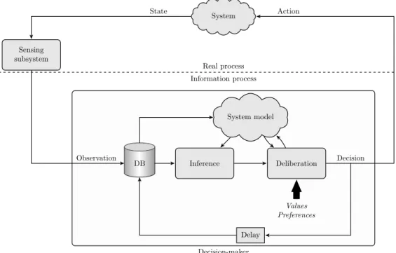
Figure 1.1 illustrates decision making as a continuous process. The decision maker is located within the box on the lower part of the figure, and the system that is being acted upon is located at the top of the figure. The decision maker and the system can be viewed as two agents communicating via actions and observations.

The main parts of the system are separated by a dashed horizontal line. The real process, located above the dashed line, depicts the real system being acted upon, e.g. the telephone in the example of the previous section. In the information process, located below the dashed line, the primary activity is processing of information contained in the perceived observations from the system, and making decisions based on the information. In the case of a human decision maker, this part depicts the thinking process that precedes acting upon decisions. On the right hand side of the figure, the dashed line represents an interface between decisions andacting on them. On the left hand side, the dashed line represents an interface between the actual state of the system and the perceived observations.

The type of the interfaces depends on the decision making task and also on how the boundaries of the system itself were defined. In the telephone example one could for instance place the decision-action interface either between the telephone dial and the caller’s finger, or at the transfer of neural

impulses from the decision maker’s brain to the muscles ultimately dialling a number. The former interface is at the physical separation between the system and the decision maker’s embodiment, while the latter corresponds to setting the interface at the point where thinking activity first prompts an observable action that affects the system. Similarly, the sensing subsystem acting as a state-observation interface could be contained within or outside of the decision maker’s embodiment. In the telephone example, the sensing subsystem is the auditory perception sense of the caller, contained within their embodiment. For the discussion in this section, we consider the sensing subsystem as external to the decision maker, passively interfacing states to observations without the decision maker being able to affect the process (other than indirectly through perceiving the effects of actions on the actual system). We return to the question of controllable sensing subsystems later in Section 1.3. Decision-maker DB Inference System model Deliberation Values Preferences Delay Decision Observation Sensing subsystem System Action State Real process Information process

Figure 1.1: Decision making as a continuous process.

Assuming the system being acted upon is fixed, for the remainder of this section we will concentrate on the process of decision making, i.e. the information process in the lower part of Figure 1.1. A decision is made following a three-step process. First, the perceived observation from the system and the previous decision are stored into a database (DB), located on the left hand side of the decision maker box. The database is a representation of the past experiences of the decision maker, a history of decisions and observations. Second, the information currently stored in the database is applied to infer the state of the system being acted upon. Finally, a deliberation that results in a decision is executed, based on results of inference and the decision maker’s values and preferences.

The information in the database is interpreted in the context of the system model, as illustrated by the arrow pointing from the system model towards inference. The system model represents, in the case of a human decision maker, his or her understanding of the inner workings of the system. In the case of automatic systems, the model is typically a mathematical object

representing the relationship between states, actions, and observations. The system model is needed since the actual system may be hidden from the decision maker, the only interaction allowed being via the actions and observations. As such, the model is subject to uncertainty: it may well be that the decision maker has an incomplete understanding of the functioning of the system. Thus, it is also desirable in some cases to adapt the system model based on the decision maker’s past experiences. This is illustrated by the arrow pointing from the database towards the system model.

Even if the system model were exact, inference is subject to uncertainty if the observations do not allow unambiguous inference of the system state, or conversely, if perception is not perfect. The former case may arise if more than one state can produce the same observation, and the latter case is encountered for instance when observations are being measured by a noisy sensor. Consider the flow rate example presented earlier, where the state of the system is the rate of flow in the tube. A measurement of the flow rate provides an answer to the question, “What is the flow rate in the tube?” However, as measurements are affected by random noise, unknown biases, and other such phenomena, the information about the state provided by a measurement is always incomplete.

According to normative models of decision making, a decision maker acts rationally when their preferences are not circular, i.e. if they prefer outcome

a to outcomeb and in turnb to c, it should follow that they also prefer a

to c(French and Ríos Insua, 2000). Descriptive models of decision making represent actual human decision making processes, and it has been shown that humans are afflicted by a variety of biases and heuristics leading to irrational behaviour and errors in judgement (Tversky and Kahneman, 1974). Under assumption of non-circular preferences, Figure 1.1 is a suitable normative description of decision making in automatic systems. The figure also incorporates the view that the decision maker’s values or preferences do not affect their inference.

In the deliberation stage, the decision maker reflects the values and prefer-ences they hold against the effects of decisions as predicted by the system model, given the information about the current state of the system ob-tained as an output of inference. The process is often iterative, consisting of evaluating various possible future courses of action. This is illustrated in Figure 1.1 by the two-way arrows between the deliberation block and the system model. The effects of decisions cannot always be predicted with complete precision. This is the case especially in stochastic systems, that may respond to the same action in different ways depending on random chance. Stochasticity may arise for example when there are phenomena whose effect on the state of a system is unknown but significant, or when the system model is simplified such that the state does not account for all aspects of how the system functions and thus cannot fully predict its response to an action.

We conclude that uncertainty in decision making manifests itself as incom-plete knowledge of the current state, incomincom-plete answers to attempts to gain information about the state, or lack of certainty about the effect of a decision. As discussed, uncertainty may arise because of modelling errors or other reasons. Generally, a decision making task can feature uncertainty

from any subset of the three manifestations.

Depending on the decision making task, some or all of these sources of uncertainty can sometimes be ignored. If uncertainty cannot be ignored, principled methods of coping with it are required.

1.2

Decision theory and utility

“. . . the class of statistical problems in which the statistician must gain information about certain critical parameters in order to be able to make effective decisions in situations where the consequences of his decisions will depend on the values of these parameters.” (DeGroot, 2004)

Considering the discussion of decision making above, the parameter on which the consequences of decisions depend is the state of a system. Information about the parameters refers to inference on the contents of the database, and helps the decision maker to act in a manner that best agrees with their values and preferences.

Assuming that the information about the system state is incomplete, a probability value depicting the relative likelihoods that the system resides in a state may be assigned to each possible state. This assignment effectively provides a mathematical quantification, in the form of a probability density function (PDF) over the space of possible states of the system, of the

uncertainty the decision maker is currently experiencing about the state; the value of the above mentioned critical parameter upon which the consequences of their decisions depend. A complementary but fundamentally equivalent way to understand the PDF is as representation of the information currently available to the decision maker about the state of the system. The PDF is often called a belief state. Other methods for representing uncertainty include e.g. fuzzy sets, but they are not considered further in this thesis. When decisions are implemented as actions and consequential observations are perceived, a mathematical engine for revising existing information is required. When information is represented as a PDF and a mathematical system models for the state and observation process are available, Bayesian filtering (Särkkä, 2013) is applied for revising it. Bayesian filtering consists of a prediction and an update step. In the prediction step, a mathematical model of the system state conditional on the previous state and action is applied to propagate current information into a prediction of the resulting state. This model is often called the dynamical model of the system. Once an observation is perceived, another mathematical model of the observation conditional on the current state and previous action is applied to incorporate information provided by the observation into the state information. This model of the perception process is often called the observation model of the decision maker. From the point of view of the decision maker, these two models, along with any possible prior information, are sufficient to infer a PDF on the current system state based on the history of past actions and observations.

When the values and preferences of the decision maker are likewise quantified, e.g. as a function that assigns a numerical value for each pair of state and action, the desirability of various courses of action may be compared in an objective1 _{manner. This forms the basis of statistical decision theory; see} e.g. Raiffa and Schlaifer (2000); DeGroot (2004).

The application of statistical decision theory typically results in finding a policy, a prescription of which course of action is to be taken given e.g. the current belief state. An optimal policy is the one which, when followed, will produce an outcome that is the best achievable given the notion of optimality applied in the analysis. One commonly applied definition of optimality is given by the theory of expected utility of Von Neumann and Morgenstern (1953), who showed that if there exists a complete ordering of the preferences of possible outcomes, then there exists a utility function that quantifies the desirability of states and actions, and that the decision maker prefers actions that maximise the expected value of the utility function. The expected value of the utility function is calculated under the aforementioned probability density function quantifying the likelihood of each state. Other possible notions of optimality include e.g. maximising the probability of the system reaching some desirable state, or minimising the probability of an adverse state. For the remainder of the thesis, we adopt maximising expected utility as the notion of optimality.

Often, decisions have both short-term and long-term consequences. When a single decision is considered, an optimal decision may be found by maximising the expected value of the utility. However, focusing on optimality over a single decision may not be sufficient. For instance, a cross-country skier in a long race considering performance only along the next hundred meters will likely not fare well. Instead, both the present and future decisions and their possible outcomes should be considered at the time of decision making. The time frame over which future outcomes and decisions are considered thus also affects the outcome of finding an optimal decision.

The problem of maximising expected utility over multiple decisions has been central in the field of dynamic programming (Bellman, 1957). Bellman’s principle of optimality, which states that for an optimal course of action, “whatever the initial state and initial decision are, the remaining decisions must constitute an optimal policy with regard to the state resulting from the first decision”, is leveraged to break the multi-stage decision problem into simpler sub-problems. A backward recursive procedure is applied by which the maximal expected utility along with the decision that leads to it may be recovered for any number of remaining decisions after the current one. Not every optimal decision problem has the property that allows this to be done – a utility value must be assignable to each individual decision for dynamic programming to be applicable. In our context of Markovian systems, this requirement translates to a utility value being assigned to each pair of state and decision, with the additional requirement that the decision-maker instantaneously receives this reward as a result of the decision.

The complexity of the problem increases as the number of possible states in the system increases, an issue termed the curse of dimensionality. Reasoning 1_{Provided the decision maker’s values and preferences themselves are not reflective of} any biases.

over long time horizons constitutes a major source of computational difficulty in both dynamic programming and mathematical decision theory in general. Statistically optimal decisions are analysed with the aforementioned math-ematical models of the system, i.e. the models are applied within the de-liberation loop in Figure 1.1. Thus when we discuss optimal decisions, we refer to optimality with respect to the mathematical model of the system applied unless otherwise specified. As explained e.g. by Kaelbling et al. (1998), it may seem counter-intuitive that the decision maker achieves a

large expected utility merely bybelieving it is in a good state, i.e. attaining a belief state where it is in a preferred state with high probability. However, if the system models are correct, there is no discrepancy between the expected rewards under the decision maker’s belief state and the true expected rewards considering the real system. When models cannot be assumed correct, spe-cial care must be exercised when results obtained from a decision-theoretic optimisation are applied; especially when there is a risk of great negative effects from bad decisions.

1.3

Sensor management

Sensor management refers to “. . . control of the degrees of freedom in an agile sensor system to satisfy operational constraints and achieve operational objectives” (Hero and Cochran, 2011). As such, sensor management in automatic systems is intimately related to decision making. The system under study is a sensor itself, or a sensor subsystem of a larger system having also other functions. The operational objectives refer to the values and preferences of the decision maker, expressed e.g. as a utility function. Resource constraints often prevent simultaneous use and processing of all available measurement data. Although more data processing resources are available today than ever before, the demand for sensor management has simultaneously increased due to technological developments in both sensor technology and communication networks.

As software has become an increasingly important part of modern sensor technology, the agility of sensors has increased dramatically. Multiple degrees of freedom are available for operation of sensors. By allowing rapid changes to the configuration of the sensor via software commands, the traditionally monolithic sensor has been transformed into an array of virtual sensors, each corresponding to a single configuration. Examples include cameras whose focus can be switched to a certain part of the visible scene and radars with variable signal waveform or transmission frequencies.

Another advance in sensor technology over the last decades has been the increasing availability and decreasing cost of increasingly more capable sensors. For instance, a modern mobile phone for consumer use typically has sensors for imaging, detecting tactile inputs, and measuring the position and inertial state of the device.

When sensors are carried by a mobile platform, even more degrees of freedom are introduced to the operation of the sensor subsystem. Mobile sensor platforms that are remotely operated or working autonomously have allowed measurement campaigns in environments where human presence is either

impossible or undesired. Examples include deep ocean measurements, ex-ploration of other planets of the solar system, and other long-lasting data collection missions in remote or hazardous locations.

Advances in communication networks and infrastructure mean that also the availability of remote access to the data produced by the sensors has improved considerably. With the present emphasis on increasing connectivity of individual devices through concepts such as the Internet of Things, the trend of increasing availability of sensor data is likely to continue.

The increasing number of agile sensors may produce data in quantities that are not possible to analyse fully, given constraints on available computing power or time required by the analyses. When multiple sensors are available, it may sometimes be impossible to operate all of them concurrently, or operation may be restricted to certain subsets of sensors at a time. Possible reasons for such restrictions include conflicts in use of the electromagnetic spectrum (e.g. in case of radars), or limited bandwidth to communicate the data to the user. Likewise, it is desirable to operate the sensor in such a way that the operational objectives are most effectively reached; minimising e.g. the time or resources spent. All these factors have contributed to an increasing need for sensor management in automatic systems.

As this thesis considers decision making for controlling sensors, the aspect mentioned in the quotation in the beginning of Section 1.2 about experiments providing new information about the state is particularly interesting. In the context of automated systems, new information typically arrives in the form of measurement data from sensors. From the point of view of sensor management, the objective can be either operating a sensor system to gather the greatest possible amount of information about the system state, or to support execution of a task that is not necessarily related to sensing per se. This has important implications for the utility function of the decision making problem. If the preference of the decision maker is e.g. to reach a certain state in the system, it is sufficient to formulate the utility function as dependent on the state only. Then, an optimal course of action is to gather information only up to the extent that the information best helps to achieve the aforementioned preferred state. However, when information gathering itself is an objective, it is in general not possible to formulate the utility function as purely state-dependent: which state the system resides in is often independent of the decision maker’s knowledge. Instead, the utility function is defined directly in terms of the belief state: a small utility is assigned to uncertain belief states, and a high reward to certain belief states where probability mass is concentrated on few underlying states.

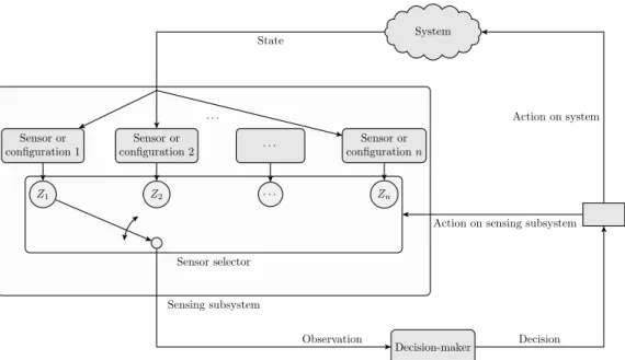
Figure 1.2 provides a schematic view of the decision making process in a sensor management problem. The figure may be seen as equivalent to the general view of Figure 1.1, however, we have chosen to show this alternative representation to facilitate discussion on aspects specific to sensor manage-ment problems. We again view the sensing subsystem as external to the decision maker, although the resulting analysis is fundamentally the same even for an embodied sensing subsystem.

The sensing subsystem shown on the left hand side of Figure 1.2 consists ofn

sensors labelled by consecutive integers from 1 to n. Depending on the case these sensors may either refer to multiple distinct sensors, or represent the

Sensing subsystem Sensor selector Z2 . . . Z1 Zn Sensor or configuration 1 Sensor or configuration 2 . . . Sensor or configurationn . . . Decision-maker Observation System State Decision Action on sensing subsystem

Action on system

Figure 1.2: Sensor-management as a decision making problem.

multiple configurations that a single sensor may be operated in. Each sensor 1ďiďn provides an observation Zi conditional on the state of the actual system. A sensor selector, presented on the bottom of the sensing subsystem, selects which sensor’s observation will be recorded by the decision maker. The sensor selector may either select a single sensor or a subset of them at a time, by connecting them with the system on the top of the figure. The possible configurations the sensor selector can choose are such that the physical and other constraints outlined in the paragraphs above are satisfied. The sensor selector can be acted upon by the decision maker to choose which sensor’s observation to perceive next. In the general case, the decision maker is jointly applying control actions on the system itself, and actions on the sensing subsystem to control the observation process. In case the decision maker has no control over the evolution of the system state and is merely an observer, the arrow connecting the decision maker to the system is removed. If the system state cannot be acted upon, the utility function must depend on the decision maker’s belief state: if it did not, no action on the sensing subsystem could affect the state of the actual system and hence the reward, rendering the resulting optimal decision problem meaningless.

1.4

Research questions

This thesis investigates the application of model-based methods for decision making under uncertainty, applied to sensor management. In particular, the subset of Markovian systems with hidden state, also called partially observable Markov decision processes (POMDPs) is studied. The two cases where utility is measured by either a state or belief state dependent function are considered. Mobile robots are considered as the primary application area.

RQ 1: How should sensor management problems be formulated as POMDPs?

RQ 2: Which structural properties of sensor management problems can be taken advantage of to tailor existing exact and approximate algorithms for solving POMDPs to be efficient in solving sensor management problems in mobile robotics?

RQ 3: For the approximate methods considered, what guarantees on the quality of the solution can be provided compared to the optimal solution?

1.5

Contribution

The objective of the thesis is to discuss alternative formulation of sensor management problems in mobile robotics as POMDPs, to identify structural properties of sensor management problems that can be exploited in finding a useful solution more effectively, and to demonstrate the applicability of POMDP-based sensor management in the domain of mobile robotics. In view of these objectives, the contributions of the thesis are as follows.

• A comparison of state-of-the-art algorithms for solving POMDPs applied to sensor management problems is provided.

• Based on a review of existing work on applying POMDPs to control of real robots, a set of canonical sensor management problems relevant in mobile robotics is defined, and suitable algorithms for solving the problems are identified. The applicability is empirically verified via simulation.

• For each of the canonical problems, structural properties that can be exploited in solving the problem are identified. In particular,

– For problems with a state dependent utility function, bounds and heuristic approximations for the optimal value function are provided.

– For problems with a utility function that is non-linear in the belief state, connections to multi-armed bandit problems are identified.

• Applicability of a POMDP-based approach to sensor management in autonomous robotic exploration of an unknown environment is demonstrated.

1.6

Outline of the thesis

The thesis is organised as follows. Chapter 2 reviews the state-of-the-art of partially observable Markov decision processes and multi-armed bandits. Chapter 3 formulates four canonical sensor management problems in mobile robotics domains for this study. Necessary background information on graphs and graphical models is also provided. Chapter 4 gives the main contribution

of the thesis. Features of the canonical problems and suitable POMDP solution techniques are analysed. Exploiting structural features of each canonical problem type is described. Chapter 5 validates the analysis of the previous chapters and provides empirical comparison between suitable solvers for the canonical problems via simulation experiments. A sensor management system applied to autonomous robotic exploration is described, and the system is validated in a real world exploration task. Finally, Chapter 6 provides discussion of the results and concludes the thesis.

Markovian systems and decision

processes

As discussed in the Chapter 1, sensor management may be seen as a decision-making process. Markov decision processes (MDPs) are a subset of general stochastic decision processes, with the distinction that the effects of decisions depend only on the decision-maker’s action and the current state of the system. This property, known as the Markov property, may be interpreted as a lack of memory in a stochastic process.

The Markov property is a useful assumption in modelling sequential data. Sequential data models are applied in a wide range of applications, ranging from text or speech recognition (Bishop, 2006), modelling of biological signals such as sequences of nucleic acids (see e.g. Eddy, 1996) to tracking targets by radar (Moran et al., 2008).

The Markov property is often justified from a practical point of view and many stochastic processes that do not satisfy the Markov property can be well approximated assuming they do (Albin, 2003). Systems with a finite memory longer than a single time step may be transformed into Markovian systems with one-step memory by state augmentation. In decision processes, the Markov property together with a suitable objective function allows solutions based on dynamic programming methods (Bellman, 1957). The objective of this chapter is twofold. The first objective is to provide background information on the mathematical formulation of decision-making processes that can model sensor management problems. This facilitates further discussion on problem formulation in subsequent chapters. The second objective is to identify which optimal or approximate algorithms for finding solutions to Markovian decision processes are most relevant for sensor management problems.

Markov decision processes are defined in Section 2.1. Both fully observable states and partially observable states are considered. The latter is especially important for sensor management applications. Section 2.2 reviews the state-of-the-art in solving Markov decision processes with partially observable state. The chapter is concluded in Section 2.3 by giving the definition of a related decision process model called a multi-armed bandit (MAB).

2.1

Sequential decision processes

In a stochastic decision process, an agent sequentially applies actions on the process and perceives their effects. The process is called stochastic, as the action effects are not known exactly, but rather a PDF over the possible effects is available. In this section, we consider discrete-time Markovian decision processes. The motivation for this choice is principally practical; tractable solutions are available for discrete-time decision processes corresponding to realistic problems. For an overview of continuous-time stochastic decision processes we refer the reader to the classic book of Åström (1970) on stochastic control theory.

We give definitions for discrete-time Markov decision processes with both fully observable and partially observable state. Partial observability means that the state of the process is not directly observable, but rather information about the state is obtained via noisy or incomplete observations. Partial observability is an especially useful feature for modelling sensor management problems.

Subsections 2.1.1 and 2.1.2 define the sequential decision making framework with full and partial observability, respectively. Discussion on how to act optimally in the context of this framework is deferred to Subsection 2.1.3, including formalisation of decision rules and policies. The basic recipe for finding optimal policies via dynamic programming is presented in Subsec-tion 2.1.4. Finally, SubsecSubsec-tion 2.1.5 presents a brief taxonomy of Markovian decision processes and their relation to each other, including cases with multiple decision-makers.

Notation. Throughout the text, we denote random variables by uppercase italic letters, e.g.X. The space of possible realisations of a random variable

X is denoted by a calligraphic letter, e.g. X. A similar calligraphic notation is adopted for sets. Members of sets and realisations of random variables are denoted by lowercase italic letters, e.g. xPX. Sequences are denoted as pxkqiďkďj ”xi:j. If a continuous random variable X is distributed according to a given PDFp:X ÑR`, we writeX „ppxq. For brevity, we occasionally denote different PDFs by the same functionp – in this case, the arguments of the function distinct which PDF is referred to by each expression. The space of all possible PDFs over X is denoted byPpXq. For discrete random variables and their probability mass functions (PMFs) over finite sets, we adopt a similar notation.

2.1.1

Markov decision processes

Throughout this section, we assume that the realisations of all random variables can be completely observed. We define a stochastic process which satisfies the Markov condition. After defining a controllable Markov process, we ultimately define a Markov decision process.

Definition 2.1 (Stochastic process). A stochastic process is a collection of random variables tStu indexed by time tPT, where T is an index set.

The index setT typically models time and can be either discrete or continu-ous, e.g. T “ t0,1, . . .u or T “ tt P R| 0ď t ă 8u, respectively, or some closed interval subset of either.

Consider a discrete-time stochastic process tStuwith T “ t0,1, . . .u. Each

St models the system state at time t and assumes values in a state space S. In a general causal stochastic process, St`1 may depend on the realisations of anySk,k ďt. This leads to a state transition model defined as a conditional PDF ppst`1 | st, st´1, . . . , s0q. Note that we assume the state transition model to be independent of t. This assumption is made to simplify notation, and no conceptual difficulties arise from defining state transition models dependent on t, as is done e.g. by Puterman (1994).

When dependency on past states is reduced toSt only, a Markov process is defined.

Definition 2.2 (Markov process). A discrete-time stochastic process tStu

with T “ t0,1, . . .u is a Markov process if its state transition model satisfies

the Markov condition

ppst`1 |st, st´1, . . . , s0q “ppst`1 |stq (2.1)

for all tP T and all s0, s1, . . . , st`1 PS.

In a decision process, an agent has the opportunity of influencing a stochastic process by applying actions. Fundamentally this means that the state transition model of the process is an action-dependent function. Actions can be selected at the decision epochs determined by an index set T. If T “ t0,1, . . .u, the decision process is of infinite horizon. IfT “ t0,1, . . . , du,

d PN, the decision process is of finite horizon, and the last decision is made

at epoch pd´1q. If at some decision epoch the system is in state sP S, the agent may choose the action to apply from the set of actions allowed in s, denoted As. LetA “

Ť

sPS

As denote the action space of the decision process. With the introduction of actions, a controlled stochastic process is defined, where in general the next state depends on the past state and actions both via a state transition model ppst`1 | st, st´1, . . . , s0, at, at´1, . . . , a0q. In a controlled Markov process, state transitions satisfy the Markov condition with respect to the states and actions.

Definition 2.3(Controlled Markov process). In a controlled Markov process, the state transition model satisfies

ppst`1 |st, st´1, . . . , s0, at, at´1, . . . , a0q “ ppst`1 |st, atq (2.2)

for all tP T and all s0, s1, . . . , st`1 PS, a0, a1, . . . , atPA.

The state transition model in a controlled Markov process is concisely represented as a function _T:SˆAˆS ÑR`, such that Tps1_{, a, sqis the}

value of the PDF over the new system state s1 _{when the system is currently}

in state s and action a is executed. A valid state transition model must satisfy ş

S

Tps1_{, a, sqds}1 _{“1 for all sPS and aPA}1_. 1_{For finiteS,}

The actions are applied in a sequential manner. At decision epoch t, the system is in a statest. The agent then executes action at, and the system transitions to a new statest`1 according to T. The agent receives a reward

R1

pst, at, st`1q, which is a random quantity as it depends on the system state at decision epoch pt `1q. The reward function is assumed to be independent of the decision epoch, although no extra difficulty beyond notational inconvenience arises from epoch-dependent rewards. Positive reward is interpreted as an income, and negative reward as a cost. We adopt the alternative view of the reward function R1 _{where it is replaced by its}

expected value calculated by

Rpst, atq “ESt`1rRpst, at, st`1qs, (2.3) defining a new expected reward functionR :SˆA ÑR. The expectation

in the expression above is taken with respect to _T ” ppst`1 | st, atq. In a finite-horizon decision process with T “ t0,1, . . . , du, the last action is selected at decision epoch pd´1q, and an additional real-valued terminal

reward Rdpsdqis sometimes defined. Throughout the rest of the thesis we assume the terminal reward is equal to zero.

Adding the reward process to a controlled Markov process defines a Markov decision process (MDP).

Definition 2.4 (Markov decision process; Puterman, 1994). A Markov decision process is a tuple xT,S,tAsu,T, Ry, where T is the set of decision

epochs, S is the state space, As is the set of actions allowed in sP S such

that A “ Ť

sPS

As, T : SˆAˆS Ñ R` is the state transition model, and

R:SˆAÑR is the real-valued reward function.

2.1.2

Partially observable Markov decision processes

We now consider the case where the state of the system S is not directly observable by the agent. After a state transition the agent now perceives an observationzt`1 PZ instead of learning the value of the state st`1 P S. We assume that the observations are conditionally independent given the current state and previous action, i.e. Zt`1 „ppzt`1 | st`1, atq. This probabilistic observation model is assumed independent of the decision epoch. The observation model is represented as a PDF <sub>O</sub>:ZˆSˆA ÑR`, such that Opz1, s1, aq is the value of the PDF for observation z1 when the system is in

states1 _{after actiona was executed at the previous decision epoch. A valid}

observation model must satisfy ş

ZO

pz1_{, s}1_{, aqdz}1 _{“1 for all s}1 _{PS andaP A}2_. As the state is not directly observed, the agent’s knowledge about the state at the start of the process is modelled by a PDFpps0q PPpSq. If no prior information exists, pps0q is defined to be an uniform distribution over S. Knowledge that the initial state is s0 can be modelled by setting pps0qto a degenerate distribution at s0.

At decision epoch t, the prior pps0q and past actions and observations contain all information that the agent has available about the current and past states of the system. Let h0 “ pps0q P H0, and for t ě 1, let

2_{For finiteZ,}

ht “ ppps0q, a0, z1, a1, z2, . . . , at´1, ztq P Ht denote the history at decision epoch t. We have H0 “PpSq, and for anyt ě1 the recursive relationships Ht“Ht´1ˆAˆZ and ht “ pht´1, at´1, ztq.

State estimation is a procedure by which a history ht is mapped into a PDF

over the state. In a general decision process, one may be interested in the PDF over all past states of the system, as they can all affect future states and rewards. In a partially observable Markov decision process (POMDP), the Markov property implies that a PDF over the current system state summarizes all relevant knowledge. This conditional PDF ppst|htq is called the belief state. We adopt the notation btpstq “ ppst | htq3, and denote PpSq “ B, and call this set the belief space.

State estimation is carried out recursively as the process progresses. For brevity of notation, we refer in the following to st, at, bt, zt`1, and bt`1 as

s, a, b, z1_{, and b}1_{, respectively. Suppose we are givenb, and the agent then}

executes an action a PA, and perceives z1 _{P Z. The posterior belief state}

b1

”pps1 |b, z1, aq is given by the belief update equation τ :BˆAˆZ ÑB,

defined via the Bayes’ rule as

b1 “τpb, a, z1 q “ Opz 1_{, s}1_{, a} qpps1 |b, aq ppz1 _{|b, aq} , (2.4) where pps1

| b, aq is the predictive PDF of the state at the next decision epoch given the current belief state b and action a. This PDF is obtained from the Chapman-Kolmogorov equation (Brzeźniak and Zastawniak, 1999) as pps1 |b, aq “ ż S Tps1_{, a, s} qbpsqds. (2.5)

For finite S, the integration is replaced by summation. The termppz1 |b, aq

in (2.4) is a normalisation term equal to the prior probability of observing

z1_{, obtained by}

ppz1 |b, aq “ ż

S

Opz1, s1, aqpps1 |b, aqds1, (2.6)

replacing integration by summation for finite S.

The steps presented above outline a recursive procedure by which the agent’s belief state may be tracked over histories of past actions and observations. A belief state bt is a sufficient statistic for the history ht. The belief state and history may be used interchangeably as representations of the agent’s knowledge.

With the addition of observations, the MDP is a partially observable MDP, or a POMDP. As the state is not observable, the sets of allowed actions must instead depend on the history, or equivalently the belief state instead of the state. Furthermore, with the introduction of belief states we can allow reward functions that are also dependent on the belief state as opposed to the true underlying state of the system. With these modifications, the following definition of a POMDP is given.

3_Fort

Definition 2.5 (Partially observable Markov decision process (POMDP)).

A partially observable Markov decision process (POMDP) is a tuple xT, S,

tAbu,Z,T, O, Ry, whereT is the set of decision epochs, S is the state space, Ab is the set of actions allowed in belief state b PB such that A“

Ť

bPB Ab, Z

is the observation space,_T:SˆAˆS ÑR` is the state transition model,

O:ZˆSˆAÑR` is the observation model, and R :BˆSˆAÑR is a

real-valued reward function.

Since the belief states of the POMDP are fully observed by the agent, a POMDP is equivalent to a MDP over belief states.

Lemma 2.6 (Belief MDP). A POMDP xT, S, tAbu, Z, T, O, Ry is equivalent to a MDP xT, B, tAbu, Tb, ρy, known as the belief MDP, where

Tb :BˆAˆBÑR` is a state transition model for belief states defined

Tbpb1, a, bq “

#

ppz1 |b, aq, for b1 “τpb, a, z1q

0, otherwise (2.7)

and ρ : B ˆ A Ñ R is the reward function defined as the expectation

ρpb, aq “ Es„brRpb, s, aqs.

The state space in the belief MDP is the belief spaceBof the POMDP. Recall thatB“PpSq. If the state space is finite, e.g.|S| “n PN, the belief space is

thepn´1q-dimensional unit simplexB “ " v PRn | n ř i“1 vi “1, vi ě0 * ĂRn,

which contains all PDFs over S (Lovejoy, 1991a). In case the state space is uncountable, e.g. an interval of_R, the belief space is instead a function space. Detailed discussion and proofs for Lemma 2.6 may be found e.g. in Bertsekas (1995, Ch. 5) for the case of finite S, and in Bertsekas and Shreve (1996, Ch. 10) for the case of generalS.

2.1.3

Decision rules, policies, and optimality criteria

The MDP and POMDP definitions up to this point have avoided the dis-cussion of how the agent actually should select the actions it applies. In general, the best course of action is such that it maximises some function of the rewards over the decision epochsT in the problem. To facilitate further discussion, we formalise the agent’s decision-making procedure in general terms. The discussion of this subsection is in terms of the belief MDP (Lemma 2.6), since this allows a unified treatment of both fully observable

and partially observable MDPs.

Adecision ruleδtdescribes the procedure of action selection at decision epoch

tPT. The history contains all information available to the agent to select

its next action. As seen earlier, in a POMDP the belief state summarises all knowledge contained in the history. In this thesis, all decision rules considered are deterministic. This means that decision rules are functions

δt :BÑA. A policy π “ pδkqkPT is a sequence of decision rules that specify how the agent acts at any decision epoch. For finite horizon problems with T “ t0,1, . . . , du,π “ pδ0, . . . , δd´1q as no decision is made at the last epoch. From now on we only consider policies that consist of admissible decision

rules that fulfil the technical conditions δpbq PAb ‰ H,@b PB. Define Π as the space of admissible policies fulfilling these conditions.

We define the value of a policy πP Π as the expected utility of the reward sequences obtained while acting according to the policy. Let prtqtPT denote a realisation of the random reward process in a MDP or POMDP. The discounted linear additive utility

Ψpr0, r1, . . .q “

ÿ

tPT

γtrt (2.8)

is applied to quantify the utility of the reward sequence. The term γ ě0 is

a discount factor that determines the time-preference for the rewards. For 0ďγ ă1 the agent prefers immediate rewards to those obtained later, for

γ “ 1 there is no preference between immediate and future rewards, and

γ ą1 indicates that future rewards are preferred. We remark that γ ě1 is

only applicable for finite horizon problems, and lead to convergence issues in the infinite horizon case as the expected sum of rewards is not finite, even if the reward function is bounded. The discounted linear additive utility as defined in (2.8) is a suitable representation for the preferences of a risk neutral decision maker with the aforementioned possible attitudes toward timing of the rewards (Puterman, 1994).

Let ρ:BˆA ÑR be the reward function, and define Vdπ :BÑR as the

value function of a policy π, giving the expected value of following π for d

decision epochs starting from a given belief stateb0. Based on the discounted linear additive utility (2.8) we write for a finite horizon

V_dπpb0q “E «_d ´1 ÿ t“0 γtρpbt, δtpbtqq ff , (2.9)

where bt evolves according to the belief update equation (Equation (2.4)). For a bounded reward function, the sum is finite. For a finite horizon, we allow γ ě 0. For an infinite horizon, (2.9) is interpreted as a limit when

d Ñ 8. The limit exists when the reward function is bounded, and to guarantee that the value is finite we require 0 ďγ ă1. As the limit exists,

we write the infinite horizon value function as Vπ_{, defined as above but} taking the sum up to 8.

Besides finite and infinite horizon problems, indefinite horizon formulations are sometimes distinguished as well. The indefinite horizon formulation contains a stopping action that results in a transition to a state where all subsequent rewards are zero. This formulation avoids the use of the discount factor where it is merely a mathematical convenience and not otherwise justified in the problem (Hansen, 2007).

2.1.4

Optimal value functions and policies

A policy is optimal when its value function for any belief state is at least as great as for any other policy.

Definition 2.7 (Optimal policy). A policy π˚

“ pδ0, δ1, . . . , δd´1q PΠ for d

decision epochs is optimal if