Task scheduling for dual-arm industrial robots through Constraint Programming

Task scheduling for dual-arm

industrial robots through Constraint

Programming

Tommy Kvant

MASTER’S THESIS | LUND UNIVERSITY 2015

Department of Computer Science

Faculty of Engineering LTH

Task scheduling for dual-arm industrial

robots through Constraint Programming

(MiniZinc modeling and solver comparison)

Tommy Kvant

[email protected]

March 15, 2015

Master’s thesis work carried out at

the Department of Computer Science, Lund University.

Supervisor: Jacek Malec,[email protected]

Supervisor: Maj Stenmark,[email protected]

Abstract

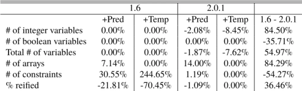
In a society where more and more production becomes automated it demands robots that are as flexible and versatile as humans. Such flexibility demands automatic scheduling of tasks. In this thesis we approach the problem using Constraint Programming and through a case study we present a model for a dual-armed robot that is able to deal with a more flexible workload. We also introduce filters to cut down the runtime of the solver. To evaluate the model we tested it on 6 solvers; G12/FD, JaCoP, Gecode, or-tools, Opturion CPX and Choco3. The results show that the model can produce a solution as good as the one manually implemented for the case study. We introduce filters on the domains of some of the variables and they made an improvement on the runtime for many of the solvers. We also found that the runtime of the solvers varied a lot and could range from several hours to just a few milliseconds using the same data. Unfortunately, in many of the tests the solvers did not complete their searches within the time limit of 4 hours. In some cases when using MiniZinc version 2.0.1, the solvers were not able to read the FlatZinc files. The fastest solver in our tests was Gecode using MiniZinc version 2.0.1.

Keywords: Constraint Programming, MiniZinc, JaCoP, G12, Gecode, or-tools, Op-turion CPX, Choco3, scheduling, dual-arm robots

Acknowledgements

I would like to thank my supervisors, Jacek Malec and Maj Stenmark, for their support and constructive feedback.

I would also like to thank Krzysztof Kuchcinski at the Institute of Computer Science, Lund University, for his valuable input on the model.

Lastly I would like to thank Johan Wessén at ABB for giving us access to the data used in [Ejenstam, 2014] and providing help interpreting the data.

Contents

2.2 Job-shop scheduling problem . . . 15

2.3 MiniZinc . . . 15 2.4 Solvers . . . 16 2.4.1 G12/FD . . . 16 2.4.2 JaCoP . . . 17 2.4.3 Gecode . . . 17 2.4.4 or-tools . . . 17 2.4.5 Opturion CPX . . . 17 2.4.6 Choco3 . . . 18 3 Case Study 19 4 Model 23 4.1 Variables . . . 24 4.1.1 Model Variables . . . 24 4.1.2 Static variables . . . 25 4.1.3 Decision variables . . . 32 4.2 Constraints . . . 33

CONTENTS 4.2.1 Precedences . . . 33 4.2.2 Predecessors . . . 36 4.3 Filter . . . 39 4.3.1 Temporal filter . . . 39 4.3.2 Predecessor filter . . . 42 4.4 Heuristics . . . 44 5 Evaluation 45 5.1 The Setup . . . 46 5.2 The results . . . 46 6 Discussion 55 6.1 Model . . . 55 6.2 Results . . . 59 7 Conclusions 61 7.1 Further work . . . 61 Bibliography 63 Appendix A Extended Model 69 A.1 Temporal filter . . . 69

A.2 Predecessor filter . . . 69

Appendix B File & Tool Manuals 73 B.1 File Formats . . . 73

B.1.1 Assembly XML . . . 73

B.1.2 Time Matrix . . . 74

B.1.3 MiniZinc data file . . . 76

B.2 AssemblyConv . . . 76

B.3 SchedPrinter . . . 76

Chapter 1

Introduction

More and more of the production in today’s society is getting automated. Product series have short lifespan and the focus of the production must change quickly. It is expensive to have at hand robots for every possible occasion, thus such production is often outsourced to low-wage countries. Often with worse working conditions than in the west. This puts pressure on the robot manufacturers to develop robots that are versatile like humans and thus eliminating the need to have multiple robots to do multiple tasks which will lower the costs and close the gap of what a human and robots are able to do.

Current robot setups usually have one robot performing one task all the time, as op-posed to flexible robots which will be changing between many different tasks and assem-blies. One of these flexible robots is ABB’s robot YuMi®. YuMi®is a dual armed robot made to work alongside humans and able to perform some of the most complex tasks, such as mount a nut or thread a needle[ABB, 2014]. It accomplishes this by using a wide variety of sensors, e.g., force sensor, visual sensors, etc. Usually a robot replaces humans to perform dangerous or heavy tasks, while YuMi®_{is mainly designed for small parts}

co-operation with humans, i.e. usually human roles in todays manufacturing environment. In order to support rapid change-over between tasks, certain problems such as schedul-ing of the assemblies need to be automated. The problem of schedulschedul-ing is a classic con-straint problem. Hence, in this thesis we will be using Concon-straint Programming (CP) to automate the scheduling process in order to cut down on the scheduling time. Constraint Programming provides a general interface to solve problems without needing to build a complete framework from scratch and makes it easy to formulate the problem through a model.

1. Introduction

1.1

Project goal

The goal of this thesis is to present a generic CP model suitable for a robot such as YuMi®, able to handle the type of jobs YuMi®is able to perform. The scope of the thesis will cover assemblies where the robot can change tools, but only being able to pick up one object at a time. Also, the change between two tools will take the same amount of time regardless whether it is from tool 1 to tool 2, or the other way around. The model will cover the use of trays, fixtures and outputs.

The model will be constructed using the MiniZinc language and tested with 6 CP solvers. We will compare the results from the solvers, both to see how well our model can perform and how well the solvers perform relative to one another.

1.2

Related work

[Drobouchevitch et al., 2006] conclude that the increasing number of machines in a robotic cell causes an explosive growth in combinatorial possibilites. They also provide evidence that a dual-gripper cell is more productive than a single-gripper cell.

[Thörnblad et al., 2013] concludes that when a cell is part of an assembly flow, the targeting of due dates instead of makespan, the total time for the assembly, is to prefer. The reason is that the focusing on makespan runs the risk of exacerbating an already unreliable flow. However, the assembly we want to construct is not a part of a flow, and thus we do not concern ourselves with maintaining a stable flow through the cell, but only to optimize the assembly in the cell.

[Yuan and Xu, 2013] states that Constraint Programming is only effective on small problems of flexible job shop scheduling. In order to effectively solve problems of larger size they suggest to use methods such as large neighbourhood search (LNS) or iterative flattening search. They also show that LNS together with Hybrid Harmonic Search pro-duces good results.

Unfortunately MiniZinc does not support the implementation of custom searches such as LNS. Therefore we try to solve the problem of ineffectiveness by using filter such as those presented by Vilím in [Vilím and Barták, 2002b] [Vilím, 2002] and

[Vilím and Barták, 2002a].

[Ejenstam, 2014] conducted a similar study also on the YuMi®_{robot. In the study}

Google or-tools was used to write the model and also implementedSystematic Tree Search,

Random Restart andLocal Searchand compared the results of using different combina-tions of them. The case study and goal of the study is different from this thesis and therefore the resulting models differ, as is discussed in chapter 6. In the study it was conclude that

Systematic Tree Search combined with Random Restart produced schedules with better results than the reference solution.

Unfortunately, not many comparisons between MiniZinc compatible solvers where found. There is an annual competition held by NICTA where solvers can compete, this is the most comprehensive documentation of the performance of the solvers we have found. Unfor-tunately, they only present which solver wins a category and no statistics are presented. Hence, no deeper comparison can be made from the result. In the latest competition held,

1.3 Report structure

2014, or-tools won three out of the four gold medals, Opturion CPX won all four silver medals and Choco won three out of the four bronze medals[NICTA, 2014c].

When presenting MiniZinc for the first time, initial tests were also presented compar-ing, amongst others, G12/FD, Gecode using FlatZinc code and native Gecode. The tests show that MiniZinc was competitive with the native Gecode model and on average the Gecode front-end for FlatZinc was about 200ms faster than the G12/FD

[Nethercote et al., 2007].

Another comparison found was [Becket et al., 2008] where they tested 10 solver on 12 problems. Unfortunately, the only solver tested there that we also used in this thesis is the G12/FD solver. So comparison with our results is hard. Although they did not draw any conclusions, G12/FD seem to fare relatively well compared to the other solvers tested.

1.3

Report structure

First we will present the approach we have taken in the thesis and present the relevant back-ground information in chapter 2. In chapter 3 we will present the case study assembly used in the thesis. Then we will present an in depth view of the model created in chapter 4. In chapter 5 we will present the setup used to evaluate the model and the result of the evalua-tion. In chapter 6 we will discuss the results and we will come to a conclusion in chapter 7. Lastly we have two appendices. Appendix A contains constraints which is not crucial for solving of the problem, but is still a part of the model. In appendix B we present all the tools used, which are free to use, and where to acquire them.

Chapter 2

Approach

2.1

Constraint Programming

Constraint programing is adeclarativeparadigm. This means that in contrast to impera-tiveparadigm languages, such as C or Java, the focus of solving problems using constraint programming is on specifying the problem and not the algorithm to solve it. However,

imperative languages, such as Java and C, can be used as a framework Constraint Pro-gramming, as in JaCoP, or-tools, and others. In Constraint Programming one specifies the

domain variables, or simply variables, andconstraints. Domain variables have domains of values, meaning they can take any value in their domain. Variables have a fixed value. Values can often be, depending on language and solver, either integers, floating-points, boolean or symbolic, symbolic being a text or label. For example a symbolic domain vari-able representing a week would have the domain

{Monday,T uesday,W ednesday,T hursday,Friday,Saturday,Sunday}, while an integer one could have{0,1,2,3,4,5,6}.

2.1.1

Constraints

Constraints are set up as relationships between the variables, and thereby limiting the do-mains of the variables. Integer dodo-mains are often used for variables, so for the rest of this section we will assume variables have integer domains. For this domain the following function symbols can be used: +,×,−and÷. The constraint relation symbols are =,<,≤,

>,≥,6=. Together with the function symbols and the constraint relation symbols, one can create simple constraint, calledprimitive constraint. An example of a primitive constraint isX < Y, i.e. the values in X’s domain has to be lower than inY’s. Primitive constraints can be used to create more complex constraints using the conjunctive connective∧. An example of this is X < Y ∧Y < 10, i.e.Y has to be less than 10 and X has to be less thanY. Since all constraints have to hold when the model is evaluated, all constraints are

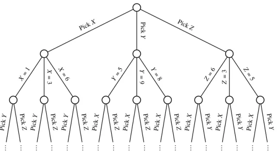
2. Approach .. . ... ... ... ... ... ... ... ... ... ... ... ... ... ... ... ... ... Pick X Pic k Y Pic k_Z X= 1 X = 3 X = 6 _Y= 5 Y = 9 Y = 8 _Z= 6 Z = 3 Z₌ 5 Pic kY Pic k Z Pic kY Pic k Z Pic kY Pic k Z Pic kX Pic k Z Pic kX Pic k Z Pic kX Pic k Z Pic kX Pic k Y Pic kX Pic k Y Pic kX Pic k Y

Figure 2.1: The beginning of the search space for the variablesX,

Y,Z, whereX ={1,3,6}Y ={5,9,8}Z ={6,3,5}

implicitly joined by a conjunction. The disjunctive connective∨is also available and can be used in the same way as∧.

For example, lets assume we have a problem with two variables,X andY,X = 4 and

Y ={1..10}. HereX has the value 4 and can thereby only take the value 4. Y on the other hand can take the values 1 to 10. This means a solution to this problem can beX = 4 and

Y = 1 or likewiseX = 4 andY = 5 , they are equally correct.

On this problem we can impose a constraint, for exampleY > X. Now we have set the constraint thatY needs to be larger thanX. And sinceX has a fixed known value we can directly see thatY > 4, since x = 4. Now with this constraint, we can reduce the domain ofY and nowY ={5..10}instead. And now a viable solution can beX = 4 andY = 7, but notX = 4 andY = 3.

2.1.2

Global constraints

Global constraints are constraints that sets up a relation between an non-fixed number of variables and the global constraints can be reduced to a set of simpler binary constraints [van Hoeve and Katriel, 2006]. They are also context independent[Beldiceanu et al., 2015], which makes them quite convenient to use when modeling and we are using a couple of global constraints that are listed below.

The description of the global constraints in this section come from MiniZinc:s global constraints listing [NICTA, 2014d] and MiniZinc:s tutorial, [Marriott and Stuckey, 2014].

All Different Constraint (

allDifferent

)

TheallDifferentconstraint is pretty straightforward. It takes a set or an arrayxas argument and enforces all variables inxto take distinctly different values, i.e. all values will be different.

2.1 Constraint Programming

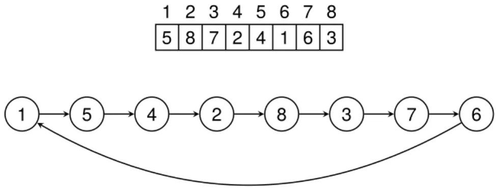
1 2 3 4 5 6 7 8 5 8 7 2 4 1 6 3

1 5 4 2 8 3 7 6

Figure 2.2: Example of the circuitconstraint enforced on an array of length 8. The visualisation of the array on top. The vi-sualisation of the nodes beneath with arrows from the node to its successor

Circuit Constraint (

circuit

)

The circuit constraint takes an array of integers representing nodes, x. Each index is representing a node and the index is the number of the node. The value at the index represents the successor of the node at the index. circuitenforces the nodes to form a

Hamiltonian circuit. This means all nodes will be part of the circuit that is formed and no node will have itself as successor. See Figure 2.2 for an example.

Cumulative Constraint (

cumulative

)

The cumulative constraint is used to schedule entities that takes a given amount of resources in a system with a known amount of resources available. The constraint takes 5 arguments; an array of start times, an array of durations, an array of resources needed and an integer for how many resources available. So if we have 5 resources available and we have two tasks which requires 3 and 2 resources respectively, they can execute simultaneously. But not if the number of available resources were 3. Each index in the arrays corresponds to an entity.

Global Cardinality constraint (

global_cardinality

)

Theglobal_cardinalityconstraint takes three arguments; an array of variablesx, an array of integercover, and an array of variablescounts. The constraint assures that the occurrences of cover(i)inxis equal tocounts(i).

2. Approach

2.1.3

Solver

A Constraint Programming program consists of many of these constraints and variables. When the problem is specified in a model, asolverruns the model. The goal of the solver is to satisfy all the constraints, i.e. set the domains of the variables so that they all follow the relationships of the constraints. This is called theconstraint satisfaction problem, and can be defined as a triple hZ,D,Ci. Z = {x₁. . .xn}is a finite set of all the variables in

the solution, D(xi), xi ∈ Z is a set representing the domain of values the variablexi can

assume, C is the set of constraints imposed on the variables inZ. In order to satisfy all constraints imposed, the solver performs a search on the space of possibilities, i.e. the

search space. The search space has the form of a tree, where each branch is a selection of a variable where the variables domain is reduced into a smaller subset that conforms with the constraints. The solver traverses the tree in search for a solution. When all variables are set to conform with the constraints a solution is found. If the solver reaches a node where a variable domain becomes empty, it has to backtrack to a previous node from which it can choose a new variable to set, i.e. traversing a new branch of that node. To make sure that all constraints holds true, called consistency, when a change occurs in a variable during search or by propagation itself, the solver performspropagation. When a change occurs to a variable, lets call it X, the solver looks at the variables related to this variable through constraints, lets call themY andZ, and may prune the domains ofY and

Zin order to uphold the consistency of the constraints. The solver then propagates onward to the variables related toY andZ and performs the same procedure. More about solvers can be found in [Tsang, 1993], [Marriott and Stuckey, 1998] and [The G12 Team, 2014].

2.1.4

Reified Constraints

Reified constraints are constraints that couple a primitive constraint with a boolean variable and provide a relationship between the both. An example could be the constraintcand a boolean variable B, the relationship between the both could bec ⇔ B. This says that ifc

holds, B=trueand if¬cholds, B= f alse. This form of expression can be very useful in expressing complex relations and constraints [Marriott and Stuckey, 1998].

Although it is a convenient way of expressing complex relations, it has its disadvan-tages. Reified constraints can be inefficient since every reified constraint needs to be prop-agated all the time. Reified constraints can also propagate poorly, for example if a variable occurs multiple times in an expression [Jefferson et al., 2010]. Due to this, we have tried to avoid direct reified constraints in the MiniZinc code in hope of reducing the total amount of reified constraints in the resulting code.

2.1.5

Branching Heuristics

Branching heuristics is what decides what value in a domain to branch on. It can be de-clared by the one programming the model and can play a significant role in the effective-ness of the model. An example of a common branching heuristic is indomain_min

which branches on the smallest value in the domain and if backtracked choses the next smallest value the next time, i.e. working its way up from the smallest value. The oppo-site of indomain_minisindomain_max, which starts in the other end of the domain.

2.2 Job-shop scheduling problem

Another common branching heuristic isindomain_medianwhich branches on the me-dian value of the domain and if backtracked branches on the values on either side of the median and works its way outwards. There are more branching heuristics available and which branching heuristics are available depend on the solver.

2.2

Job-shop scheduling problem

The job shop problem can be described as n jobs of varying size containing a number of operations to be executed in a certain order that needs to be scheduled onmidentical machines. Commonly the goal is to minimize the total time for the schedule, called the

makespan. The traveling salesman problem is a version of the job shop problem where

m= 1. [Garey et al., 1976] shows that the job shop problem is NP-complete form≥2 and

n≥3, hence more complex versions of the job shop problem will be at least this hard. As described above, the schedule is composed of jobs containing operations. This is the usual way of describing it in the literature, but we will look at it in a slightly different way. Instead of looking at many jobs, we will focus on one job and the operations within that job. In this thesis we will refer to these operations as tasks.

An extension of the job shop problem is the flexible job shop problem. In it, tasks are not locked to be scheduled on a particular machine, but can be scheduled for any of the machines [Thörnblad et al., 2013]. This increases the complexity of the problem.

Yet another extension of the job shop problem is the job shop problem with sequence-dependent setups. This means the time for a task is not just the time it takes to execute the task itself, but also the time it takes to set up the machine, depending on the previous task, in order to execute the task at hand. This is also something that increases the complexity compared to the basic job shop problem.

Our case will be a combination of the flexible job shop problem and the job shop problem with sequence-dependent setup times since, as will be described later, we can change the tools of the machines. The ability to change tools means that all machines can execute all tasks, and the change of tool takes time which means we get a sequence-dependence.

2.3

MiniZinc

There are many solvers for CP problems, but they all use different languages and as a modeler it might be of interest to test how well your model performs on different solvers. To eliminate the need to rewrite models to fit the language of the different solver in order to perform a comparison, MiniZinc was introduced. MiniZinc is a modeling language similar toOptimized Programming Language(OPL), but is scaled down and lacks some of OPL’s features. MiniZinc’s strength lies in that it is coupled with another language called FLatZinc. The difference between MiniZinc and FlatZinc is that MiniZinc is a medium-level language where it is easy for modelers to express themselves and FlatZinc is a low-level language that is easy for interpreters to parse. There is a translator from MiniZinc to

2. Approach

MiniZinc Translator FlatZinc Solver Result

Figure 2.3: The toolchain in MiniZinc

FlatZinc provided, the translation is calledflattening. MiniZinc provides a set of already defined constraints that solvers can use, however, the translator takes in consideration the solver that is going to be used and can apply custom versions of the constraints specified for that particular solver. [Nethercote et al., 2007]

Although MiniZinc aims at being a standard language in CP, it does not have support for defining custom search algorithms, as many other languages do. This means we cannot utilize algorithms for random restart, local search, etc. To be clear, the solver is the one performing the search, but in some Constraint Programming languages we can define how that search is to be performed. [Nethercote et al., 2007]

To summarise, the process of solving a problem with MiniZinc will follow the toolchain in Figure 2.3. The MiniZinc file is first passed through the translator which produces a FlatZinc file. The FlatZinc file is fed to the solver which performs the search and produces a result.

2.4

Solvers

This thesis will test the model using 6 different solvers;G12, JaCoP,Gecode, OR-tools,

Opturion CPX andChoco3. There where three requirements considered when we chose the solvers:

• The solver has to have a FlatZinc parser

• The item has to be free to acquire, either via open source, free license or free aca-demic license.

The model was initially tested during the implementation phase using G12/FD, but after a while G12/FD was unable to produce results and a switch was made to JaCoP. In other words, the model was developed and tested using JaCoP.

Which solvers implement which global constraints, or more precisely which global con-straints are used in the produced FlatZinc file, are presented in section 5.2.

2.4.1

G12/FD

G12/FD is a finite domain solver provided by the G12 team, the creators of MiniZinc. It is implemented in Mercury and is the default solver for the G12 FlatZinc interpreter [Becket et al., 2008] [NICTA, 2014c].

2.4 Solvers

2.4.2

JaCoP

JaCoP stands for Java Constraint Programming solver, and is an open source Java library for Constraint Programming that is available under the GNU Affero GPL license. It has been developed since 2001, mainly by Krzysztof Kuchcinski and Radoslaw Szymanek. The library provides many global constraints in order to make modeling more efficient. It is used by researchers all around the world and has proven its efficiency by winning silver medal in the MiniZinc Challenge [Szymanek, 2010b] [Szymanek, 2010a].

2.4.3

Gecode

Gecode is a free constraint solver under the MIT License implemented in C++. It offi-cially provide a MiniZinc interface, but many external projects provides additional inter-faces. One of its strengths is that it can perform parallel searches using multiple cores and this gives the solver great efficiency. The parallel search performs its search by having a "worker" on one core start the search. Then other "workers" on other cores can come in an "steal" a part of the search tree to work on and thereby parllelising the search. This has lead to Gecode winning all the gold medals of the MiniZinc challenge in all 5 consecutive years between 2008 and 2012. [Schulte et al., 2014]

2.4.4

or-tools

or-tools is an open source constraint solver under the Apache License 2.0 implemented in C++. or-tools is developed by Google and is part of their Operational Research. As with Gecode, or-tools also has support for parallel search. However, if this functions the same way as in Gecode is unclear. In addition to C++ and MiniZinc, or-tools also has interfaces for Python, Java and C#

[van Omme et al., 2014].

2.4.5

Opturion CPX

Opturion CPX is a constraint solver developed by Opturion Pty Ltd, a commercial outcome of the G12 project. The same ones that created G12/FD, MiniZinc and FlatZinc. Opturion CPX is a commercial product and therefore not free. Although, they provide academic licenses which was used for the thesis. Since it originated from G12, the language for implementing models is MiniZinc.

Unlike the other solvers used, Opturion CPX is not a pure finite domain solver, but rather a combination of solving techniques from CP and propositional logic (SAT). This makes CPX extremely efficient in solving large models. It is said that because Opturion CPX only generates propositional variables needed for the search, the search is not nec-essarily slowed down due to large domains. Proof of this can be shown by the number of awards claimed in the MiniZinc challange [Opturion Pty Ltd, 2013]

2. Approach

2.4.6

Choco3

Choco3 is a finite domain [Fages et al., 2014] constraint solver implemented in Java and it is free under the BSD license. The development of Choco has been going on since the early 2000s and Choco3 is the latest version. Although sharing the name, Choco3 is not the same system as its predecessor Choco2, but a complete new implementation of the previous system [Charles Prud’homme, 2014].

Chapter 3

Case Study

In order to develop and test the model, we have chosen to focus on one representative case study. In this case study the robot is assembling an enclosed emergency stop button used in industrial environments, see Figure 3.1. The assembly is presented in [Stolt et al., 2013] and has an associated video of the assembly1. Please note that this is not the video used to extract the times for the tasks, so the times may differ from the ones used. Also, only the assembly of one stop button is performed in this thesis, not several as in this video.

This assembly is composed of 5 components; a top, a button, a nut, a switch and a bottom. A combination of components that is not the complete assembly we will call a sub-assembly. The button needs to be inserted in the top and then the nut needs to be screwed onto the underside of the button in order to secure it to the top. The switch needs to be mounted in the bottom and, lastly, the top part, with button and nut, needs to be mounted on the bottom with the switch. In Figure 3.2 we see the top-button-nut assembly to the right and the bottom-switch assembly to the left. Note that the screws in the figure are not part of the case study assembly.

The assembly includes objects such as trays and fixtures. A tray is a holder where components reside until they are needed in the assembly. A fixture is a holder in which components can be put so that another components can be mounted on it.

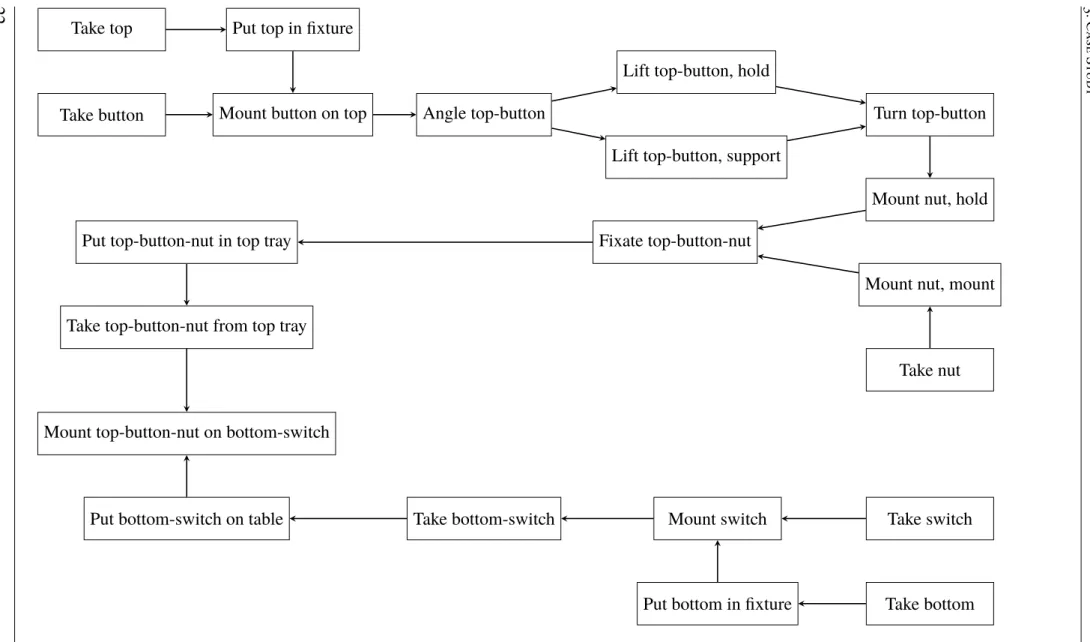
21 steps have been identified as needed for the assembly and they are taken from a video of an existing assembly created by hand. For an illustration of the order of the assembly steps, see Figure 3.2 The steps are as follows:

Take top Takes the top component from its tray

Put top in fixture Puts the taken top component in a fixture

Take button Takes the button component from its tray

3. Case Study

Figure 3.1: Picture of the button used in the case study. The screws are not part of the case study assembly

Mount button on top Mounts the taken button component onto the top component in a fixture

Angle top-button Angles the sub-assembly that is the top and button component, from here on called top-button, so it can be supported by the other machine. Although this task is called "angle", this task is a take task. So it first takes the the top-button and the angles it.

Lift top-button, hold top button Lifts the top-button by holding the button

Lift top-button, support Lifts the top-button by supporting the top from underneath

Turn top-button Turns the top-button by holding the button

Take nut Takes the nut from its tray

Mount nut on top-button, hold Mounts the nut on top-button while holding the button

Mount nut on top-button, mount Mounts the nut on the top-button holding and screw-ing the nut. The sub-assembly created by the top-button and the nut is here on after called top-button-nut

Fixate top-button-nut Fixates the top-button-nut using the side of a fixture in order to get it straight.

Put top-button-nut in top tray The top-button-nut is put in the top tray in order to put it away for a while to be picked up later.

Take top-button-nut from top tray Takes the top-button-nut from the top tray where it was previously put.

Take bottom Takes the bottom component from its tray.

Take switch Takes the switch component from its tray.

Mount switch in bottom Mounts the switch on the bottom in the fixture the bottom was put in. The sub-assembly created here will be called bottom-switch.

Take bottom-switch Takes the created bottom-switch from the fixture.

Put bottom-switch on table Puts the bottom-switch on the table.

Mount top-button-nut on bottom-switch Mounts the top-button-nut on the button-switch on the table.

Most of the steps are self explanatory, but there are a few steps which are quite special that might need some more explanation. In steps Mount nut on top-button, hold and

Mount nut on top-button, mountthe button component has been put in the hole of the top and needs to secured using the nut component. To do we utilize somthing that is special for YuMi®_{, using both arms in order to mount the nut. This is done mid air with one arm}

holding the top-button by gripping the button part, having it upside-down compared to how it was in the fixture, and with the other arm screwing the nut in place. The preparation for this starts at the end of stepMount button on top, where the sub-assembly top-button was just created, but the button is only loosely sitting in the hole of the top. The sub-assembly is angled in taskAngle top-buttonabout 45◦_{in order to create a gap under the sub-assembly}

so the other arm can reach under the sub-assembly and help lift it from the fixture in tasks

Lift top-button, supportandLift top-button, hold top button. Finally the top-button is rotated by only holding it with one arm in the button part of the sub-assembly and are now ready for the nut to be mounted. It should be noted that since the operations of lifting the top-button and mounting the nut takes two arms and we have here split the operations into two tasks each, one for each arm, the tasksMount nut on top-button, holdandMount nut on top-button, mount needs to be performed at the same time. The same goes for

Lift top-button, supportandLift top-button, hold top button.

As mentioned before, the steps listed are taken from a video of an assembly. This makes the times used in the case study approximated. First the times where approximated using seconds as the unit of time. But it showed to be hard to approximate some of the tasks as they sometimes where under 1 second. Because of this and to get better print outs of the assembly usingSchedPrinter(see appendix B) we multiplied the times we could estimate well from the video by 5 and approximated the other tasks as well as we could. This means that the real times for the tasks in the case study, and in the files mentioned in appendix B, are 1/5 of the time presented. Because of this, comparing the time from the solvers with the time of the manual assembly is harder. We had to approximate the time of the manual assembly using the times we have approximated. By analysing the video and using the approximated times we got a time of 516 time units for the manual assembly.

3. C ase S tud y

Take top Put top in fixture

Take button Mount button on top Angle top-button

Lift top-button, hold

Lift top-button, support

Turn top-button

Mount nut, hold

Mount nut, mount

Take nut Fixate top-button-nut

Put top-button-nut in top tray

Take top-button-nut from top tray

Take switch Mount switch

Take bottom Put bottom in fixture

Take bottom-switch Put bottom-switch on table

Mount top-button-nut on bottom-switch

Figure 3.2: The case study assembly

Chapter 4

Model

This model is inspired by the work in [Ejenstam, 2014]. That model is centered around work performed in fixtures. So tasks can easily be labeledtrayif it uses a tray,fixtureif it uses a fixture, etc. These are common robot in cell assembly procedures; take a compo-nent from a tray, put it in a fixture, get another compocompo-nent, mount the compocompo-nent on the the component in the fixture. But YuMi can perform much more complex tasks than that. We want to be able to schedule mounting tasks that do not incorporate a fixture. We have used a similar way of generalizing tasks by labeling them withtray,fixture, etc.

Before going into details, we will give a brief overview of how the scheduling works. The model presented is centered around tasks. A task is an action that manipulates a com-ponent in some way and is performed at a certain spacial coordinate in the room. However, the model does not care about the exact coordinates, but rather the duration it takes to travel between the coordinates. This time is used to establish how long the move from one task to the next will take. These moves are present for all tasks. If two tasks are performed at the same location, the move time will be 0. The times needs to be calculated beforehand and put in a matrix which is used to generate the input file for the model. The procedure is described in appendix B.

In the model each robot arm/manipulator is called a machine. Hence, a two-armed robot is modeled in the same way as two one-armed robots. To compensate for the place-ment of the machines there are variables that can be set as shown below. The arms can be equipped with certain tools, different tasks can require different tools and the arms can during execution change tools. The change of a tool is incorporated in the move from one task to another. This is part of what the model will try to decide, when in the assembly should we put the changes between the tools. If a change occurs between two tasks, it will be shown by the move time being extended with the duration of a tool change. To both know how long the move between two tasks will be and if there needs to be a tool change, we need to know which task comes before another task, i.e. the predecessor.

4. Model

The goal of the assembly is to assemble components into sub-assemblies and further into a final assembly. All the intermediate assemblies before the final assembly are called sub-assemblies. For reasons explained further down, we will in this thesis call components fed from the outside into the assembly, such as buttons, for primitvecomponents instead of just components.

The tools used to generate the data used in this thesis are free to use and are described in appendix B. The complete model file used can be found athttps://github.com/ Arclights/Thesis-ToolsunderData.

4.1

Variables

The solver takes a description of the robot cell in the form of a MiniZinc data file. The file describes the number of available arms, tools, trays, fixtures etc. The variables provided by the data file are calledmodel variablesand they will be explained further down among the

static variablestogether with some additional variables created using themodel variables.

4.1.1

Model Variables

4.1 Variables

task task task task sTask1 sTask2 gTask1 gTask2

Figure 4.1: An example of the tasks and start and goal tasks seen as an array for an assembly with 4 tasks and 2 machines

• timeMatrixDepth

• timeMatrix3D(t1, t2,k) • tasksOutO f Range(t)

4.1.2

Static variables

Static variables are variables that have a fixed value, or is a set or list containing fixed values.

First we define the number of tasks to be scheduled. Each task is identified by a num-ber from 1 tonbrT asks.

nbrT asks∈ {1, . . . ,232−1} (4.1)

tasks={1, . . . ,nbrT asks} (4.2) Here we define the machines available for the assembly. A machine in this model is an arm.

nbrMachines∈ {1, . . . ,232−1} (4.3)

machines={1, . . . ,nbrMachines} (4.4) As mentioned, this model is based on the technique of using predecessors to determine which task comes directly before another. This creates the need to have source and a sink node for each machine. We call them start tasks and goal tasks. As they are not provided as parameters, the model creates them and give them identifiers with numbers greater than the tasks to be scheduled. Each machine has to have a start task and a goal task. This means that there are as many start and goal tasks as there are machines. They are arranged so that all the start tasks come first and then all the goal tasks. One can easily find the start task for a machine bynbrT asks+m, where mis the machine in question. It is also easy to find the matching goal task bynbrT ask+m+nbrMachines. If one thinks of the tasks, start and goal tasks as an array where the index is the number of the task, then it would look like in Figure 4.1.

startT asks={nbrT asks+ 1, . . . ,nbrT asks+nbrMachines} (4.5)

goalT asks={nbrT asks+nbrMachines+ 1, . . . ,nbrT asks+nbrMachines×2} (4.6) We group together all tasks in one set in order for a more readable notation further down.

allT asks=tasks∪startT asks∪goalT asks (4.7) These are the tools that can be fitted on an arm. The model assumes that there is a set of

nbrT oolsfor each machine. I.e. if nbrT ools = 2 andnbrMachines = 2, there is a set of tool 1 and tool 2 for machine 1, and another set of tools 1 and 2 for machine 2. There

4. Model

cannot be a combination of tools such as, for example, only tool 1 for machine 1 and a set of tools 1 and 2 for machine 2.

toolNeeded(t) defines the tool that tasktneeds.

nbrT ools∈ {1, . . . ,232−1} (4.8)

tools={1, . . . ,nbrT ools} (4.9)

toolNeeded(t)∈tools, t ∈tasks (4.10)

nbrComponents defines the number of components used. All components need to be uniquely identified in the assembly, so even if we use 4 identical screws in an assembly, we need to define all 4 screws. As mentioned before, we distinguish between components andprimitve components. The reason for this is that in the model we do not distinguish between aprimitvecomponent and a sub-assembly, they are the same. And in the model we call them components. The reason for this is because we found it easier to only have one sort of object to deal with when it comes to what will be assembled, instead of two. This means that the final assembly is also a component, i.e. the product produced by the assembly is a component. In other words, in this thesis primitve components and sub-assemblies are sub sets of components.

componentsUsed(t) defines the set of components task t uses. A task usually only uses one component at a time, but uses two in the case of mounting tasks, the mounted component and the component mounted on.

To know when a sub-assembly is created we set it ascompoentCreated for the task where it is created. This cannot happen anywhere else than in a mount task, although there is no check in the model for it. If no component is created in a task,componentCreated = 0.

nbrComponents∈ {1, . . . ,232−1} (4.11)

components={1, . . . ,nbrComponents} (4.12)

componentsUsed(t)⊂ components, t ∈tasks (4.13)

componentCreated(t)∈components∪ {0}, t ∈tasks (4.14) Since components also can be sub-assemblies, it means a component can have subcompo-nents. These have been grouped in different groups to assist the constraints.

taskSubComponents(t) is the set of components that make up the subcomponents for the components used in task t. One can think of the subcomponents as layers with the component on top, call it origin component, and the layer below are the components that make up that component, and so on. taskSubComponents(t) contains the compo-nents one layer down, if the component itself is not a primitvecomponent. In that case,

taskSubComponents(t) contains that component instead. See Figure 4.2 for an example.

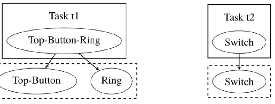
taskSubComponents(t)⊂components, t ∈tasks (4.15) To use the layer metaphor again,taskCompleteSubComponents(t) contains all the layers below the origin component, for all the components in task t, not including the origin component itself. If the origin component is aprimitvecomponent, the set is empty. See Figure 4.3 for an example.

4.1 Variables Task t1 Top-Button-Ring Top-Button Ring Task t2 Switch Switch

Figure 4.2: taskSubComponentsfor two tasks,t1 andt2. t1 con-tains a sub-assembly, Top-Button-Nut, and t2 contains a primi-tive component, Switch. ThetaskSubComponents for each task is shown in the dashed box beneath them.

Task t1 Top-Button-Ring Top-Button Top Button Ring Task t2 Switch

Figure 4.3: taskCompleteSubComponents for two tasks, t1 and t2. One contains a sub-assembly, Top-Button-Nut, and the other contains a primitive component, Switch. The

taskCompleteSubComponents for each task is shown in the dashed box beneath them.

4. Model

subComponents(c) contains only the the primitve subcomponents for componentc, one layer down. If c is a primitve component or is only made of sub-assemblies, the set is empty.

subComponents(c)⊂components, c∈components (4.17) Trays are used to hold components until we need them in the assembly. It can be that the tray holds the components from the beginning, as with primitve components fed to the assembly, or it can be a sub-assembly put there during the assembly to be picked up again later. Eachprimitvecomponent has its own tray, so we can have a button tray, a cover tray, etc.

tray(t) is the tray tasktuses. If no tray is used by the task,tray(t) = 0.

nbrTrays∈ {1, . . . ,232−1} (4.18)

trays={1, . . . ,nbrTrays} (4.19)

tray(t)∈trays∪ {0}, t ∈tasks (4.20)

f ixturesdefines the fixtures available in the assembly. A fixture is primarily used to hold a component in order for another component to be mounted on that component. Although, as was shown in the case study in chapter 3, the fixture can be used for purposes other than just holding components.

f ixture(t) is the fixture tasktuses. If no fixture is used by the task, f ixture(t) = 0

nbrFixtures∈ {1, . . . ,232−1} (4.21)

f ixtures={1, . . . ,nbrFixtures} (4.22)

f ixture(t)∈ f ixtures∪ {0}, t ∈tasks (4.23)

out putsdefines the outputs available. An output is the final stage for a component in an assembly. After it is put here, it will not be removed. Although, there can still be other components mounted on the component put on the output. In that respect an output can be viewed as a fixture, only that the components put there can not be removed.

out put(t) is the output used by taskt. If no output is used by the task,out put(t) = 0.

nbrOut puts∈ {1, . . . ,232−1} (4.24)

out puts={1, . . . ,nbrOut puts} (4.25)

out put(t)∈out puts∪ {0}, t ∈tasks (4.26)

concurrentT asks(k) is thek:th concurrent group among the concurrent groups defined. A concurrent group is a group of tasks that has to be performed at the same time. Hence, a concurrent group can not be larger than the amount of machines available, although, there is no check for it in the model.

nbrConcurrentGroups∈ {1, . . . ,232−1} (4.27)

concurrentGroups={1, . . . ,nbrConcurrentGroups} (4.28)

4.1 Variables

orderedGroup(k) is thek:th ordered group specified, there are nbrOrderedGroups or-dered groups. An oror-dered group is an array of tasks that have to come in a very specific order. An example of this could be if an assembly has many move tasks that need to be performed one after another in order to make some intricate movement. As seen in section 4.2, we can reason about the relation between tasks if they use a certain component and are a certain kind of action. But we cannot reason about two move tasks, there is no way to tell which should come before the other based on the component they use.

orderedGroup(k) is an array and the tasks in it will be scheduled in the order they come in the array. All the tasks in the group will be performed on the same machine.

If one wants to access a certain task in a group, one can useordered(k,i) to access the

i:th element of thek:th group.

orderedSet is the set of all tasks included in some ordered group.

nbrOrderedGroups∈ {1, . . . ,232−1} (4.30)

orderedGroups ={1, . . . ,nbrOrderedGroups} (4.31)

orderedGroup(k)⊂ tasks, k ∈orderedGroups (4.32)

ordered(k,i)∈tasks, i∈ {1, . . . ,|orderedGroup(k)|}, k ∈orderedGroups (4.33)

orderedSet = [

∀k∈orderedGroups

orderedGroup(k), orderedSet ⊂tasks (4.34)

tray(t),out put(t) and f ixture(t) cannot be set at the same time for a task, since that would mean that the task is performed at two locations at the same time, although this is not checked by the model. The only restriction for what kind of tasks can be performed using these containers is that outputs cannot be used by take tasks and trays cannot be used by a mount tasks. If an assembly contains these combinations, the output or tray should be changed to a fixture.

Each task performed can be classified as either a mount task, a take task, a move task or a put task, but only as one of them.

Taking A task that picks up a component is a taking task. The location of the component is specified by either a tray or a fixture, but not an output since there is no reason to pick up something that has been placed on an output.

Mounting A task that mounts a component on another component is a mounting task. This assumes that the component to mount is picked up and in the hand. The location of the component to mount on is defined by either a fixture or an output.

Putting A task that puts a component somewhere is a putting task. Where a component is put is defined by either a fixture, a tray or an output.

Moving A task that moves a component from one place to another is a moving task. The model already puts in moves between tasks and if, for example, the first task is a take task and the second task is a put task, the move in between them is essentially a move that moves a component from one place to the another. Although, sometimes it can be handy to define a task that explicitly moves a component. An example of that can be if one wants to spin a component around. Then one can specify a take task in order to pick up the component, a move task to turn it, and a put task to put

4. Model 9 7 1 2 4 8 5 3 6 1 8 9 8 1 5 6 2 4

9

7

1

5

6

8

2

3

9

Figure 4.4: The timeMatrix3D

the component back. In this case there will be three moves of the component; one to move from the take task to the move task, the move task itself, and a move from the move task to the put task.

mounting⊂ tasks (4.35)

taking⊂ tasks (4.36)

moving⊂tasks (4.37)

putting⊂tasks (4.38)

putting(c),mounting(c),taking(c) andmoving(c) are subsets of respective set above based on the component involved.

putting(c) ={t :t ∈ putting, c∈componentsUsed(t)}, c ∈components (4.39)

mounting(c) ={t :t ∈mounting, c∈componentsUsed(t)}, c∈components (4.40)

taking(c ={t :t ∈taking, c∈componentsUsed(t)}, c∈components (4.41)

moving(c) ={t :t ∈moving, c∈componentsUsed(t)}, c∈components (4.42)

duration(t) is simply the duration of taskt.

duration(t)∈ {0, . . . ,232−1}, t ∈tasks (4.43) For the model to decide how long a move between two tasks should take and whether there should be a change of tool in between, a matrix is used, timeMatrix3D, see Figure 4.4. This is a 3-dimensional matrix and contains the times for moving between all the tasks depending on what tool change occurs. On its y-axis it has the tasks to move from, on the x-axis the tasks to move to, and on the z-axis the different transitions between tools that can occur. There are nbrMachines more rows on the y-axis than there are columns on the x-axis. This is because we also account for the starting position of the machines, so each start task has move times associated with them for moving to the other tasks. As the matrix is constructed the way it is, there is no move times between start tasks.

4.1 Variables 1 2 3 1 2 3 1 2 3 1 2 3

Figure 4.5: All the transitions between the tool states to the left. The reduced number of transitions between the tool states to the right

timeMatrixDepth is the length of the z-axis, i.e. the depth of the matrix. It should be said that the reason for using the method described below is to reduce the size of the matrix and avoid redundancy.

What we mean with ”different transitions” is easiest shown through an example. Let us say we have 3 tools available for each machine. We consider each tool state as a node in a graph, see Figure 4.5, with the old tool state to the left and the new tool state to the right. Between them we can draw the different ways we can change state. The we start to consider which ones we actually need. We can change from tool 1 to tool 1, which is not changing tool at all. The same can be done for tool 2, but not changing tool here costs just as much time as with tool 1. So the change from tool 1 to itself covers not changing tool for this tool, as well as for all the other tools, thereby we only need to keep track of one of these changes. We can also change from tool 1 to tool 2. And we can change back from 2 to 1, although here in the model we assume the change from one tool to another takes the same time the other way around as well. Therefore, we consider the change from tool 1 to tool 2 the same as from tool 2 to tool 1, and only keep track of one of them. If we keep considering the rest of the transitions this way, we will end up with a reduced number of transitions, in our case 4, see Figure 4.5

It is clear that,timeMatrixDepthobeys the equation (4.44).

timeMatrixDepth= n

2_{−n+ 2}

2 , n= nbrT ools (4.44)

timeMatrix3D(t(f rom),t(to),k)∈ {0, . . . ,232−1}, t(f rom)∈tasks∪startT asks,

t(to)∈tasks, k ∈ {0, . . . ,timeMatrixDepth}

(4.45)

Depending on the physical layout of the assembly, sometimes not all the tasks can be done by all machines. It could be that the machines would collide or simply that the spatial location is out of reach for the machine. In those cases we can specify that tasks are out of hand for a specific machine. This is the only time when we distinguish between the two machines and connect the machine in the model model with the machine in the real world. In all other aspects the machines in the model are identical and have the potential to perform the same work.

4. Model

4.1.3

Decision variables

Decision variables are variables that can take many values. It is these values that the solver sets out to determine in order to solve the problem.

The model has to decide which task uses which machine.

usingMachine(t)∈machines, t∈tasks (4.47) Each task has a predecessor that tells the model what other task comes right before the task in question on the same machine.

pred(t)∈allT asks, t ∈allT asks (4.48) In order to create an upper limit for variables dealing with time, we create a rough upper limit of the complete assembly. It simply takes the longest duration for a task and the longest duration for a move between tasks and assert it for all the tasks.

maxE= (max({duration(t) :t∈tasks}) +

max({timeMatrix3D(t1,t2,k) :

∀t1∈tasks∪startT asks,

∀t2∈tasks,

∀k∈ {0, . . . ,timeMatrixDepth}})×nbrT asks

(4.49)

Each task has to have a start time. We set it to be anywhere between time 0 and the maximum possible end calculated before.

To simplify notation we also introduce one more variable calledend(t). It is the time when tasktends and is simply the sum of the start and the duration of the task.

start(t)∈ {0, . . . ,maxE}, t ∈allT asks (4.50)

end(t) =start(t) +duration(t), t ∈allT asks (4.51) As mentioned before, each task has a move time connected to it since it takes a certain amount of time to move from one task to another. Since this time depends on both what task comes before it and what tools are needed for both of the tasks, the duration for the move is a decision variable as opposed to the duration for the task itself.

moveDuration(t)∈ {0, . . . ,maxE}, t∈allT asks (4.52)

moveStart(t)∈ {0, . . . ,maxE}, t ∈allT asks (4.53)

moveEnd(t) =moveStart(t) +moveDuration(t), t ∈allT asks (4.54) Since the goal of the assembly is to complete the assembly in as little time as possible, we set up a variable for it,makespan. It is this variable the solver will try to minimize.

makespan∈ {0, . . . ,maxE} (4.55) The last variable is for determine what tool should be used for a task. WithtoolNeeded

we specify what tool is needed for the specific task. But we do not need to specify a tool if the task does not need any specific tool. That is why we need to determine what tool should be used for those tasks. Leaving the option open by not specifying any particular tool opens up for optimisations since it could mean we can avoid costly tool changes.

4.2 Constraints

4.2

Constraints

In this section some of the most important constraints for the model will be described. For a full list of used constraints seeAppendix A, while for the MiniZinc code seeAppendix B.

makespan should represent the total time of the whole assembly. That means it should be equal to the largest end time among all the tasks. We can enforce that by limiting the end time for each task to be less or equal to themakespan.

(∀t ∈tasks)end(t)≤makespan (4.57) Start and goal tasks are special tasks since they act as source and sink nodes. This means they never get scheduled in time as ordinary tasks, we set them to all start at time 0 and they do not have a duration variable, since they do not take up any time. We also assign them to machines so each start and goal task pair have their own machine from the start.

(∀t ∈startT asks∪goalT asks)start(t) = 0 (4.58) (∀m∈machines)usingMachine(nbrT asks+m) =m

∧usingMachine(nbrT asks+nbrMachines+m) =m (4.59)

We enforce thetasksOutO f Range(m) variables by simply saying that the tasks in the vari-able can not be assigned the machinem.

(∀m∈machines) (∀t ∈tasksOutO f Range(m))usingMachine(t)6=m (4.60) As said before, thetoolNeededcontains what tool is needed for a task. We need to translate it into what tool is used. It is done by simply taking the value from toolNeeded and assigning it totoolUsedfor the tasks where a tool is specified, i.e. toolNeededis not 0.

(∀t ∈tasks, toolNeeded(t)= 0)6 toolUsed(t) =toolNeeded(t) (4.61)

4.2.1

Precedences

These constraints deals with the order in time in which the tasks have to come.

A very fundamental part of the relation between a task and the move to it is that we cannot start a task before we have moved to it.

(∀t ∈tasks)Start(t)≥moveEnd(t) (4.62) If we want to mount two components together, we first have to put the first component in a fixture before we can mount the other component on it. Hence, the put task has to end before we can start with the mount task.

(∀comp ∈components) (∀mountT ask ∈mounting(comp))

(∀putT ask ∈ putting(comp))

end(putT ask)≤moveStart(mountT ask)

4. Model

In the case mentioned above we also have take tasks for both components and they must both be performed before we can start mounting anything.

(∀comp∈components) (∀mountT ask∈mounting(comp)),

(∀takeT ask ∈taking(comp)),

end(takeT ask)≤ moveStart(mountT ask)

(4.64)

Say we want to put a component away for a while and pick it up again later. Then we need to do that in a tray. This is the only time we put anything in a tray, usually we just take components from them. So we can apply the (4.65) constraint which says that if there is a take and a put on the same tray, then the take has to happen after the put.

(∀comp ∈components)

(∀putT ask ∈ putting(comp), tray(putT ask)> 0)

(∀takeT ask ∈taking(comp), tray(putT ask) =tray(takeT ask))

end(putT ask)≤moveStart(takeT ask)

(4.65)

When there is a put task and a take task on a fixture where a sub-component of the com-ponent being taken is the comcom-ponent being put, the put task has to happen before the take task.

(∀f ∈ f ixtures)

(∀putT ask∈ putting, f ixture(putT ask) = f) (∀takeT ask ∈taking, f ixture(takeT ask) = f ∧

componentsUsed(putT ask)⊂taskSubComponents(takeT ask))

end(putT ask)≤ moveStart(takeT ask),

(4.66)

Since we can do many sub-assemblies on the same fixture, we need to ensure that if a component is put in the fixture, there cannot be a component from another sub-assembly put or mounted there before the sub-assembly is done.

We can observe that the task of doing a sub-assembly begins with a put of a component in a fixture and a take of a component from the same fixture. The taken component will have the put component as a sub-component. With this knowledge we start by extracting all put tasks for a fixture. Then we extract all the corresponding take tasks, i.e. the take tasks for that fixture where the component used in the put task is among the sub-components for the component in the take task. Although, there is the case where we construct a component by first doing some mounting, then we take it up to maybe turn it or fixate it, and then put it back in the fixture for further mounting. In this case we will get two takes matching with the first put. So we need to identify which take task is the first one. We do this by choosing the take task with the least amount of subcomponents.

Now we have a 1:1 matching of take tasks and put tasks. To ensure the time between when a put task occurs and when the take task occurs, we apply acumulative constraint over that time and the limit of the fixture is always 1.

When [ and ] are used together with : as below, it means they are array generators. What is left of the : is what is put in the array and what is right of it is the condition. A

4.2 Constraints

case here which might be confusing is the last argument to the cumulative constraint. It simply states that it is an array of ones with the same length as puts.

(∀f ∈ f ixtures)

puts= [put: put ∈ putting, f ixture(put) = f],

takes= [min({take:take∈taking, f ixture(take) = f,

componentsUsed(put)⊂taskCompleteSubComponent(take)}) :

put∈ puts],

cumulative([moveStart(task) :task ∈ puts],

[abs(end(takes(i))−moveStart(puts(i))) :i∈ {1, . . . ,|puts|}], [1 :i ∈ {1, . . . ,|puts|}],

1)

(4.67) The fundamental property of the tasks in a concurrent group is that they need to execute at the same time on different machines. We ensure this with (4.68).

(∀group∈ {1, . . . ,nbrConcurrentGroups}) (∀t1 ∈concurrentT asks(group))

(∀t2 ∈concurrentT asks(group)\ {t1})

start(t1) =start(t2)∧

usingMachine(t₁)6=usingMachine(t₂),

(4.68)

A very logical observation we can do is that components cannot be used before they are created. This is enforced in (4.69).

(∀t1 ∈tasks, componentCreated(t1)> 0)

(∀t2 ∈tasks, componentCreated(t1)∈componentUsed(t2))

moveStart(t2)≥end(t1)

(4.69)

A similar observation as for (4.69) is that we have to perform all tasks with a component before it is part of a sub-assembly. Therefore we can say that all tasks need to have an end time smaller than the start time of the tasks having the tasks component as sub-component.

(∀precT ask∈tasks)

(∀t ∈tasks, precT ask 6=t,

componentUsed(precT ask)∪taskCompleteSubComponents(t)

⊂taskCompleteSubComponents(t),

componentsUsed(precT ask)∪taskCompleteSubComponents(t)6=∅)

end(precT ask)≤moveStart(t),

(4.70) Trays, fixtures and outputs can only be used one at a time. We can rephrase this into saying that tasks using trays cannot overlap, tasks using fixtures cannot overlap, etc. We ensure

4. Model

this by applying thecumulativeconstraint through (4.71), (4.72) and (4.73). (∀f ∈ f ixtures)

f ixtureT asks= [t :t ∈tasks, f ixture(t) = f],

cumulative([start(t) :t ∈ f ixtureT asks], [duration(t) :t ∈ f ixtureT asks], [1 :t ∈ f ixtureT asks],

1)

(4.71)

(∀tr ∈trays)

trayT asks= [t :t ∈tasks, tray(t) =tr],

cumulative([start(t) :t ∈trayT asks], [duration(t) :t ∈trayT asks], [1 :t ∈trayT asks],

1)

(4.72)

(∀o∈out puts)

out putT asks= [t :t ∈tasks, out put(t) =o],

cumulative([start(t) :t ∈out putT asks], [duration(t) :t ∈out putT asks], [1 :t∈out putT asks],

1)

(4.73)

4.2.2

Predecessors

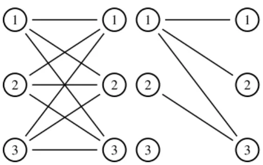
All tasks need to have a predecessor that tells the model what task comes directly before it on the same machine. This means that a task can only have one predecessor. It can be seen as the way a machine needs to travel through its tasks in order to complete the assembly, where we have a start task at the start and a goal task at the end. If we were to connect the start and the goal task we wold have a circuit, hence we could view each machine as a circuit. And we could model each machine as a circuit, but then we would need to synchronise all the sub-circuits and ensure that tasks only appeared in one sub-circuit. This would make for quite a few constraints and would make the model more complex. Instead we model all the machines as one circuit and we tie together the goal task of one sub-circuit with the start task of the next for each sub-circuit, to form a large circuit. Then we tie together the goal task of the last sub-circuit with the start task of the first, see (4.75). Lastly we can apply thecircuitconstraint over all pred variables.

The attentive reader might have observed that the nodes in thecircuit constraint have successors and not predecessors. Even if it is the wrong way around, it does not matter if the constraint sees the predecessor variable as a successor or a predecessor, it will form a circuit anyway.

(∀startT ask ∈startT asks\ {nbrT asks+ 1})