Editors: Will be set by the publisher
ON SOME RECENT ADVANCES ON HIGH DIMENSIONAL BAYESIAN
STATISTICS
Nicolas Chopin
1, S´
ebastien Gadat
2, Benjamin Guedj
3, Arnaud Guyader
4and
Elodie Vernet
5Abstract. This paper proposes to review some recent developments in Bayesian statistics for high dimensional data. After giving some brief motivations in a short introduction, we describe new ad-vances in the understanding of Bayes posterior computation as well as theoretical contributions in non parametric and high dimensional Bayesian approaches. From an applied point of view, we describe the so-called SQMC particle method to compute posterior Bayesian law, and provide a nonparametric analysis of the widespread ABC method. On the theoretical side, we describe some recent advances in Bayesian consistency for a nonparametric hidden Markov model as well as new PAC-Bayesian results for different models of high dimensional regression.
R´esum´e. Cet article propose une vue d’ensemble de r´ecents d´eveloppements en statistiques Bay´esiennes en grande dimension. Apr`es quelques motivations rappel´ees en introduction, nous pr´esentons des avanc´ees `a la fois algorithmiques et dans la compr´ehension th´eorique de m´ethodes de calculs d’a poste-riori Bay´esien. En particulier, nous d´ecrivons l’algorithme particulaire SQMC et proposons un point de vue non-param´etrique de la m´ethode populaire ABC. Nous revenons ensuite ´egalement sur des nouvelles contributions en statistiques bay´esiennes non param´etriques et en grandes dimensions. Dans ce contexte, nous d´ecrivons des r´esultats de consistance bay´esienne a posteriori pour des mod`eles non-param´etriques de Markov cach´es ainsi que des r´esultats PAC-bay´esiens pour diff´erents mod`eles de r´egression.
1.
Introduction
The analysis of Bayesian methods for high dimensional and non parametric models are at the cornerstone of some new statistical developments. Bayesian methods are tempting owing to their great generality and ability to incorporate in the statistical approach a belief of what should be the unknown quantity to be estimated (for example). It is also useful for producing efficient estimators or confidence set. It has recently attracted a lot of attention thanks to the availability of massive computational resources: in the 2000s, Bayesian works have been developed to deal with very high dimensional or even non parametric problems. This evolution also guided by very concrete applications in biostatistics and signal processing (among others) has raised new natural questions that mainly concern two important points. The first one asks how should be a “good” Bayesian prior
1 ENSAE, 3 Avenue Pierre Larousse, 92245 Malakoff, France
2 Toulouse School of Economics (Universit´e Toulouse I Capitole), 21 all´ees de Brienne, 31000 Toulouse, France 3 Modal project-team, Inria Lille - Nord Europe. 40 avenue du Halley, 59650 Villeneuve dAscq
4 LSTA, Universit´e Pierre et Marie Curie & Projet ASPI, INRIA Rennes, France 5 Universit´e Paris-Sud, 91405 Orsay Cedex France
c
for high dimensional or non parametric statistical model and what kind of theoretical results on the posterior distribution could we expect when the number of observations increases? The second imperative question is how to produce efficient algorithms to make it possible the computation of the posterior distribution and, if possible, quantify the way these numerical methods approximate this posterior distribution.
1.1.
Bayes approaches
In what follows, we will consider a dominated model parameterized by a set of measurable parametersΘ. We will assume thatΘis included in a metric space and each parameterθ∈Θdefines a conditional probability distributionP(.|θ). As a dominated model, all the previous lawsP(.|θ) are absolutely continuous with respect
to a common measure denotedλ, whose density will be referred to asf(.|θ).
A Bayesian prior π on Θ is an initial distribution on Θ that traduces a belief on the distribution of an unobserved parameter θ living on Θ. We are then interested in statistical inference on Θ (or in a quantity related to a distribution on Θ) when observing an i.i.d. sample of size n, denoted yn := (Y1, . . . , Yn) in the sequel. A key ingredient for the analysis of the Bayesian procedures is the likelihood ratio of the sample, written as `(yn|θ) that satisfiesP(dyn|θ) =`(yn|θ)λ(dyn). This likelihood ratio is important since it permits, at least from a mathematical point of view, to compute theposterior distribution built using theprior distribution and the famous Bayes’ rule:
π(θ|yn) = R π(θ)`(yn|θ)
Θπ(ϑ)`(yn|ϑ)dϑ
. (1)
We will see in the sequel some very nice results about the behaviour of the posterior distribution, which thus permit to compute certain quantities (e.g. mean or moments) of the posterior distribution and therefore to perform Bayesian inference.
1.2.
Posterior computation
1.2.1. Bayesian inferenceIn order to obtain a Bayesian estimator generically given by E[ϕ(θ)|yn], the standard approach is to do a
Monte Carlo procedure to roughly approach the former expectation: one simulates several independent values
θk ∼π(θ|yn), makingkvarying between 1 and K, and compute the empirical averages, e.g.
1 K K X k=1 ϕ(θk)
as an approximation ofE[ϕ(θ)|yn] =Rθϕ(θ)π(θ|yn)dθ.
A practical difficulty with this approach is that it relies on the approximation of the posterior distribution, and in most cases the denominator in (1) is an intractable integral. Fortunately, standard MCMC (Markov chain Monte Carlo) algorithms used to simulate fromπ(θ|yn) require evaluating the posterior densityonly up to a constant, and therefore do not require to evaluate this intractable integral. For instance, Algorithm 1 describes one step of a Gaussian Random Walk Hastings-Metropolis (RWHM) algorithm, that is, an algorithm for simulating a Markov chain that leaves invariantπ(θ|yn), using the following proposal mechanism (assuming Θ =Rd): from a current pointθk, propose new pointθ?∼N(θk,Σ), (a random walk move), and accept/reject
according to (informally) how more compatible is the proposed point to the posterior, relative to the current point. One sees that Algorithm 1 does not require evaluating the denominator of (1).
Algorithm 1 is just a simple example of possible practical approaches to Bayesian computation and various methods exist for the inference ofθ0in this context, such as rejection algorithms [Rip06], Markov Chain Monte
Carlo (mcmc) methods (e.g., the Metropolis-Hastings algorithm [MRR+53, Has70]), and Importance Sampling
[Rip06]. For a comprehensive introduction to the domain, the reader is referred to the monographs [RC04] and [MR07]. However, in some contexts, computation of the posterior is problematic, either because the size
Algorithm 1(Gaussian) Random Walk Hastings-Metropolis (RWHM) algorithm Input: θk, Σ (resp. a point inRd, and ad×dsymmetric positive matrix) Output: θk+1 (a vector inRd).
1: Simulateθ?∼N(θk,Σ). 2: With probability 1∧rwhere
r= π(θ ?)`(y
n|θ?)
π(θk)`(yn|θk)
take θk+1=θ?; otherwise keep the parameter unchanged: θk+1=θk.
of the data makes the calculation computationally intractable, or because calculation is impossible when using realistic models for how the data arises. Thus, despite their power and flexibility, mcmcprocedures and their variants may prove irrelevant in a growing number of contemporary applications involving very large dimensions or complicated models. This computational burden typically arises in fields such as ecology, population genetics and image analysis, just to name a few.
1.2.2. Limitations of standard RWHM
A miminal requirement to apply Algorithm 1 (and many other similar methods) is the possibility to evaluate the likelihood `(yn|θ) for any θ ∈ Θ. Unfortunately, there are various important cases where the likelihood itself cannot be exactly computed :
(1) Because the likelihood is an intractable integral: `(yn|θ) =R`(x,yn|θ) dx. Typically, xis interpreted as a latent variable in this formulation. Examples include hidden Markov models (also covered in Section 3), phylogenetic models (wherex is a phylogeny tree, seee.g.[Bea10]), and more generally any model based on latent variables.
(2) Because the likelihood isun-normalised: `(yn|θ) = gθ(yn)/Z(θ), with Z(θ) =
R
θgθ(yn 0) dy
n0 being intractable. Examples include Ising models, networks models [Eve12, CF13], models for point processes [GZ01], among others.
1.2.3. Approximate Bayesian Computation methods
Another pathological situation occurs when the model is so complicated that the only task we can perform is to sample from it. This type of problem (originally arising in genetics) has motivated a drive to more approximate approaches, in particular the field of Approximate Bayesian Computation (abcfor short).
In a nutshell,abcis a family of computational techniques that offers an almost automated solution in sit-uations where a systematic evaluation of the likelihood is computationally prohibitive, or whenever suitable likelihoods are not available. The approach was originally mentioned, but not analyzed, in [Rub84]. It was further developed in population genetics in [FL97, TBGD97, PSPLF99, BZB02], who gave the name of Approx-imate Bayesian Computation to a family of likelihood-free inference methods. Since its original developments, theabcparadigm has successfully been applied to various scientific areas, ranging from archaeological science and ecology to epidemiology, stereology and protein network analysis. There are too many references to be included here, but the recent survey [MPRR12] offers both a historical and a technical review of the domain.
1.3.
Consistency of Bayesian procedures
1.3.1. Frequentist point of view
As already discussed above, the choice of the prior is a key issue in Bayesian statistics. It can be important for computational reasons since it may help a lot to use some particular conjugate prior/posterior to accelerate the evaluation of Bayes estimators (seee.g.[GCSR04]). It is also at the core of Bayesian consistency by adopting a frequentist point of view. A natural question is the impact of the prior πon the posteriorπ(·|yn). That is to say, does the prior still play a role in the posterior when the number of observations increases or does it
“disappear” in favor of the observations? If another prior is chosen, will the posterior be approximately the same at least when the number of observations is infinite? An answer to this question is given by the concept of posterior consistency. Studying posterior consistency implies taking a frequentist point of view, assuming that the observations come from a real parameterθ0∈Θ,i.e.
yn= (Y1, . . . , Yn) are distributed fromP(.|θ0)
and wondering if the posterior concentrates its mass around θ0 when the number of observations increases
(meaning thatn−→+∞).
Definition 1.1 (Consistency). The posteriorπ(·|yn) is consistent atθ0 if for all neighborhoodU ofθ0:
P(.|θ0)-a.s., π(U|yn)−→1 as n−→+∞.
Posterior consistency may be seen as a frequentist validation of Bayesian statistics. It also ensures robustness of the posterior considering two different priors see [GR03].
The first historical answer to such a type of question is given by [Doo49]: in a very general setting, when the observations are i.i.d. and the model is identifiable, the posterior is consistent at π-almost everyθ0. The
exact set of true parameters at which the posterior is consistent is not specified in this theorem and it may be topologically small. In particular, [Fre65] proved that in the nonparametric case, the couples (π,θ0) for which
the posterior is consistent is very small topologically (meager). This negative result is not a reason to give up nonparametric or high dimensional Bayesian statistics: on the contrary it is a clear invitation to a careful choice of a good prior to resolve a given statistical problem.
A general and now usual method to prove consistency was introduced by [Sch65]. Some historical modifica-tions can also be found in [IH81] but recent advances stand on the seminal work of [Bar88]. Roughly speaking, Bayesian consistency holds if the prior puts some mass on any closed neighborhood of θ0 and if there exist
exponentially consistent tests to discriminate θ0 against the complementary of all neighborhood of θ0(for the
considered topology) intersected with a set with an exponential decreasing prior mass. An important under-lying concept resides on the topology considered onΘ. In particular the neighborhoods mentioned above are generally defined through metric on probability distributions via distance and weak topology on distributions, and then transferred to a topology on Θ. Indeed the property of consistency highly depends on the topology considered on Θ (through the neighborhoodsU considered). The finer the topology is, the more difficult it is to prove the existence of the tests and posterior consistency As an example, famous applications of the results stated in [Bar88], in the case of density estimation with i.i.d. observations lead to Theorems 1.2 and 1.3. Here, neighborhoods of θ0 are defined through the Kullback-Leibler divergence betweenP(.|θ) and P(.|θ0) and the
prior should put a positive weight a on such neighborhood.
Theorem 1.2. ( [Sch65], [GR03]) Let yn be a sequence of i.i.d. observations distributed fromfθ0dλ and πa probability measure on the set Dof densities with respect toλ. If for all >0,
π{f ∈ D :dKL(f, fθ0)< }>0
then the posterior is consistent for the weak topology on Datfθ0dλ.
For the weak topology, the existence of the tests is a direct consequence of the Hoeffding inequality without any additional constraint. Considering now a finer topology, namely theL1 one, it is more difficult to prove the
existence of such statistical tests. Particularly, the tests exist if the prior puts mainly its mass on not “too big” set (in the sense of covering numbers N(.,·,·)). In particular, it is still possible to deal with the L1 topology
in the framework of density estimation with i.i.d. observations. It can be shown that if the prior puts mainly its mass on not a “too big” set (in the sense of covering numbers), then an exponentially consistent test exists. Such consequence is stated in the next result in the framework of density estimation.
Theorem 1.3. [GR03] Letynbe a sequence of i.i.d. observations distributed from fθ0dλand πa probability measure on the set Dof densities with respect toλ. We further assume that the following conditions hold:
i) For all >0,
π{f ∈ D :dKL(f, fθ0)< }>0. (2)
ii) For allδ >0, a subsetFn of Dand positive numbers C1 andβ1 exist such that
π(Fnc)≤C1exp(−nβ1) and
X
n>0
N(δ,Fn, L1) exp(−nδ2/2)<∞ (3)
.
then the posterior is consistent for theL1 topology on Datfθ0dλ.
These last theorems can be applied to different priors based on Dirichlet or Gaussian processes (seee.g.[GR03]). 1.3.2. Consistency rate of Bayesian procedures
Finally, consistency is a tool for choosing the prior for a given estimation. To ensure more precisely the behavior of the posterior distribution, the rate of convergence of the posterior can be studied. The usual method to study the rates of convergence is given in [GGvdV00], it mainly relies on the method used to prove consistency and requires, as exhibited in the last Theorem, a fine upper bound on the complexity of the set where the estimation problem is located. For example, it is commonly necessary to upper bound the covering numbers (in the Hellinger or Kullback sense) of a particular set{P(.|θ),θ∈Θ}and similarly control the weight of closed neiborhoods ofP(.|θ0). These methods have been applied in many various situations such as the problem of the
shape invariant model (see e.g.[BG14]), the estimation either of a spectral density for a stationary time series or of the transition density of some ergodic Markov processes (seee.g.[CGR05]). Recently, [Ver13] has studied the case where the observations are dependent, namely linked through a hidden Markov model.
1.3.3. PAC-Bayesian approaches
We can remark in the two previous paragraphs that both consistency and consistency rates are generally obtained in an asymptotic setting n−→ +∞although less is known when one is looking for a finite horizon result. In a nutshell, the PAC-Bayesian approach consists in a technical toolbox, allowing in particular to derive risk bounds for Bayesian estimators, with arbitrarily high probability (hence the acronym Probably Approximately Correct) in a finite horizon. The core of the PAC-Bayesian scheme is the concentration of the empirical excess risk of a Bayesian estimator towards its risk. This is obtained by the means of Bernstein-like concentration inequalities in the following.
The PAC theory consists in deriving risk bound on randomized estimators (see for example [Val84]). The PAC-Bayesian theory originates in the two seminal papers [STW97,McA99] and has been extensively formalized in the context of classification by [Cat04, Cat07] and regression by [Aud04a, Aud04b, Alq06, Alq08, AC10, AC11]. Note also the work of [See02, See03] in the framework of Gaussian processes, and the papers [ALW12, AW12, SLCB+12] focusing on time series and martingales. In addition, it has been worked out in the sparsity
perspec-tive more recently by [DT08, DT12, AL11, DS12, Suz12, AB13, GA13, Gue13a].
Below, we will review some recent advances in Bayesian statistics in high dimensional or nonparametric situations. Section 2.1 will describe a sequencial approximation algorithm of posterior distribution sampling that covers a particular case of hidden Markov models (HMM for short). In such a case, the likelihood is usually intractable and we will provide an efficient way to get round of such difficulty by using a sequential quasi-Monte Carlo algorithm. Section 2.2 will discuss on abcalgorithms and will offer a nonparametric point of view for understanding the behaviour of estimators computed from abc algorithms. In Section 3, some recent results taken from [Ver13] on posterior consistency for HMM are presented. We end the paper with Section 4, which aims at showing that the PAC-Bayesian approach adapts neatly to the high dimensional context when coupled with a suitable chosen sparsity-inducing prior.
2.
Bayesian computation
2.1.
Sequential Quasi-Monte Carlo and its application to hidden Markov models
2.1.1. Hidden Markov modelsHidden Markov models (HMMs), also known as state-space Markov models, have been widely used in diverse fields such as speech recognition, genomics, econometrics since their introduction in [BP66]. The books [MZ97] and [CMR05] provide several examples of applications of HMMs and give a recent (for the latter) state of the art in the statistical analysis of HMMs. HMMs are stochastic processes (xt,yt)t∈Nsuch that
(a) (xt)t≥0 is an unobserved Markov chain,
(b) the observationsyt’s are conditionally independent, given thext’s.
The name “hidden Markov model” comes from the fact that we only observe the ytcomponent of the process and we cannot access to the states (xt)t∈N of the Markov chain. One way to fully specify such a model is as
follows: x0∼f0(x0), and
xt|xt−1∼fX(xt|xt−1), t≥1
yt|xt∼fY(yt|xt), t≥0
wheref0,fX andfY are conditional probability densities with respect to appropriate dominating measures; in this paper, we will simply assume thatxt, resp. yt, take values inRdx, resp.
Rdy.
One may assume in addition that f0, fX and fY depend on a fixed parameter θ ∈ Θ, fθ0, fθX and fθY, leading to the likelihood function, for datay=y0:T observed up to final timeT,
`(y0:T|θ) = Z R(T+1)dx fθ0(x0) T Y t=1 fθX(xt|xt−1) T Y t=0 fθY(yt|xt) dx0:T
which is an integral of often very large dimension. Except in specific cases (i.e. when the state space is finite; or when the model is linear and Gaussian), this likelihood cannot be computed exactly, and require some form of Monte Carlo integration. For notational convenience, we will omit the dependence inθ in what follows. 2.1.2. Particle filtering
Particle filtering algorithms provide some very efficient methods to sample from a posterior distribution even when this distribution seems very hard to compute. A pseudo-code is given in Algorithm 2 that describes the simplest particle filtering algorithm (known as the bootstrap filter).
Note that the only requirements to implement Algorithm 2 are (i) to be able to computefY(y
t|xt) for any (xt,yt)∈ X × Y; and (ii) to be able to samplex0 ∼fX(dx0), xt|xt−1 =xt−1∼fX(dxt|xt−1). In particular,
some complicate models are such that the density fX(x
t|xt−1) of the Markov transition is intractable, but
Algorithm 2 can still be implemented in this case (provided we can at least sample fromfX).
Let us briefly explain the construction of this algorithm. At any time t, we aim to build a filtering distri-bution (xn
t, Wtn)1≤n≤N that approximates the true posterior one. It provides some typical samples (xnt)1≤n≤N associated to a suitable sequence of weights (Wn
t)1≤n≤N such that the filtering distribution satisfies N
X
n=1
Wtnϕ(xnt)≈E[ϕ(xt)|y0:t]
for a given functionϕ:Rdx→
R. In addition, the particle filter algorithm computes a quantityLNt that mimics an approximation of the likelihood `(y0:t). By approximation, we mean consistent estimation, as N → +∞ (under appropriate conditions).
Algorithm 2Particle filter
Operations must be performed for all n= 1, . . . , N. At time 0,
(a0): Samplexn0 ∼f 0(x
0)dx0.
(b0): compute weightswn0 =fY(y0|xn0), normalised weightsW0n =wn0/
PN m=1w m 0 , and LN 0 = n N−1PN n=1wn0 o .
Recursively, from timet= 1 to timet=T,
(at): Sample a1t, . . . , aNt in such a way thatE
h PN m=1I(a m t =n) i =N Wn t−1 for alln∈ {1, . . . , N}. (bt): Samplexnt ∼fX(xt|x an t t−1)dxt. (ct): Compute weightswtn=fY(yt|xn
t), normalised weightsW n t =w n t/ PN m=1w m t , and LN t =LNt−1 n N−1PN n=1wtn o .
• At time 0, we generate “particles” fromf0(dx
0), and reweight them, with weights equal tofY(y0|xn0),
so as to target the filtering distribution
p(x0|y0) = f0(x 0)fY(y0|x0) `(y0) , `(y0) = Z Rdx f0(x0)fY(y0|x0) dx0, ∝ f0(x0)fY(y0|x0).
Note in particular that the average of the weights is an importance sampling estimator of`(y0):
LN0 = 1 N N X n=1 w0n= 1 N N X n=1 fY(y0|xn0)≈ Z Rdx fY(y0|x0)f0(x0) dx0.
• At time t ≥ 1, we have from the previous iteration a weighted sample (xnt−1, Wtn−1)Nn=1 that targets
p(xt−1|y0:t−1). To progress from time t−1 to timet, we note that
p(xt−1,xt|y0:t−1) = p(xt−1|y0:t−1)fX(xt|xt−1) (4) p(xt−1,xt|y0:t) = p(xt−1,xt|y0:t−1)fY(yt|xt) `(yt|y0:t−1) (5) with `(yt|y0:t−1) = R
p(xt−1,xt|y0:t−1)fY(yt|xt) dxt−1dxt. Remark that (4) uses the fact (xt) is
Markov, and (5) is the simple Bayes formula. We then replace in (4) the term p(xt−1|y0:t−1) by
the random probability measure obtained at stept−1:
N
X
n=1
Wtn−1δxn
t−1(dxt−1).
It is a mixture of N Dirac masses weighted according to the random weightsWn
t−1 that traduce the
likelihood of observationsyt givenxnt (the weights increase with the conditional likelihood ofytgiven xn
t). It is thus natural to update our approximation ofp(xt−1,xt|y0:t−1) as follows:
N X n=1 Wtn−1nδxn t−1(dxt−1)×f X(dx t|xt−1) o .
This immediately suggests Step (at) and (bt) in Algorithm 2: to sample from above, first (Step (at)) choose ancestor xm
t−1 with probability Wtm−1; call ant the so chosen m; then (Step (bt)) samplexnt ∼
fX(xt|xant
t−1). Finally, in line of (5), reweight the x
n
t by computing wtn =fY(yt|xt) (Step (ct)). Note in particular that the average of the weights approximate the conditional likelihood `(yt|y0:t−1) =
`(y0:t)/`(y0:t−1): 1 N N X n=1 wnt = 1 N N X n=1 fY(yt|xnt)≈ Z fY(yt|xt)p(xt|y0:t−1) dxt.
In practice, one way to implement Step (at) of Algorithm 2, also known as the resampling step, is first to generateN ordered uniform variables,u(1)≤. . . u(N) (see e.g. p.214 of [Dev86] for a well-known method) and
next to use Algorithm 3. Algorithm 3Resampling
Require: u1:N (such that 0≤u1≤. . .≤uN ≤1), W1:N (normalised weights) Ensure: a1:N (labels in 1 :N) s←W1,m←1 forn= 1→N do whiles < un do m←m+ 1 s←s+Wm end while an←m end for
The SQMC algorithm described below will be derived from this particular interpretation of particle filtering as a sequence ofT+ 1 importance sampling steps (based on random probability measures).
2.1.3. Quasi-Monte Carlo
QMC (Quasi-Monte Carlo) is usually introduced as a way to approximate an integral with respect to the unit hyper-cube of dimension d:
Z
[0,1]d
ϕ(u) du.
The standard Monte Carlo approximation of this integral is 1 N N X n=1 ϕ(un)
where theunareN independent samples from the uniform distributionU [0,1]d
. In QMC, the same estimator is used, but the major difference relies on the fact that the points un are generated from a low discrepancy sequence. Informally, it means that for certain subsetsA⊂[0,1]d, the proportion ofun that fall inA is close to the volume ofA; in fact closer that if theun were generated randomly. For instance, ford= 1, one may take un=n/(N+ 1). Of course whend >1, one needs to use more advanced strategies, an exhaustive description of these more sophisticated methods is beyond the scope of this short survey (seee.g. the book of [Lem09]).
We will simply mention a specific convergence result: under smoothness assumption on ϕ, a well chosen sequence (un) exists such that
1 N N X n=1 ϕ(un)− Z [0,1]d ϕ(u) du ≤C(logN) d N
This is of course a better convergence rate than standard Monte Carlo.
2.1.4. SQMC (Sequential Quasi-Monte Carlo): dx= 1
The main difficulty when introducing QMC into particle filtering methods (and more generally in any Monte Carlo approach) relies on the necessity to rewrite the algorithm as a deterministic function of uniform variables. When this is done, one may simply replace these uniform variables by low-discrepancy sequences, as we did in the previous section.
• Let’s assume that, at time 0 in Algorithm 2, thexn
0 are generated asxn0 = Γ0(un0), withun0 ∼ U [0,1]dx
, and Γ0 a certain deterministic function chosen so that xn0 ∼f0; for instance, the inverse CDF. Then,
one may simply replace theseun0 by points generated by a low-discrepancy sequence.
• Now, consider iterationt≥1. We have seen in Section 2.1.2 that iterationtmay be interpreted as an importance sampling step, where we sample thexnt’s from:
N X n=1 Wtn−1nδxn t−1(dxt−1)×f X(dxt|xt −1) o (6)
and reweight these new particles by fY(yt|xn
t). Thus, we need to rewrite the simulation from (6) as a deterministic function of uniforms. To do so, assume we have at our disposal a certain function Γt, such that simulating from fX(dxt|xt
−1) amounts to computext= Γt(xt−1,vtn), whenvtn∼ U [0,1]dx
. This can be done as follows: for eachn= 1, . . . , N, letun
t ∼ U [0,1]dx+1
, and denoteun
t = (unt,vnt), with un
t ∈[0,1], vnt ∈ [0,1]dx. Use the first component unt to choose the ancestor xnt−1, through the
inverse CDF method. More precisely, (a) sort the ancestors in ascending order, i.e. find a permutation
σsuch thatxσt−(1)1 ≤. . .≤xσt−(n1); then (b) findmsuch that m−1 X p=1 Wtσ−(1p)≤unt ≤ m X p=1
Wtσ−(p1) (empty sum equals 0)
and callan
t the so obtained index,ant =m. Now, to sample fromxtconditional on the ancestor, simply take xn
t = Γt(x an
t
t−1,vtn).
It is easy to see that, provided that dx = 1 (i.e. we can indeed order thexnt−1), the approach outlined above
may be implemented in O(NlogN) time. If, in addition, we replace the un
t’s by a low-discrepancy sequence in [0,1]dx+1, one obtains the SQMC algorithm, described in Algorithm 4. (SQMC stands for Sequential Quasi
Monte Carlo.)
2.1.5. SQMC fordx>1
Since the SQMC approach described in the previous section relies on the inverse CDF method, it is limited to situations where the state space is of dimension one,dx= 1. It is nevertheless possible to extend this approach todx>1, by using the Hilbert curve.
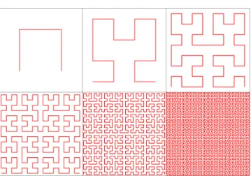
The Hilbert curve H is a continuous fractal space-filling curve, H : [0,1]→[0,1]d, with H([0,1]) = [0,1]d. This curve is not a bijection, because the equation H(x) = y may have more than one solution in x(for a fixedy); the set of such pointsy is of Lebesgue measure 0. In our framework, the interesting point is that the functionH admits however a pseudo-inverseh: [0,1]d→[0,1], i.e. a functionhsuch thatH(h(y)) =y for all
x∈[0,1]d. The functionH is obtained as a limit of the iterative process depicted by Figure 1. We refer to the book of [Sag94] for more details on the properties of space-filling curves.
Figure 1. First steps of the iterative process, the limit of which is the Hilbert curve in two dimensions (Source: Wikipedia).
In the SQMC context, we will usehto transform theNancestors into points in [0,1], before using the inverse CDF as fordx= 1. More precisely, instead of constructing a Monte Carlo approximation of
N X n=1 Wtn−1nδxn t−1(dxt−1)×f X(dxt|xt −1) o
we construct a low-discrepancy approximation of N X n=1 Wtn−1nδh◦ψ(xn t−1)(dh)×f X(dxt|xt −1) o
whereψ is some user chosen transformation, fromRdx to [0,1]d, so that indeed h◦ψ(xn
t−1)∈[0,1]. Thus, one
may proceed as follows: first, find permutation σsuch that h◦ψ(xσt−(1)1)≤. . .≤h◦ψ(xσt−(n1)); then, exactly as before, and for eachn, findmsuch that
m−1 X p=1 Wtσ−(1p)≤unt ≤ m X p=1
Wtσ−(p1) (empty sum equals 0)
and set an
t =n. The rest of the Algorithm is unchanged; see Algorithm 4.
Although we have motivated the Hilbert curve in this short description as a practical way to “project” the
N ancestors into [0,1], there are more fundamental reasons why the Hilbert curve is a particularly convenient transformation in the context of SQMC. In a few words, the Hilbert curve (and its inverse) preserves discrepancy in some sense, that is, if the ancestors xnt−1 have low discrepancy, then so will have the h(xnt−1). This point turns out to be essential when establishing the convergence properties of SQMC, (see [GC14] for a sharper description of this important point).
2.1.6. Concluding remarks
The main advantage of SQMC approach over standard particle filtering is the faster convergence, asN → ∞. We refer to [GC14] for a formal convergence results that support this statement, and several simulation studies, where improvement factors range from 10 to 105 (in the sense that SMC would need 10 to 105 more particles
Algorithm 4SQMC algorithm At timet= 0,
(a): Generate a QMC point setu1:0N in [0,1]d, and computexn0 = Γ0(un0) for eachn= 1, . . . , N.
(b): Computewn0 =G0(x0n) andW0n=wn0/
PN
m=1w
m
0 for eachn= 1, . . . , N.
Iteratively, from timet= 1 to timet=T,
(a): Generate a QMC point setu1:tN in [0,1]d+1; letunt = (unt,vtn)∈[0,1]×[0,1]d. (b): Hilbert sort: find permutationσt−1such thath◦ψ(x
σt−1(1) t−1 )≤. . .≤h◦ψ(x σt−1(N) t−1 ) ifd≥2, or xσt−1(1) t−1 ≤. . .≤x σt−1(N) t−1 ifd= 1.
(c): Find permutation τ such thatuτt(1)≤...≤uτt(N), generatea1:N
t−1 using Algorithm 3, with inputs
uτt(1:N)andWσt−1(1:N) t−1 , and computexnt = Γt(x σt−1(ant−1) t−1 ,v τ(n) t ) for eachn= 1, . . . , N. (e): Computewn t =Gt(x σt−1(ant−1) t−1 ,xnt), andWtn =wnt/ PN m=1w m t for eachn= 1, . . . , N.
More generally, QMC is now widespread in Bayesian statistics and seems to have been slightly overlooked in Bayesian computation, at least up to now. We expect that the advent of SQMC will hopefully change this state of affair.
2.2.
A nonparametric analysis of Approximate Bayesian Computation (ABC)
Let us recall that`(Y|θ) refers to the distribution (likelihood) of the random variableY, whereθ∈Θis an unknown parameter that we wish to estimate, with a prior distributionπ. In the sequel, we still denoteπ(θ) the density ofπwith respect to the Lebesgue measure onRpand the observation vector is denotedy
n= (Y1, . . . , Yn). Before we go into more details onabc, some more notations are required. We assume to be given a statistic S, taking values inRm. It is a function of the random variable Y, with a dimensionmtypically much smaller
than the dimension of Y. The statisticS is supposed to admit a conditional density f(s|θ) with respect to the Lebesgue measure on Rm. Strictly speaking, we should write S(Y) instead of S. However, since there
is no ambiguity, we continue to use the latter notation. As such, the statistic S should be understood as a low-dimensional summary of yn. For example, it can be a sufficient statistic for the parameter Θ, but not necessarily. Assuming that the prior distribution on Θ is absolutely continuous with respect to the Lebesgue measure on Rp, the conditional distribution on Θ given S=s has a density g(θ|s). According to the Bayes
rule, this conditional density takes the form
g(θ|s) = f(s|¯θ)π(θ)
f(s) , where ¯f(s) =
Z
Rp
f(s|θ)π(θ)dθ
is the marginal density of S. Finally, we denote bys0 the observed realization ofScomputed on the data set
yn. Throughout the document, s0 and yn should be considered as fixed quantities (n refers to the number of observed data generated) although N will be the number of simulations (or particles) simulated by the abc. As stressed in [MPRR12], a classical formulation ofabcis the following one:
Algorithm 5Pseudo-code of a genericabcalgorithm
Require: A positive integerN, an integerkN between 1 andN, an observation vector ynands0.
Require: A sampling algorithm ofπand a sampling algorithm of observationsY ∼`(.|θ). fori= 1 toN do
Generateθi in Θ from the priorπ; Generate annsampleyi= (Yi
1, . . . , Yni) from the tensorized law⊗n`(.|θi). end for
return Theθi’s such that Si=S(yi) is among thek
In practice, the parameterNshould be chosen very large (typically of the order of 106), whilek
N is commonly expressed as a percentile ofN. Thus, for example, the choiceN = 106 and a percentilek
N/N = 0.1% allow to retain 1000 simulatedθi’s.
From a nonparametric perspective, this algorithm falls within the broad family of nearest neighbor-type proce-dures [FH51,LQ65,Cov68]. In order to better understand the rationale behind it, denote by (θ1,y1), . . . ,(θN,yN) an i.i.d. sample, with common joint distribution `n(y|θ)π(θ). This sample is naturally associated with the i.i.d. sequence (θ1,S1), . . . ,(θN,SN), where each pair has a densityf(s|θ)π(θ). Finally, letS(1), . . . ,S(kN) be thekN-nearest neighbors ofSn amongS1, . . . ,SN, and letθ(1), . . . ,θ(kN)be the correspondingθi’s. With this
notation, we see that the genericabcAlgorithm 5 proceeds in two steps: (1) First, simulate (realizations of) anN-sample (θ1,yn1), . . . ,(θN,ynn); (2) Seconds, return (realizations of) the variablesΘ(1), . . . ,Θ(kN).
As will become clear in Section 2.2.1, this simple observation opens the way to a mathematical analysis ofabc via statistical methods based on the nearest neighbors. For now, let us just specify that for a fixed s0 ∈Rm,
the estimate we will consider to infer the posterior densityg(.|s0) at some pointθ0∈Rpis
ˆ gN(θ0) = 1 kNhpN kN X j=1 K θ 0−θ(j) hN , (7)
where {hN}N≥0 is a sequence of positive real numbers (bandwidth) andK is a nonnegative Borel measurable
function (kernel) onRp. To reduce the notational burden, we dropped the dependency of the estimate upons0,
keeping in mind that s0 is held fixed. The idea is simple: in order to estimate the posterior, just look at the
kN-nearest neighbors ofs0and smooth the correspondingθj’s aroundθ0. It should be noted that (7) is a smart
hybrid between ak-nearest neighbor and a kernel density estimation procedure. In particular, it is different from the Rosenblatt-type [Ros69] kernel conditional density estimates proposed in [BZB02] and analyzed in [Blu10]. To conclude this introduction, we would like to make a few comments on the topics that willnotbe addressed in the following. An important part of the performance of theabc approach, especially for high-dimensional data sets, relies upon a good choice of the summary statistic S. In many practical applications, this statistic is picked by an expert in the field, without any particular guarantee of success. A systematic approach to choosing such a statistic, based upon a sound theoretical framework, is currently under active investigation in the Bayesian community. This important issue will not be pursued further here. As a good starting point, the interested reader is referred to [JM08], who develop a sequential scheme for scoring statistics according to whether their inclusion in the analysis will substantially improve the quality of inference. Similarly, we will not address issues regarding how to enhance efficiency of abcand its variants, as for example with the sequential techniques of [SFT07] and [BCMR09]. Nor won’t we explore the important question ofabcmodel choice, for which theoretical arguments are still missing [RCMP11, MPRR11]. Finally, we refer the reader to [BCG12] for details and proofs concerning the upcoming results.
2.2.1. Distribution ofabcoutputs
We recall that (θ1,S1), . . . ,(θN,SN) are i.i.d. Rp×Rm-valued random variables, with common probability
density f(θ,s) = f(s|θ)π(θ). Both Rp and Rm are endowed with the Euclidean norm k.k. In this section,
attention is focused on the distribution of the algorithm outputs (θ(1),S(1)), . . . ,(θ(kN),S (kN)).
In what follows, we denote by di the (random) distance between s0 and Si. Similarly, we let d(i) be the
distance betweens0and itsi-th nearest neighbor amongS1, . . . ,SN, that isd(i)=kS(i)−s0k.It turns out that,
conditionally on d(kN+1), one can consider thekN-tuple (θ(1),S
(1)), . . . ,(θ (kN),S
(kN)) as an ordered sample
drawn according to the probability density
1[ks−s0k≤d(kN+1)]f(θ,s) Z Rp Z Bm(s0,d(kN+1)) f(θ,s)dθds ,
where Bm(s0, δ) stands for the closed ball in Rm centered at s0 with nonnegative radiusδ. Alternatively, the
(unordered) simulated values may be treated like i.i.d. realizations of variables with common density proportional to1[ks−s0k≤d(kN+1)]f(θ,s). Thus, givend(kN+1), the acceptedθj’s are i.i.d. realizations of the probability density
Z Bm(s0,d(kN+1)) f(θ,s)ds Z Rp Z Bm(s0,d(kN+1)) f(ϑ,s)dϑds .
Although this conclusion is intuitively clear, its proof requires a careful mathematical analysis (see [BCG12]). Moreover, it plays a key role in the mathematical analysis of the conditional density estimate (7) associated with abcmethodology. In fact, investigating abcin terms of nearest neighbors has other important consequences. Suppose, for example, that we are interested in estimating some finite conditional expectation E[ϕ(θ)|S=s0],
where the random variable ϕ(θ) is bounded. If Θ is itself bounded, it includes in particular the important setting where ϕ is polynomial and one wishes to estimate the conditional moments of θ. Then, provided
kN/log logN → ∞ andkN/N →0 as N → ∞, it can be shown thepointwise consistency, which means that for almost alls0(with respect to the distribution ofS), with probability 1,
1 kN kN X j=1 ϕ θ(j) →E[ϕ(θ)|S=s0]. (8)
The proof of such a result uses a sharp statistical analysis of the nearest neighbor estimation ability. To be more precise, let us consider an i.i.d. sample (X1, Z1), . . . ,(XN, ZN) taking values inRm×R, where the output
variables Zi’s are bounded. Assume that theXi’s have a density and that our goal is to assess the regression functionr(x) =E[Z|X=x],x∈Rm. Then thek-nearest neighbor regression function estimate ofrtakes the
form ˆ rN(x) = 1 kN kN X j=1 Z(j), x∈Rm,
whereZ(j)is theZ-observation corresponding toX(j), thej-th-closest point toxamongX1, . . . ,XN. Denoting
by µ the distribution of X1, it is proved in Theorem 3 of [Dev82] that provided kN/log logN → ∞ and
kN/N → 0, then forµ-almost all x, ˆrN(x) goes to r(x) with probability 1 asN goes to ∞. This result can be transposed without further effort to ourabcsetting via the correspondenceϕ(θ)↔Z andS↔X, thereby stating (8).
2.2.2. Mean square error consistency
Our next objective is to estimate the posterior density g(θ0|s0), θ0 ∈ Rp. This estimation step is an
important ingredient of the Bayesian analysis, whether this may be for visualization purposes or more involved mathematical achievements. As exposed in the introduction, a natural abc-companion estimate of g(θ0|s0)
takes the form (7). Our goal in this section is to investigate some consistency properties of this estimate. Pointwise mean square error consistency is proved in Theorem 2.1 and mean integrated square error consistency is established in Theorem 2.2. We stress that this part of the document is concerned with minimal conditions of convergence. However, the following assumptions on the kernel will be needed:
Assumption [K1] The kernelK is nonnegative and belongs toL1(
Rp), withRRpK(θ)dθ= 1. Moreover, the
functionθ∈Rp7−→sup
kyk≥kθk|K(y)|is inL1(Rp).
Assumption set [K1] is in no way restrictive and is satisfied by all standard kernels such as, for example, the uniform kernel or the Gaussian kernel. In the following, we denote by λp (respectively, λm) the Lebesgue
measure onRp (respectively,
Rm) and set, for any positiveh, Kh(θ) = 1 hpK θ h , θ∈Rp.
We note once and for all that Assumption [K1] implies that R
RpKh(θ)dθ = 1. We are now in a position to
state the two main results of this section.
Theorem 2.1 (Pointwise mean square error consistency). Assume that the kernelK is bounded and satisfies Assumption[K1]. Assume, in addition, that the joint probability densityf is such that
Z
Rp
Z
Rm
f(θ,s) log+f(θ,s)dθds<∞. (9)
Then, for λp⊗λm-almost all (θ0,s0) ∈ Rp×Rm, with f¯(s0) > 0, if kN → ∞, kN/N → 0, hN → 0 and
kNh p N → ∞, E[ˆgN(θ0)−g(θ0|s0)] 2 →0 asN → ∞.
It is easy to see that assumption (9) is mild. It is for example satisfied wheneverf is bounded or whenever
f belongs to Lq(
Rp×Rm) with q >1. Theorem 2.2 below says that ˆgN is also consistent with respect to the mean integrated square error criterion. Here again, the regularity assumptions onf andπare minimal. Theorem 2.2 (Mean integrated square error consistency). Assume that the kernel K belongs to L2(
Rp)and
satisfies Assumption [K1]. Assume, in addition, that the joint probability density f and the prior π are in
L2(Rp×Rm) and L2(Rp), respectively. Then, for λm-almost all s0 ∈ Rm, with f¯(s0) > 0, if kN → ∞,
kN/N →0,hN →0 andkNhpN → ∞, E Z Rp [ˆgN(θ0)−g(θ0|s0)] 2 dθ0 →0 asN → ∞. 2.2.3. Rates of convergence
In this section, we go one step further in the analysis of the abc-companion estimate ˆgN by studying its mean integrated square error rates of convergence. As before, we keep trying to alleviate the assumptions on the unknown mathematical objects as mild as possible. We introduce the multi-index notation
|β|=β1+. . .+βn, β! =β1!. . . βn!, xβ =xβ11. . . x
βn
n
forβ = (β1, . . . , βn)∈Nnandx∈Rn. If all thek-order derivatives of some functionϕ:Rn→Rare continuous
atx0∈Rn then, by Schwarz’s theorem, one can change the order of mixed derivatives atx0, and the notations
Dβϕ(x0) = ∂|β|ϕ(x 0) ∂xβ1 1 . . . ∂x βn n , |β| ≤k
for the higher-order partial derivatives are thus justified in this situation. Recall that the collection of all s0 ∈Rm withRBm(s0,δ)
¯
f(s)ds>0 for all δ >0 is called the support of ¯f. We shall need the following set of assumptions.
Assumption [A1] f¯has a compact support included in a ball of diameterL >0 and is three times continu-ously differentiable.
Assumption [A2] The joint probability densityf is inL2(
Rp×Rm). Moreover, for fixed s0, the functions
θ07→ ∂2f(θ0,s0) ∂θi1∂θi2 , 1≤i1, i2≤p and θ07→ ∂2f(θ0,s0) ∂s2 j , 1≤j≤m,
are defined and belong toL2(
Rp).
Assumption [A3] f is three times continuously differentiable on Rp×
Rmand, for anyβ satisfying|β|= 3,
sup s∈Rm Z Rp Dβf(θ,s)2 dθ<∞. Assumption [K2] Kis symmetric, is inL2(
Rp), and for anyβsuch that|β| ∈ {1,2,3},RRp
θ
β
K(θ)dθ<∞.
Recall that s0 is called a Lebesgue point if
1 λm(Bm(s0, δ)) Z Bm(s0,δ) f¯(s)−f¯(s0) ds→0 as δ→0.
Lebesgue’s differentiation theorem asserts that this is true forλm-almost alls0∈Rm. Ifs0 is a Lebesgue point
of ¯f such that ¯f(s0)>0, then it is readily seen that
0< ξ0= inf 0<δ≤L 1 δm Z Bm(s0,δ) ¯ f(s)ds<∞.
Let us mention that Lebesgue points are commonly encountered when dealing with Nearest Neighbor rule. This was already pointed in the seminal work of [Dev82], and thereafter extended by considering “Besicovitch” conditions in [CG06]. Some recent developments in [GKM14] have even established that this kind of “mini-mal mass assumption” on s“mini-mall balls are unavoidable in general finite dimensional spaces to derive uniform consistency rates of classification (with any classifier).
Theorem 2.3 (Rates of convergence). Suppose that assumptions [K1]-[K2] and[A1]-[A3] are satisfied. Let
s0 be a Lebesgue point off¯such thatf¯(s0)>0. Denote
φ1(θ0,s0) = 1 2 p X i1,i2=1 ∂2f(θ 0,s0) ∂θi1∂θi2 Z Rp θi1θi2K(θ)dθ and Φ1(s0) = 1 ¯ f2(s 0) Z Rp φ21(θ0,s0)dθ0, φ2(θ0,s0) = 1 2m+ 4 m X j=1 ∂2f(θ 0,s0) ∂s2 j and Φ2(s0) = 1 ¯ f4(s 0) Z Rp φ2(θ0,s0) ¯f(s0)−φ3(s0)f(θ0,s0) 2 dθ0 φ3(s0) = 1 2m+ 4 m X j=1 ∂2f¯(s0) ∂s2 j and Φ3(s0) = 2 ¯ f3(s 0) Z Rp φ1(θ0,s0)φ2(θ0,s0) ¯f(s0)−φ3(s0)f(θ0,s0)dθ0.
Then, for m >4, there exist sequences {kN} with kN ∝N
p+4 m+p+4 and{hN} withhN ∝N− 1 m+p+4 such that E Z Rp [ˆgN(θ0)−g(θ0|s0)] 2 dθ0 = mΦ1(s0) ξ04/m(m−4) + Φ2(s0) + mΦ3(s0) ξ02/m(m−2) + Z Rp K2(θ)dθ+ o(1) ! N−m+4p+4.
Three concluding remarks are in order:
(1) From a practical perspective, the fundamental problem is that of the joint choice ofkN and hN in the absence of a prioriinformation regarding the posterior g(.|s0). Various bandwidth selection rules for
conditional density estimates have been proposed in the literature [BH01, HRL04, FY04]. But most (if not all) of these procedures pertain to kernel-type estimates and are difficult to adapt to our nearest-neighbor setting. Moreover, they are tailored to global statistical performance criteria, whereas the problem here is local sinces0is fixed. Hence, devising a good methodology to automatically select both
(2) Nevertheless, Theorem 2.3 provides an insight into the proportion of simulated values which should be accepted by the algorithm. For example, a rough rule of thumb is obtained by taking kN ≈
N(p+4)/(m+p+4), so that a fraction of aboutk
N/N ≈N−m/(m+p+4)simulations should not be rejected. (3) At last, it should be noted that the size of the statistic S (the integer m) can dramatically damage the convergence rate obtained in Theorem 2.3. It is thus a basic fact to choose a sufficient statistic embedded in the lowest dimensional space possible.
3.
Consistency for an example of nonparametric hidden Markov model
3.1.
The studied model: hidden Markov models with finite state space
We now turn back to a specific case of HMMs introduced in Section 2.1, when then hidden component (xt)t∈Nlives in a finite state space. We are interested in Bayesian consistency results when the observation time
(denotednin what follows) is increasing. We would like to emphasize that such a result should be obtained in a different context as those stated in Section 1.3.1: observations (yt)1≤t≤n are no longer independent here and a significant amount of work is needed to reach Bayesian consistency.
Frequentist asymptotic properties of estimators of HMMs parameters have been studied since the 1990s. Consistency and asymptotic normality of the maximum likelihood estimator have been established in the para-metric case, see [DM01], [DMR04] and [DMOvH11] for the most general consistency results up to now. As to parametric Bayesian asymptotic results, there are only a few recent results, see [dGS08] when the number of hidden states is known and [GR14a] when the number of hidden states is unknown. Because parametric modeling of emission distributions may lead to poor results in practice, in particular for clustering purposes, recent interest in using non parametric HMMs appeared in applications, see [YPRH11], [GCR14] and references therein. Theoretical results for estimation procedures in non parametric HMMs have been obtained only very recently such as in [DLC12] and in [GR13] since even identifiability remained an open problem (see [GCR14]). The studied model is specified here and can be visualized in Figure 2. We still denote the HMMs (xt,yt)t∈N
where x is a homogeneous Markov chain whose transition kernel was previously denoted fX(xt|xt
−1). This
kernel is now simply described as a squared matrix Qsince we assume in this paragraph the finiteness of the state spaceX wherexis living. In the meantime, the conditional probability distribution ofytwhenxtis given was previously denotedfY(yt|xt) and is now shortened asfxt(yt).
µ
X X X X
Y
Y Y Y
fX fX fX fX
Figure 2. Schematic evolution of the HMM with a transition kernel Q and a conditional distributionfx whenx1∼µ.
In what follows, we will assume thatQis strongly irreducible, meaning that there existsq >0 such that ∀(i, j)∈J1, kK Qi,j ≥q.
The former assumption on the transition kernelQimplies that the Markov chainxpossesses a unique invariant distributionµwith an exponential mixing rate. In the meantime, we also assume the chain is initialized with its invariant distribution: x1∼µ.
3.2.
Prior structure
In what follows, we assume that the number k of hidden states, as well asq, is known, so that the state space of the Markov chain is set to {1, . . . , k}. In order to define the set where the prior and the posterior distributions are living, we naturally introduce thek−1-dimensional simplex denoted
∆k(q) ={(p1, . . . , pk) : pi≥q, i= 1, . . . k ; k
X
i=1
pi= 1}.
The transition matrix Qmay be identified as a k-uple of transition distributions (the lines of the matrix), so that Q ∈ ∆k(q)k. We denote µ ∈ ∆k(q) the invariant probability measure, that also initializes the Markov chain at time 1: x1∼µ. We assume that the observation space isRd endowed with its Borel sigma field. Let
F be the set of probability density functions with respect to a reference measure λ on Rd. Fk is the set of
possible emission densities from xt toyt. It means that for any f = (f1, . . . , fk)∈ Fk, the distribution of yt conditionally toxt=iwill befidλfor each value of ibetween 1 andk.
LetΘ={θ= (Q, f) : Q∈∆k(q)k, f∈ Fk}.Remark that a particularθ∈Θimplicitely defines a transition kernelQand therefore a unique invariant distributionµ. For anyθ∈Θ,Pθdenotes the probability distribution of (xt,yt)t∈Nwhen the transitions are parametrized byθ and when the initial statex1 is distributed according
to the invariant distributionµ.
We denote Plθ the marginal distribution of y1, . . . ,yl under Pθ,µ and pθl its corresponding density with respect to λ⊗lunder
Pθ. For anyθ∈Θ associated with an initial probabilityµ, we have: pθl(y1, . . . , yl) =
X
(x1,...,xl)∈J1,kKl
µx1Qx1,x2. . . Qxl−1,xlfx1(y1). . . fxl(yl).
Letπdenotes a prior onΘ, we assume thatπis a product of probability measures onΘ,π=πQ⊗πf such that πQ is a probability distribution on ∆k(q)k andπf is a probability distribution onFk.
3.3.
Posterior consistency
3.3.1. Topological descriptionThe observations are now distributed from Pθ0 where θ
0 = (Q0, f0) so that the distribution of (xt,yt)t≥1
follows a stationary HMM. We are interested in posterior consistency, that is to prove that for all neighborhood
U ofθ0, withPθ0 almost surely:
lim
n→+∞π(U|yn) = 1.
To make the former equality meaningful, it is necessary to define a neighborhood concept ofθ0and a topology
has to be chosen for a precise definition of U. We choose to study posterior consistency for the problem of density estimation,i.e. we want to know if the posterior concentrates its mass around the parameters such that the associated distributionPθ
l oflconsecutive observations is closed to the one associated to the true parameter. We will use two different topologies as in Theorems 1.2 and 1.3. We first use the weak topology on marginal distributions (Pθ
l )θ∈Θ.
Let us briefly recall the definition of a weak neighborhood of Plθ (for the weak topology on probability measures). For any integer N and any set of bounded continuous functions (hj)1≤j≤N from (Rd)l to R, we
denote W pθl, ,(hj)1≤j≤N:= P : Z hjdP − Z hjpθldλ ⊗l < ,∀j∈J1, NK . (10) A weak neighborhood of pθ
l is a set of probability distributionsO such that: ∃N ∈N ∃ >0 ∃(hj)1≤j≤N W pθl, ,(hj)1≤j≤N
We will also work with the finer topology associated to theL1-distance on the joint densities. Other topologies
may be considered depending on the estimation needed, see for example [Ver13] where a product of the topologies for the transition matrix and the emission densities is also used.
3.3.2. Main results
In HMMs,yt may not only depend on the previous observation yt−1 but also on the previous observations
yt−2, . . . ,y1. The generalization of the Hoeffding inequalities [Rio00] requires a level of mixing of the chain to
ensure an exponential rate of concentration (and then the existence of a powerful test between two hypotheses). Since θ0 is such thatQ0 ∈ ∆k(q)k with a known q (non adaptive prior on q), we will only consider priorπQ such that
πQ∆k(q)k = 1 and min
1≤i≤kµi≥q. (11) This ensures a level of mixing of the Markov chains for the possible parameters and that the associated Markov chains are irreducible (and thus positive recurrent sinceX is finite here) and admit a unique stationary proba-bility measure.
Theorem 3.1 describes a set of assumptions that lead to the posterior consistency for the weak topology, and may be compared to Theorem 1.2. The following assumption on the neighborhood of θ0 is used:
Assumption [N] For all >0 small enough, there exists a set Θ ⊂ Θ such that π(Θ) >0 and for all
θ= (Q, f)∈Θ, kQ−Q0k< , (12a) max 1≤i≤k Z fi0(y) max 1≤j≤klog f0 j(y) fj(y) ! λ(dy)< , (12b)
For ally∈Rd such that k X i=1 fi0(y)>0 =⇒ k X j=1 fj(y)>0, (12c) sup y: Pk i=1fi0(y)>0 max 1≤j≤kfj(y)<+∞, (12d) k X i=1 Z fi0(y) log k X j=1 fj(y) λ(dy)<+∞ (12e)
Theorem 3.1. [Ver13] Assume that the priorπ satisfies (11)and that Assumption [N]holds, then for all weak neighborhood U of Pθ0
l (see (10)), lim
n→∞π(U|yn) = 1 P
θ0−a.s.
Theorem 3.1 is proved in [Ver13] using the general method introduced in [Bar88]. Assumption (11) ensures the existence of tests that discriminate the set of hypotheses Pθ whenθ is not in a closed neighborhood ofθ0
for the weak topology. These results are derived by using a generalization of Hoeffding’s inequality by [Rio00] and [GR14a]. Assumption [N] ensures that the prior π gives a positive weight to any Kullback-Leibler neighborhood ofPθ0.
It is also possible to derive a stronger result by using theL1- norm, which defines a finer topology than the
weak one. As in the case of density estimation with i.i.d. observations (Theorem 1.3), an additional assumption on the covering number implies the existence of tests that permit to discriminatePθ to
Pθ0 when dealing with
theL1 distance. For this purpose, we define the distance
∀(f, g)∈ F d(f, g) = max
Assumption [H] For all n >0,for all δ >0 there exists a setFn ⊂ Fk and positive numbersr1, C1 such
that
πf (Fn)c≤C1e−nr1 and such that
X n>0 N δ 36l,Fn, d(·,·) exp −nδ 2k2q2 32l ! <+∞. (13)
Theorem 3.2. [Ver13] Assume that the prior πsatisfies (11)and thatAssumption [N] andAssumption [H] hold, then for allL1-neighborhoodU ofPlθ0, there existsr >0 such that
lim
n→∞π(U|yn) = 1 P
θ0−a.s.
Thanks to the similarities of Assumptions (12b) and (13) with Assumptions (2) and (3) respectively, it may be possible to use consistent priors in the case of density estimation with i.i.d. observations for the emission distribution in HMMs. Such examples are given in [Ver13] for instance in the case of translated emission distributions that is to say when for all 1≤j≤k,
fj(·) =g(· −mj)
where for all 1≤j ≤k,mjis inRandg is a density function onRdistributed from a mixture of Gaussians by
Dirichlet process.
4.
The PAC-Bayesian paradigm
4.1.
Generality on PAC-Bayesian approaches
To illustrate the concepts behind the PAC-Bayesian approach, let us consider the standard regression model y = fθ0(x) +W, where y is a real-valued response, fθ0 : Rd → R is the unknown regression function
de-pending on some parameter θ ∈ Θ, x is ad-dimensional random variable and W is a real-valued noise term. Let us assume that we collect an n-sized sample of i.i.d. replications of the random variable (x,y) denoted (X1, Y1), . . . ,(Xn, Yn). For some loss function`:R×R→(0,∞), we define the risk (and its empirical
counter-part) of some estimatorfˆθoffθ0 as
R(fˆθ) =E[`(y, fˆθ(x))], Rn(fθˆ) = 1 n n X i=1 `(Yi, fθˆ(Xi)). (14) LetR?=R(f
θ0),R? is of course the lowest (oracle) risk that can be reached by any predictorfθ. We aim to
obtain some statistical guarantees involving inequalities in deviations of the excess risk of Bayesian estimators
fθˆ built with a suitable choice of the prior. The nice oracle inequalities we are looking for are generally stated
as follows: ∀ε∈(0,1) P R(fθˆ)−R ?≤K inf θ n R(fθ)−R?+ ∆n,d,M,ε(θ) o ≥1−ε, (15) whereK≥1 is a constant and ∆n,d,M,εis a remainder term which decays asngrows. The message of this work is that when the ambient dimensiondis large with respect to the sample sizen, it is possible with a properly-chosen prior to reach convergence rates ∆n,d,M,εthat are not too badly affected by the curse of dimensionality. Another saliant fact is that this procedure relies on very little assumption on the distribution of the variable (x,y).
We propose to investigate a semi-parametric form for the regression function, allowing for flexibility. We are interested in the situation where the unknowfθ can be sparsely decomposed in an additive model
fθ0(x1, . . . , xd) =
d
X
j=1
and we assume that only a few of (ψ0
j)1≤j≤d influences the response y. This naturally drives us to consider an additive model of the form
fθ(x1, . . . ,xd) = d X j=1 mj X k=1 θjkφk(xj), θ∈Θ=R Pd j=1mj, kfθk ∞≤C ,
where m = (m1, . . . , md) ∈ {0, . . . , M}d is a model, D = {φ1, φ2, . . . , φM} is a known dictionary composed of deterministic functions (or preliminary estimators). Furthermore, C is a known constant that controls the volume of the parameters space in order to be consistent with the learning sample. This additive formulation (see for example [Sto85, HT86]) achieves a nice compromise between flexibility and interpretation.
The PAC approach produces a priori risk bounds (see [Val84]); the additional Bayesian flavor allows us to obtain a posteriori bounds. In what follows, we are especially interested in the situation of a sparse oraclefθ0
to recover. As usual, we considerMthe set of measures onΘ that are absolutely continuous with respect to a reference measuredθ. We naturally wish to use a prior probability measureπ∈ M promoting sparsity. For this purpose, we consider the following constrained optimization problem:
arg min ρ∈M Z Θ Rn(fθ)ρ(dθ) + λ nKL(ρ, π) , (16)
where the Kullback-Leibler divergence is defined as ∀ρ∈ M KL(ρ, π) = Z Θ log dρ dπ(θ) ρ(dθ).
Indeed, the (frequentist) variational formulation of (16) may be interpreted as a Bayesian formulation (justifying the interpretation ofπas a prior distribution). In fact, it is an exercise to check that (16) has a unique solution, which is the so-calledGibbs posterior distribution
ˆ
ρλ(dθ)∝exp[−λRn(fθ)]π(dθ).
Hence, the penalization parameter λ > 0 may be seen as an inverse temperature parameter of the Gibbs distribution. From the Gibbs posterior distribution ˆρλ, two estimators are considered in this document:
ˆ
θ∼ρˆλ (Randomized estimator sampled with the posterior), ¯
θ=
Z
Θ
θρˆλ(dθ) =Eρˆλθ (Posterior mean).
As shown it will be shown below, PAC-Bayesian theory is a great tool to produce estimators with nearly minimax optimal properties. The first important result for PAC-Bayesian theory is the standard link between the Legendre transform of the Kullback-Leibler divergence and a Gibbs fields.
Lemma 4.1 ( [Csi75]). Let (A,A) be a measurable space. For any probability measure µ on (A,A) and any measurable functionh:A→Rsuch thatR(exp◦h)dµ <∞,
log Z (exp◦h)dµ= sup m∈M1 µ(A,A) Z hdm− KL(m, µ) ,
with the convention ∞ − ∞= −∞. Further, if h is upper-bounded on the support of µ, the supremum with respect to min the right-hand term is reached for the Gibbs distributiong defined by
dg
dµ(a) =
exp◦h(a)
R
The second important result is the following concentration inequality (seee.g.[Mas07]).
Lemma 4.2 (Bernstein’s inequality). Let(Ti)ni=1be a collection of real independent random variables. Assume
there exist two positive constants v andwsuch that
n
X
i=1
ETi2≤v,
and for any integerk≥3,
n X i=1 E[(Ti)k+]≤ k! 2vw k−2.
Then, for anyγ∈ 0, 1
w , E " exp γ n X i=1 (Ti−ETi) !# ≤exp vγ2 2(1−wγ) .
PAC-Bayesian bounds depend on the Kullback-Leibler divergence and hold for any priorπ. In order to obtain an optimized PAC-Bayesian estimator, two levers are at our disposal: the inverse temperature parameterλand the priorπ. These two key quantities must be well-tailored to obtain some good oracle inequalities. In particular, we may consider a sparsity-inducing prior, such as
πs(θ)∝X m d |m|0 −1 βPdj=1mj Unif Bm(C)(θ),
whereβ ∈(0,1) andBm(C) is the`1 sphere of radiusC:
Bm(C) = θ, d X j=1 mj X k=1 |θjk| ≤C .
This prior distributionπsdefined above satisfies the nice property to favor sparse parameters (it gives a highest mass to the parameters with a low`0 norm of the coefficients (mj)
1≤j≤d).
4.2.
Examples
The work [GA13] provides several practical examples detailed below. 4.2.1. Regression models
We consider the standard model
y=ψ?(x) +w,
with two mild assumptions.
Assumption 1: The noise is subexponential: • For any integerk≥2,E[|w|k]<∞. • E[w|x] = 0.
• There exist two positive constantsL,σ2 such that, for any integerk≥2,
E[|w|k|x]≤ k!
2σ
2Lk−2.
Assumption 2: |ψ?| ∞≤C.
In particular, Assumption 1 is met if w has a Gaussian distribution. As for Assumption 2, it allows to use concentration inequalities such as Lemma 4.2. From what precedes, we obtain the following oracle inequality.
Theorem 4.3 ( [GA13]). For anyε∈(0,1), any0< λ < n/(4σ2+ 4C2), with probability at least1−ε, R(fθˆ)−R(ψ?) R(fθ¯)−R(ψ?) ≤Kλ×inf m θ∈Bminf(C) R(fθ)−R(ψ?) +|m|0 log(d/|m|0) n + log(n) n d X j=1 mj+ log(2/ε) n , where Kλ−−−→ λ→0 1 and Kλ−−−−−−−−−−→λ→n/(4σ2+C2) +∞.
4.2.2. Case of Sobolev space
In certain function space, it is possible to derive some minimax optimality properties. Assume that ψ∗ is indeed an additive form of nonparametric decomposition in a Sovolev space, for example say ψ? =P
j∈S?ψj?, and letφ1, φ2, . . . refer to the trigonometric basis. Assume that each of theψj∗s belong to a Sobolev ellipsoid:
ψj?∈ W(rj, `j) = ( f ∈L2([−1,1]) :f = ∞ X k=1 θkφk and ∞ X i=1 i2rjθ2 i ≤`j ) ,
where rj’s are unknown regularity parameters, casting our results onto the adaptive setting. We obtain the following oracle inequality.
Theorem 4.4 ( [GA13]). For any realε∈(0,1), any 0< λ < n/(4σ2+ 4C2), with probability at least 1−ε,
R(fˆθ)−R(ψ?) R(f¯θ)−R(ψ?) ≤Kλ× X j∈S? ` 1 2rj+1 j log(n) 2nrj 2rj 2rj+1 +|S ?|log(d/|S?|) n + log(2/ε) n .
The message carried by these inequalities is that if there exists a sparse representation of the regression function, then the right-hand side terms become negligible and the excess risk of the PAC-Bayesian estimators mimics the best excess risk one could achieve in the collection. Moreover, the excess loss appears to be minimax up to a log term.
4.2.3. Logistic Regression
This PAC-Bayesian approach has been extended by [Gue13a] to the logistic regression model: y = {±1}, model
log P(y= 1|x)
1−P(Y = 1|x) =ν(x), x∈R
d. The logistic loss function is thus defined as
`: (y, fθ(x))7→log [1 + exp(−yfθ(x))].
Then the link function ν is estimated by the same collection of additive combinations of elements of the dictionary, as before. Similar oracle inequalities are provided in [Gue13a].
4.2.4. Binary Ranking
Note that the PAC-Bayesian tools can also be usedto solve the binary ranking problem in a high-dimensional setting (seee.g.[GR14b]).
The bipartite ranking problem consists in learning from a sample Dn = {(xi,yi)}n
i=1 to rank observations
xi, while preserving the order of their associated labels yi ∈ {±1}. We consider this problem in the high dimensional situation, where the observations (xi)1≤i≤nlie in a space of dimensiond, possibly much larger than the sample size n. A standard approach in this context involves the introduction of a scoring function. We propose to estimate the optimal scoring function using the so-called Gibbs posterior distribution, which favors sparse additive estimators. This procedure appears valuable to assess the effect of each covariate on the score