Statistical and simulation-based modelling approaches for causal inference in longitudinal data: Integrating counterfactual thinking into established methods for longitudinal data analysis

(1)

Statistical and simulation-based modelling approaches for causal

inference in longitudinal data

Integrating counterfactual thinking into established methods for longitudinal data analysis

Kellyn Fair Arnold

Submitted in accordance with the requirements for the degree of Doctor of Philosophy

The University of Leeds School of Medicine

(2)

(3)

The candidate confirms that the work submitted is her own, except where work which has formed part of jointly-authored publications has been included. The contribution of the candidate and the other authors to this work has been explicitly indicated below. The candidate confirms that appropriate credit has been given within the thesis where reference has been made to the work of others.

Chapter 3 contains work based on the following publications:

1. Arnold, K.F., Berrie, L., Tennant, P.W.G. and Gilthorpe, M.S. A causal inference perspective on the analysis of compositional data. International Journal of Epidemiology. 2020, 0(0), pp.1-7. (1)

Kellyn F. Arnold drafted the manuscript and produced all figures together with Dr Lauren Berrie. All authors conceived the idea and revised the manuscript.

2. Arnold, K.F., Davies, V., de Kamps, M., Tennant, P.W.G., Mbotwa, J. and Gilthorpe, M.S. Reflections on modern methods: Generalised linear models for prognosis and intervention – theory, practice, and implications for machine learning. International Journal of Epidemiology. 2020, 0(0), pp.1-9. (2)

Kellyn F. Arnold researched the literature, performed all analyses, produced all figures, and drafted the manuscript. Prof Mark S. Gilthorpe conceived the manuscript and, along with all co-authors, developed the ideas contained in the manuscript and revised the manuscript.

3. Arnold, K.F., Harrison, W.J., Heppenstall, A.J. and Gilthorpe, M.S. DAG-informed regression modelling, agent-based modelling and microsimulation modelling: a critical comparison of methods for causal inference. International Journal of Epidemiology. 2019, 48(1), pp.243-253. (3)

Kellyn F. Arnold researched the literature, performed all analyses, produced all tables and figures, and drafted the manuscript. All other co-authors revised the manuscript. Chapter 4 contains work based on the following publication:

4. Tennant, P.W.G., Arnold, K.F., Ellison, G.T.H. and Gilthorpe, M.S. Analyses of ‘change scores’ do not estimate causal effects in observational data. ArXiv e-prints. [Online]. 2019. (4)

Kellyn F. Arnold researched the literature with Dr Peter W. G. Tennant, performed all path tracing analyses, and rewrote the manuscript into its current form. Prof Mark S. Gilthorpe conceived the study and, along with Dr Peter W. G. Tennant and Kellyn F. Arnold, developed the ideas contained in the manuscript. Dr Peter W. G. Tennant and Prof Mark S Gilthorpe conceived and wrote the simulations, and all authors were involved in their analysis. Prof Mark S. Gilthorpe and Dr George T. H. Ellison revised the manuscript.

(4)

Chapter 5 contains work based on the following publication:

5. Arnold, K.F., Ellison, G.T.H., Gadd, S.C., Textor, J., Tennant, P.W.G., Heppenstall, A. and Gilthorpe, M.S. Adjustment for time-invariant and time-varying confounders in

‘unexplained residuals’ models for longitudinal data within a causal framework and associated challenges. Statistical Methods in Medical Research. 2019, 28(5), pp.1347-1364. (5)

Kellyn F. Arnold researched the literature, performed all analyses and simulations, wrote all mathematical proofs, produced all tables and figures, and drafted the manuscript. Prof Mark S. Gilthorpe conceived the study and, along with all other co-authors, revised the manuscript.

This copy has been supplied on the understanding that it is copyright material and that no quotation from the thesis may be published without proper acknowledgement.

The right of Kellyn Fair Arnold to be identified as Author of this work has been asserted by her in accordance with the Copyright, Designs and Patents Act 1988.

(5)

Acknowledgments

Research is not conducted in a cultural or political vacuum. The years I have spent doing my PhD have been some of the most unsettled and unsettling I have known. The last four years have seen Donald Trump be elected president of the United States; a vote for Brexit and ultimately a withdrawal from the European Union; a rise in nationalism, racism, xenophobia, and polarisation throughout the world; and a global pandemic that rages on – refusing to respect international borders or academic deadlines. It is in this context that I feel particularly obliged to acknowledge and thank the people who have helped make the last four years productive, meaningful, and enjoyable.

First and foremost, I must thank my supervisors Mark Gilthorpe, Alison Heppenstall, and Wendy Harrison, for your constant support, guidance, and encouragement. To Mark, in particular, thank you for recognising my potential and for bringing me into your group of eccentric and eclectic researchers. I have always felt my ideas and skills to be valued, and could not have asked for a better PhD experience. To Alison, thank you for being a voice of reason, pragmatism, and optimism; I am constantly in awe of the way you balance so many things at once.

I am also immensely grateful to my colleagues Laurie Berrie, Peter Tennant, and George Ellison, who have provided endless amounts of creativity and support throughout my years as a PhD student. My research would not be half as good if I were not in such a stimulating and collaborative environment, nor would I enjoy it half as much. To George, thank you for always providing a new and unique perspective. To Peter, thank you for being a constant engine of creativity, and for always being available to give support and advice. To Laurie, thank you for leading the way and being an exemplar of how to get through the challenges of a PhD with poise and grace.

This research would not have been possible without the financial support of the Economic and Social Research Council, who provided me with a generous stipend that has allowed me to live comfortably and travel frequently.

Thank you to the Leeds branch of Women in Biostatistics – Mary Cronin and Sulia Celebi. You are two of the most authentic, intelligent, and unique women I know, and I am proud to call you my friends. I could not have made it through this process without your steadfast emotional support, deliciously imaginative pasta recipes, endless banter, and crazy nights in Ibiza. Thank you also to Andrea Bovo for never allowing me to take myself too seriously, and for having the courage to approach a stranger in a corridor. You have all become my family in Leeds and I love you dearly.

Thank you to my Leeds Medics and Dentists Football Club teammates for keeping me young (if not always in one piece).

(6)

Thank you also to my viva voce examiners – Theresa Munyombwe and Anna Pearce – for a stimulating and enjoyable examination experience.

Possibly my greatest thanks must go to my family, without whom I could not have even arrived at the point where completing a PhD was possible. Thank you for always encouraging me to follow my own path, for being the lender of last resort, and for supporting me from afar throughout this entire process. Despite the many holidays I have missed and birthdays I have forgotten, you have always been by my side.

Finally, I would like to acknowledge and thank all the badass women who carry on doing science in an increasingly hostile world. I am proud to be one of you.

(7)

Abstract

The counterfactual framework represents the dominant paradigm for testing and evaluating causal claims within epidemiology. What began as a philosophical framework has been formalised mathematically in the language of directed acyclic graphs (DAGs), whose

underpinning theory provides a rigorous mathematical framework for the identification and estimation of causal effects. Moreover, DAGs provide a conceptual framework for thinking though causal processes and explicating causal assumptions.

Advances in DAG-based methods are invaluable in the era of ‘big data’, since we are

increasingly awash with large, complex – and frequently longitudinal – datasets. However, the relative recentness of such developments means that many established methods for analysing observational data have not been considered within a robust causal framework.

This PhD thesis explores how counterfactual thinking, encoded in the language of DAGs, may be integrated into established methods for longitudinal data analysis, and illustrates several advantages of doing so. Three statistical- and simulation-based methods are considered: (1) the analysis of change, (2) regression with ‘unexplained residuals’, and (3) microsimulation modelling. For each method, DAGs are specifically employed to consider causal structures and to explore potential problems and/or biases that might arise when these methods are applied without sufficient consideration for such structures. In (1), DAGs are used to demonstrate that ‘change scores’ do not in general represent exogenous change; alternate analytical strategies for isolating change are identified. In (2), DAGs are employed to illustrate why the method works and how it may be extended to adjust for confounding. In (3), DAGs are used to explicitly consider data-generating processes, and to demonstrate some of the unique challenges faced by simulation approaches. DAGs are demonstrated to be useful tools for informing causal analyses across a wide variety of longitudinal scenarios, thereby providing a basis for integrating counterfactual thinking into other methods for longitudinal data analysis.

(8)

(9)

List of tables

Table 3.1 A sample of the stated research objectives for published studies which have examined obesity using DAG-informed regression modelling, microsimulation modelling, and agent-based modelling ... 36 Table 4.1 Total association between 𝑿𝟎 and each of ∆𝒀 and 𝒀𝟏, subdivided into causal

and confounding associations, for the path diagram depicted in Figure 4.2 ... 48 Table 4.2 Total association between 𝑿𝟎 and each of ∆𝒀 and 𝒀𝟏, subdivided into causal

and confounding associations, for the path diagram depicted in Figure 4.3 ... 49 Table 4.3 Total association between 𝑿𝟎 and each of ∆𝒀 and 𝒀𝟏, subdivided into causal

and confounding associations, for the path diagram depicted in Figure 4.4 ... 51 Table 4.4 Median regression coefficient of 𝑾𝑪𝟎 (and 95% simulation limits) for each

method of analysis, for each causal scenario depicted in Figure 4.6 ... 57 Table 5.1 Description of key properties of UR models for a time-varying exposure 𝑿

measured at two time points (i.e. 𝑿𝟎 and 𝑿𝟏) and one outcome 𝒀 ... 67 Table 5.2 Comparing standard regression models and UR models using the method of

path coefficients ... 69 Table 6.1 Table describing the true population average causal effect of each intervention on diabetes prevalence in the simulated population ... 95 Table 6.2 Table describing the estimated causal effect of each intervention on diabetes

prevalence, for each of A1 through A3 modelled using the g-formula, compared to the true effect in the population ... 99 Table 6.3 Table describing the estimated causal effect of each intervention on diabetes

prevalence, for each of the autocorrelation structures modelled using

microsimulation, compared to the true effect in the population ... 104 Table 6.4 Table describing the estimated causal effect of each intervention on diabetes

prevalence for each of AS1 through AS3 modelled using the g-formula and

microsimulation, compared to the true effect in the population (Sensitivity analysis 5) ... 111 Table 7.1 Key messages for epidemiological and public health researchers ... 116 Table A.1 Mean (SD) of waist circumference and insulin concentration, as reported in

three separate waves of NHANES data and as simulated ... 126 Table A.2 Median regression coefficient of 𝑾𝑪𝟎 (and 95% simulation limits) for each

method of analysis, for each causal scenario depicted in Figure A.2 ... 127 Table B.1 Description of key properties of UR models for a longitudinal exposure 𝑿

measured at 𝑻 time points (i.e. 𝑿𝟎, 𝑿𝟏, … , 𝑿𝑻 − 𝟏) and one outcome 𝒀... 132 Table B.2 Correlation matrix implied by the DAG in Figure B.1 ... 143 Table B.3 Population mean and standard deviation (SD) used in the data simulation based

on the DAG in Figure B.1 ... 143 Table C.1 Parameters describing the joint distribution of sex, obesity, and diabetes in the baseline population (i.e. time 𝒕 = 𝟎) ... 148

(16)

Table C.2 Transition parameters describing the evolution of the baseline population (i.e. time 𝒕, for 𝟏 ≤ 𝒕 ≤ 𝟏𝟎) ... 149 Table C.3 Transition parameters governing obesity status at time 𝒕 for Interventions 1

through 6, compared to those of the natural history ... 159 Table C.4 Parameters describing the joint distribution of sex, obesity, and diabetes in the baseline population (i.e. time 𝒕 = 𝟎) for each sensitivity analysis, compared to the original simulation ... 207 Table C.5 Transition parameters describing the evolution of the baseline population (i.e.

time 𝒕, for 𝟏 ≤ 𝒕 ≤ 𝟏𝟎) for each sensitivity analysis, compared to the original simulation ... 208 Table C.6 Table describing the estimated causal effect of each intervention on diabetes

prevalence for each autocorrelation structure modelled using the g-formula and microsimulation, compared to the true effect in the population (Sensitivity analysis 1) ... 210 Table C.7 Table describing the estimated causal effect of each intervention on diabetes

prevalence for each autocorrelation structure modelled using the g-formula and microsimulation, compared to the true effect in the population (Sensitivity analysis 4) ... 213

(17)

List of figures

Figure 2.1 Graphical causal models depicting the causal relationships between three random variables 𝑿, 𝒀, and 𝒁 ... 11 Figure 2.2 DAG depicting the data-generating process for the six random variables 𝑨, 𝑩,

𝑪, 𝑫, 𝑬, and 𝑭 ... 12 Figure 2.3 DAG depicting the data-generating process for a time-fixed exposure 𝑿, an

outcome 𝒀, a set 𝑴 of measured baseline causes of the outcome, and a set 𝑼 of measured and/or unknown baseline causes of the outcome ... 16 Figure 2.4 DAG depicting the data-generating process for two measurements of a

time-varying exposure 𝑿 (i.e. 𝑿𝟎 and 𝑿𝟏), one outcome 𝒀, two measurements of a set 𝑴 of time-varying causes of the outcome (i.e. 𝑴𝟎 and 𝑴𝟏), and two measurements of a set 𝑼 of time-varying unmeasured and/or unknown causes of the outcome (i.e.

𝑼𝟎 and 𝑼𝟏) ... 19 Figure 3.1 DAG depicting the hypothesised data-generating process for a time-fixed

exposure 𝑿, an outcome 𝒀, a set of confounders 𝑨, 𝑩, and 𝑪, and a mediator 𝑫 . 23 Figure 3.2 DAG depicting the hypothesised data-generating process for two

measurements of a time-varying exposure 𝑿 (i.e. 𝑿𝟎 and 𝑿𝟏), one outcome 𝒀, and one time-dependent confounder 𝑴𝟏 ... 24 Figure 3.3 DAG depicting the pseudo-population created by inverse probability of

treatment weighting (IPTW) for the DAG in Figure 3.2 ... 25 Figure 3.4 Directed acyclic graph (DAG) depicting the ‘birthweight paradox’ ... 28 Figure 3.5 DAG depicting total population in relation to gross domestic product (GDP), in

which total population is subdivided into economic activity and inactivity ... 29 Figure 4.1 DAG depicting the relationship between two measurements of a longitudinal

variable 𝒀 (i.e. 𝒀𝟎 and 𝒀𝟏) and their difference (i.e. ∆𝒀 = 𝒀𝟏 − 𝒀𝟎), where

exogenous change (i.e. 𝑪𝟏) exists after baseline ... 46 Figure 4.2 Path diagram representing the hypothesised data-generating process for an

exposure 𝑿 measured once at baseline (i.e. 𝑿𝟎) and two measurements of a longitudinal outcome 𝒀 (i.e. 𝒀𝟎 and 𝒀𝟏), where 𝑿𝟎 and 𝒀𝟎 are causally unrelated ... 47 Figure 4.3 Path diagram representing the hypothesised data-generating process for an

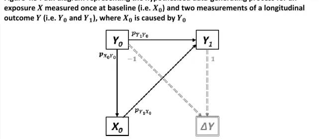
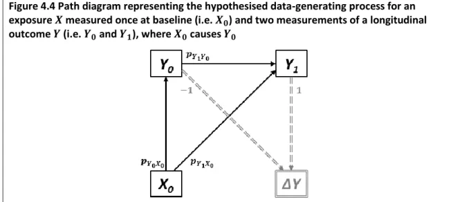
exposure 𝑿 measured once at baseline (i.e. 𝑿𝟎) and two measurements of a longitudinal outcome 𝒀 (i.e. 𝒀𝟎 and 𝒀𝟏), where 𝑿𝟎 is caused by 𝒀𝟎 ... 48 Figure 4.4 Path diagram representing the hypothesised data-generating process for an

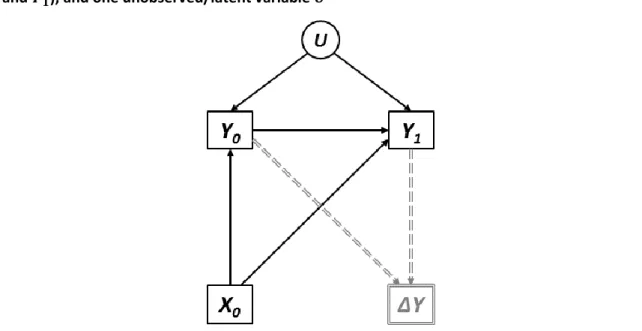
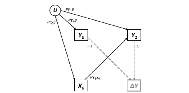
exposure 𝑿 measured once at baseline (i.e. 𝑿𝟎) and two measurements of a longitudinal outcome 𝒀 (i.e. 𝒀𝟎 and 𝒀𝟏), where 𝑿𝟎 causes 𝒀𝟎 ... 50 Figure 4.5 DAG representing the hypothesised data-generating process for an exposure 𝑿 measured once at baseline (i.e. 𝑿𝟎), two measurements of a longitudinal outcome

(18)

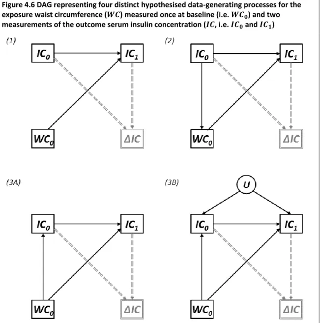
Figure 4.6 DAG representing four distinct hypothesised data-generating processes for the exposure waist circumference (𝑾𝑪) measured once at baseline (i.e. 𝑾𝑪𝟎) and two measurements of the outcome serum insulin concentration (𝑰𝑪, i.e. 𝑰𝑪𝟎 and 𝑰𝑪𝟏) ... 54 Figure 4.7 Path diagram representing Lord’s Paradox (147) ... 59 Figure 4.8 Path diagram representing the analysis of change as depicted by Kim, Y. and

P.M. Steiner (148) ... 61 Figure 5.1 DAG depicting the hypothesised data-generating process for two

measurements of a time-varying exposure 𝑿 (i.e. 𝑿𝟎 and 𝑿𝟏) and one outcome 𝒀65 Figure 5.2 Path diagrams depicting the two standard regression models that would be

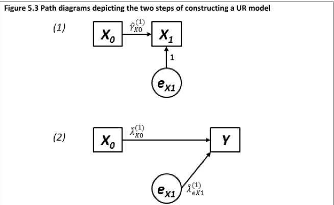
constructed to estimate the total causal effect of each of 𝑿𝟎 and 𝑿𝟏 on 𝒀 (i.e. Equation 5.1 and Equation 5.2, respectively) ... 66 Figure 5.3 Path diagrams depicting the two steps of constructing a UR model... 66 Figure 5.4 Directed acyclic graph (DAG) depicting the hypothesised data-generating

process for two measurements of a time-varying exposure 𝑿 (i.e. 𝑿𝟎 and 𝑿𝟏), one outcome 𝒀, and one baseline confounder 𝑴 ... 70 Figure 5.5 Path diagrams depicting the two standard regression models that would be

constructed to estimate the total causal effect of each of 𝑿𝟎 and 𝑿𝟏 on 𝒀 in the presence of a baseline confounder 𝑴 (i.e. Equation 5.5 and Equation 5.6,

respectively) ... 71 Figure 5.6 Path diagrams depicting the two steps of constructing a UR model in the

presence of a baseline confounder 𝑴 ... 72 Figure 5.7 Directed acyclic graph (DAG) depicting the hypothesised data-generating

process for two measurements of a time-varying exposure 𝑿 (i.e. 𝑿𝟎 and 𝑿), one outcome 𝒀, and two measurements of a time-dependent confounder 𝑴 (i.e. 𝑴𝟎 and 𝑴𝟏) ... 73 Figure 5.8 Path diagrams depicting the two standard regression models that would be

constructed to estimate the total causal effect of each of 𝑿𝟎 and 𝑿𝟏 on 𝒀 in the presence of time-dependent confounders 𝑴𝟎 and 𝑴𝟏 (i.e. Equation 5.9 and Equation 5.10, respectively) ... 74 Figure 5.9 Path diagrams depicting the three steps of constructing a UR model in the

presence of time-dependent confounders 𝑴𝟎 and 𝑴𝟏 ... 75 Figure 5.10 DAG depicting the hypothesised data-generating process for 𝑻 measurements

of a time-varying exposure 𝑿 (i.e. 𝑿𝟎, 𝑿𝟏, … , 𝑿𝑻 − 𝟏) and one outcome 𝒀. ... 77 Figure 5.11 DAG depicting the hypothesised data-generating process for 𝑻 measurements

of a time-varying exposure 𝑿 (i.e. 𝑿𝟎, 𝑿𝟏, … , 𝑿𝑻 − 𝟏), one outcome 𝒀, and one baseline confounder 𝑴 ... 78 Figure 5.12 DAG depicting the hypothesised data-generating process for 𝑻 measurements

of a time-varying exposure 𝑿 (i.e. 𝑿𝟎, 𝑿𝟏, … , 𝑿𝑻 − 𝟏), one outcome 𝒀, and 𝑻 measurements of a time-varying exposure 𝑴 (i.e. 𝑴𝟎, 𝑴𝟏, … , 𝑴𝑻 − 𝟏) ... 79 Figure 5.13 Violin plots comparing the standard errors (SEs) associated with equivalent

coefficients estimated in standard regression vs. UR models ... 81 Figure 6.1 DAG representing the data-generating process for the variables sex (𝑺), obesity

(19)

Figure 6.2 Obesity prevalence in the simulated population under Interventions 1 through 6, compared to the natural history ... 91 Figure 6.3 Diabetes prevalence in the simulated population under Interventions 1 through

6, compared to the natural history ... 92 Figure 6.4 Proportion of individuals in the simulated population with each combination of

sex, obesity status, and diabetes status under Interventions 1 through 6, compared to the natural history ... 93 Figure 6.5 DAGs representing three hypothesised data-generating processes at time 𝒕 for the time-varying variables obesity (𝑶) and diabetes (𝑫) ... 97 Figure 6.6 Natural history of obesity and diabetes prevalence for each of the

autocorrelation structures modelled using the g-formula, compared to the true natural history ... 100 Figure 6.7 Natural history of the cross-sectional prevalence of sex, obesity, and diabetes,

for each of AS1 through AS3 modelled using the g-formula, compared to the true natural history ... 101 Figure 6.8 Counterfactual histories of obesity and diabetes prevalence under Intervention

1 for each of AS1 through AS3 modelled using the g-formula, compared to the true counterfactual history ... 102 Figure 6.9 Natural history of obesity and diabetes prevalence for each of AS1 through AS3

modelled using microsimulation, compared to the true natural history ... 105 Figure 6.10 Natural history of the cross-sectional prevalence of sex, obesity, and diabetes,

for each of AS1 through AS3 modelled using microsimulation, compared to the true natural history ... 106 Figure 6.11 Counterfactual histories of obesity and diabetes prevalence under

Intervention 1 for each of AS1 through AS3 modelled using microsimulation, compared to the true counterfactual history ... 107 Figure A.1 DAGs from which multivariate normal data were simulated to demonstrate the

degree of inferential bias that might be introduced by a change-score analysis .. 124 Figure A.2 DAGs from Figure A.1, with an additional unmeasured baseline confounder 𝑼𝟐 ... 125 Figure B.1 Directed acyclic graph from which multivariate normal data were simulated to demonstrate standard error reduction in UR models ... 143 Figure C.1 Proportion of individuals in the simulated population with each combination of

sex, obesity status, and diabetes status at every time point ... 150 Figure C.2 Probabilities of becoming and remaining obese in the simulated population at every time point ... 151 Figure C.3 Probabilities of becoming and remaining diabetic in the simulated population

at every time point ... 151 Figure C.4 Obesity and diabetes prevalence in the simulated population compared to the Health Survey for England (HSE, years 1994-2004) ... 152 Figure C.5 Probability of becoming obese at time 𝒕 for Interventions 1 through 6,

compared to those of the natural history ... 160 Figure C.6 Probability of remaining obese at time 𝒕 for Interventions 1 through 6,

(20)

Figure C.7 Probability of becoming diabetic at time 𝒕 for Interventions 1 through 6, compared to those of the natural history ... 162 Figure C.8 Probability of remaining diabetic at time 𝒕 for Interventions 1 through 6,

compared to those of the natural history ... 163 Figure C.9 Counterfactual histories of obesity and diabetes prevalence under Intervention

2 for each of AS1 through AS3 modelled using the g-formula, compared to the true counterfactual history ... 175 Figure C.10 Counterfactual histories of obesity and diabetes prevalence under

Intervention 3 for each of AS1 through AS3 modelled using the g-formula,

compared to the true counterfactual history ... 176 Figure C.11 Counterfactual histories of obesity and diabetes prevalence under

Intervention 2 for each of AS1 through AS3 modelled using microsimulation, compared to the true counterfactual history ... 191 Figure C.15 Counterfactual histories of obesity and diabetes prevalence under

Intervention 6 for each of AS1 through AS3 modelled using microsimulation, compared to the true counterfactual history ... 195

(21)

List of abbreviations

ABM Agent-based model

ANCOVA Analysis of covariance

BMI Body mass index

CRCT Conditionally randomised controlled trial DAG Directed acyclic graph

GDP Gross domestic product

IPTW Inverse probability of treatment weight(ing) MSAS Minimally sufficient adjustment set

MSM Microsimulation model

NHANES National Health and Nutrition Examination Survey OLS Ordinary least squares

RCT Randomised controlled trial

RTM Regression to the mean

SE Standard error

SNM Structural nested model TCE Total causal effect UR Unexplained residual(s)

(22)

(23)

Chapter 1 Introduction

1.1 Introduction

Estimating the causal effect of a particular factor or event (an ‘exposure’1_{) on a subsequent}

factor or event (an ‘outcome’) is not a trivial task. Causation is a concept for which most (if not all) human beings have an intuitive understanding. Nevertheless, it is a complex phenomenon which may be difficult to even articulate. Despite thousands of years of philosophical

discourse, there exists very little consensus as to what it is, how it can be defined, and – perhaps most importantly for researchers – how it can be inferred within practical research applications (7-15). Prominent theories of causation include the regularity, counterfactual, probabilistic, agency and interventionist, and mechanistic theories (16), though no single account may be considered universal because each is subject to counterexamples (17). The counterfactual framework has risen to prominence as the dominant paradigm for testing and evaluating causal claims in many disciplines; this is likely due to both its conceptual simplicity and its recent mathematical formalisation in the form of directed acyclic graphs (DAGs).2_{However, in spite of its prominence, there exist many (purportedly causal) methods}

which have not been examined through this lens. This PhD thesis explores how counterfactual thinking, encoded in the language of DAGs, may be integrated into established methods for longitudinal data analysis; this thesis also seeks to demonstrate the advantages of doing so, though focus on the counterfactual framework is not intended to imply its superiority over any other causal framework. The contexts considered are primarily health- and epidemiology-focused, but the analyses performed have applicability to other domains.

Population-level health patterns emerge from a complex, dynamic, and multi-layered system, in which a multitude of different interrelationships operate (21). Estimating causal effects in this context requires somehow accounting for all potential non-causal associations and biases which may distort the association of interest (2). Historically, a ‘top-down’ approach has been implemented to control such complexities and minimise biases via study design (e.g. case-control studies, randomised case-controlled trials). However, in the era of ‘big data’, we are increasingly awash with large and complex datasets from the many systems and technologies that routinely record information on individual experiences. Big data offers much promise for

1_{The term ‘treatment’ is often used interchangeably with ‘exposure’, particularly in medical- and}

health-related contexts (6).

2_{This framework is substantively very similar to the ‘potential outcomes’ framework introduced by Jerzy}

Neyman in 1923 (18) and more extensively developed and popularised by Donald Rubin from 1974 (19, 20), though the two frameworks employ different terminology and possess other subtle differences.

(24)

understanding causal processes, but it does not in and of itself eliminate any of the classical challenges and data quality issues associated with observational data, such as missing or incomplete data and measurement error (22). Neither does big data eliminate the need for a priori subject matter knowledge, since any association may reach the threshold of ‘statistical significance’ given sufficiently large sample sizes. To fully exploit the potential of big data, robust methods for evaluating causal relationships are needed which emphasise

understanding data-generating processes from the bottom up.

Longitudinal data in particular form a large proportion of the new and emerging forms of data in the digital age. For instance, smartphone apps are able to continuously track and collect data relating to location and activity levels. Hospital records constitute another example, which may additionally be linked to general practice and pharmacy records to create a more comprehensive picture of an individual’s interaction with health services over time. Traditional forms of data collection like cross-sectional surveys are inherently longitudinal, since even data which are collected or measured at the same time are likely to have an implicit time ordering. This is because the time at which a variable is measured implies nothing about the time at which its value became manifest. For example, a cross-sectional survey may contain information on individuals’ biological sex and their weight, but these variables nevertheless have a clear temporal ordering – sex becomes fixed at the time of conception, whereas weight represents an accumulation of infinitesimal changes throughout the life course and whose value only becomes manifest at the time it is measured. However, the term ‘longitudinal’ is typically applied to data for which there exist multiple measurements of one or more variables, and this is the meaning we adopt throughout. Such data are explicitly longitudinal, and are of particular interest to epidemiologists and data scientists as they allow for changes to be quantified and examined. A key focus of life course epidemiology, for instance, is to identify and quantify important periods of change or growth in an exposure, and to evaluate their effect on subsequent outcomes (23, 24).

Longitudinal data may be conceptualised both as exposures and as outcomes, but across all contexts they present analytical challenges for causal inference over and above those of cross-sectional data. This thesis explores some of those challenges in the context of three statistical- and simulation-based methods for assessing causal relationships, and demonstrates the insights that DAGs and the counterfactual framework can bring to causal analyses.

1.2 Aims and objectives

As outlined previously, the aim of this PhD thesis is to explore how DAGs can be integrated into established methods for longitudinal data analysis, and to illustrate the benefits of doing so. To this end, three specific statistical- and simulation-based methods are considered, all of which relate to distinct longitudinal scenarios but which are connected via the fact that they are purportedly used for estimating causal relationships.

(25)

As broad objectives, DAGs will be used to depict the longitudinal context in which each method is deployed; the principles of graphical model theory will be applied in order to identify how each method should be employed to robustly estimate causal effects; and the potential biases which result from failing to consider each method within a robust causal framework will be identified and explored.

1.3 Thesis overview

Chapter 2 provides background literature related to the counterfactual framework for causal inference, and demonstrates how this framework has been formalised mathematically in the language of DAGs. The aim of this chapter is to provide sufficient information related to the concepts and vocabulary which are necessary for understanding the contents of the remainder of the thesis.

Chapter 3 expands on Chapter 2 by introducing several methods for estimating causal effects in longitudinal data, some of which are based on DAGs but many of which are not. The utility of using DAGs to inform causal analyses is demonstrated through specific examples.

Additionally, a critical comparison of statistical methods and individual-based simulation methods is provided, since both have been recognised as useful tools for evaluating

counterfactual contrasts. This provides a foundation for understanding the contexts in which the methods considered in the remainder of the thesis may be used, as well as understanding some of the potential strengths and weaknesses of these methods.

Each of the next three chapters uses DAGs to examine a particular method for estimating causal effects in longitudinal data. The methods are both statistical- and simulation-based, and each method relates to a different longitudinal scenario.

Chapter 4 uses DAGs to consider the analysis of change – a topic which has historically been a matter of much disagreement but which has rarely been examined within the framework of DAGs. This context involves quantifying the relationship between a single exposure and subsequent ‘change’ in a longitudinal outcome. In this chapter, the concept of ‘change’ is considered within a formal causal framework, in order to demonstrate the analytical strategies most compatible with analysing ‘change’ and the problems which may arise by failing to consider underlying causal structures and data-generating processes.

Chapter 5 uses DAGs to consider regression with ‘unexplained residuals’ – a method which was introduced to circumvent some of the difficulties associated with estimating causal effects in longitudinal settings but which was never extended to address confounding. This context involves quantifying the relationship between separate measurements of a longitudinal exposure and a subsequent outcome. In this chapter, DAGs are used to illustrate why the method works in the absence of any confounding, and to provide the principles on which the method may be extended robustly to account for confounding by both fixed and time-varying covariates.

(26)

Chapter 6 uses DAGs to consider microsimulation modelling – a simulation method often used to estimate counterfactual quantities for policy evaluation and which shares many similarities with the statistical ‘g-formula’. This context involves quantifying the relationship between multiple measurements of a longitudinal exposure and a subsequent outcome. In this chapter, DAGs are used to consider the parallels between the data-generating processes they represent and those which are modelled using microsimulation, and the importance of faithfully

modelling data-generating processes from the bottom up in order to make causal inferences. Chapter 7 summarises the findings and implications of all chapters, including their

contributions to the literature. It additionally discusses the limitations of the research

contained in the thesis, and offers suggestions for future research of this kind. Potential areas for future research are outlined.

(27)

Chapter 2 Background

2.1 Introduction

Epidemiological research relies primarily on the counterfactual theory of causation for testing and evaluating causal claims. Counterfactual reasoning underpins randomised controlled trials, long considered to be the superior and most robust method for demonstrating causal effects. However, the counterfactual framework has also been formalised in the language of DAGs, which provide a rigorous mathematical framework for causal analyses and the identification of causal effects in non-randomised contexts.

Chapter 2 provides a comprehensive introduction to the counterfactual framework for exposures which are both time-fixed and time-varying; of fundamental importance is the concept of exchangeability, which allows for the identification of causal effects in this

framework. This chapter also introduces DAGs, and illustrates their utility in identifying causal effects for time-fixed and time-varying exposures. Since this thesis explores how DAGs may be integrated into established methods for longitudinal data analysis, the purpose of this chapter is to provide sufficient information related to the relevant concepts and vocabulary which are necessary for understanding the remainder of this thesis.

2.1.1 Chapter overview

A general chapter overview is provided below.

In Section 2.2, we distinguish between time-fixed and time varying variables, and consequently define what it means for an exposure to be either time-fixed (§2.2.1) or time-varying (§2.2.2). In Section 2.3, we introduce the counterfactual framework for causal inference. We use specific examples to demonstrate how this framework conceptualises individual-level causal effects for both time-fixed (§2.3.1.1) and time-varying (§2.3.1.2) exposures. We additionally highlight a crucial concept in counterfactual causation – exchangeability (§2.3.2).

In Section 2.4, we discuss how randomisation may be used to identify average causal effects for both time-fixed (§2.4.1) and time-varying (§2.4.2) exposures. We highlight the difference between unconditional and conditional exchangeability in each context.

In Section 2.5, we introduce graphical causal models, with particular focus given to DAGs (§2.5.2). We illustrate how DAGs may be used to identify causal effects for both time-fixed (§2.5.3) and time-varying (§2.5.4) exposures by emulating randomisation.

(28)

2.2 Time-fixed versus time-varying variables

A variable is considered to be time-fixed if it occurs only once (e.g. a one-dose vaccine, birthweight), does not change over time (e.g. sex, BRCA1/BRCA2 genes (25)), or evolves over time in a deterministic way (e.g. age, time since treatment) (26). Very few time-fixed variables exist over the entire lifecourse, but over shorter periods of time certain variables may be reasonably conceptualised and/or treated as time-fixed. For example, height changes substantially over the lifecourse, though remains relatively fixed throughout middle-age. In contrast, a variable is considered to be time-varying if it occurs multiple times (e.g. a multi-dose vaccine) or changes over time (e.g. smoking status, blood sugar) (26). Such variables form the majority of those of interest in epidemiological applications, though the complexity of dealing with variables of this type means that they are often ‘reclassified’ as time-fixed by defining their values at a particular point in time. For example, height at age three and height at age five could be considered as two distinct time-fixed variables.

2.2.1 Time-fixed exposures

We use the term time-fixed exposure to refer to an exposure whose effect on an outcome of interest is only being considered at a single point in time. For example, an epidemiologist might consider what effect obesity at age fifteen has on the risk of depression at age twenty. Although obesity is a time-varying variable, it is considered a time-fixed exposure in this context because its effect is only being considered at the specific age of fifteen.

2.2.2 Time-varying exposures

We use the term time-varying exposure to refer to an exposure whose effect on an outcome is being considered at multiple points in time. For example, an epidemiologist might consider what effect obesity at ages ten, fifteen, and eighteen has on the risk of depression at age twenty. A sequence of exposures such as this is often referred to an exposure (or treatment) regime.

2.3 The counterfactual framework for causal inference

Here, we introduce the basic concepts of, and the intuition behind, the counterfactual

framework for causal inference. This framework is most easily conceptualised in the context of individual-level causal effects, and so we define such effects for both time-fixed (§2.3.1.1) and time-varying (§2.3.1.2) exposures. We additionally highlight the key concept of exchangeability (§2.3.2) and the so-called ‘fundamental problem of causal inference’ for the identification of individual-level causal effects (§2.3.3).

2.3.1 Individual-level causal effects

2.3.1.1 For time-fixed exposures

The counterfactual framework states that an event 𝑋 (i.e. a time-fixed exposure) may be considered a cause of an event 𝑌 if, contrary to fact, had 𝑋 not occurred then 𝑌 would not

(29)

have occurred (16, 27). As an example (adapted from (27)), we can imagine that an individual, Mary, is driving to work and comes to a fork in the road. She chooses to go left (i.e. event 𝑋) and subsequently arrives late for work (i.e. event 𝑌). Upset, Mary declares ‘I should have gone right instead!’ What her statement implies is that her decision to go left at the fork in the road caused her to be late for work because, had she gone right instead (i.e. event ‘not 𝑋’), she would arrived on time (i.e. event ‘not 𝑌’). Of course, there is no way to prove her statement, as doing so would require Mary to simultaneously go both left and right and then observe the outcome under each condition, in order to guarantee that the effect cannot be attributed to any other factor that differed between the drives. Nevertheless, this example demonstrates the intuition of (and utility behind) conceptualising causal effects as counterfactual contrasts between two scenarios that are equivalent in every way except for the putative causal factor of interest.

2.3.1.2 For time-varying exposures

The counterfactual framework – although more frequently conceptualised in the context of time-fixed exposures – can also be naturally extended to time-varying exposures. To this end, we consider a scenario involving two events 𝑋0 and 𝑋1 (i.e. a time-varying exposure). The events 𝑋0 and 𝑋1 may be considered a joint cause of an event of 𝑌 if, contrary to fact, had at least one of 𝑋0 or 𝑋1 not occurred then 𝑌 would not have occurred (26). As an example, we can imagine that Mary takes two doses of antibiotics to treat a chest infection (i.e. events 𝑋0 and 𝑋1, respectively), which clears up (i.e. event 𝑌) after the second dose. We may conclude the two doses of antibiotics are a joint cause of clearing Mary’s chest infection if there exists a counterfactual scenario in which Mary did not take at least one of the doses and her chest infection did not clear. For example, if Mary did not take the second dose of antibiotics (i.e. event ‘not 𝑋1’) and her chest infection persisted (i.e. event ‘not 𝑌’), we could conclude that the two doses are a joint cause of her chest infection clearing. However, if Mary’s chest infection cleared regardless of whether she took each dose of antibiotics (i.e. if all counterfactual scenarios resulted in the same outcome), the clearing cannot be attributed to the antibiotic regime.

2.3.2 Exchangeability

Exchangeability is a fundamental concept in counterfactual causation. In this framework, a causal effect is defined in terms of a comparison between two units of analysis which are in all ways equivalent except for the putative causal factor of interest – in other words, two units of analysis which are exchangeable.

2.3.3 The ‘fundamental problem of causal inference’

The so-called ‘fundamental problem of causal inference’ (28) is that individual-level causal effects cannot ever be identified because it is impossible to observe an individual subjected to different values of the putative causal factor simultaneously. In other words, it is impossible to

(30)

view the unrealised counterfactual scenario(s) and therefore impossible to achieve exchangeability.

2.4 Using randomisation to identify average causal effects

Although identification of individual-level causal effects is generally agreed to be impossible within the counterfactual framework, identification of average causal effects is possible and forms the basis of a great deal of epidemiological causal inference (6). Average causal effects may be identified by creating exchangeable groups of individuals and comparing their average outcomes. This is often achieved through randomisation (29, 30).

2.4.1 Average causal effects for time-fixed exposures

To demonstrate the principle of using randomisation to identify the average causal effect for a time-fixed exposure, we consider a specific example involving the effect of chemotherapy versus radiotherapy on two-year survival amongst breast cancer patients. We illustrate how both unconditionally and conditionally exchangeable groups of individuals may be created by randomisation.

2.4.1.1 Exchangeability

2.4.1.1.1Unconditional exchangeability

Epidemiologists have long considered the randomised controlled trial (RCT) to be the ‘gold standard’ for demonstrating causality because, if implemented correctly, it guarantees unconditional exchangeability (31). An RCT in our example context might involve randomly assigning each patients to receive either chemotherapy and radiotherapy, and then comparing the average outcome for each treatment group.

In this situation, the group who received chemotherapy is unconditionally exchangeable with the group who received radiotherapy. This is because randomisation ensures that the outcome is equally likely in both groups prior to the intervention, and so a simple comparison of the average outcome for each group after the intervention is sufficient to identify an average causal effect (32). In other words, those who received chemotherapy, had they instead received radiotherapy, would have experienced the same average outcomes as those who actually did receive radiotherapy (6), i.e. they are unconditionally exchangeable.3

2.4.1.1.2Conditional exchangeability

We could alternately consider a conditionally randomised controlled trial (CRCT), in which each patient is randomly assigned to receive either chemotherapy or radiotherapy based on

3_{If there exists differential loss to follow-up, then exchangeability may not be ensured by this process}

(33, 34). However, this is an additional complexity which we do not cover here, since our purpose is simply to illustrate the conceptual rationale behind such designs.

(31)

their initial cancer stage. For example, individuals in stage IV are randomised to receive chemotherapy with a higher probability than radiotherapy.

Here, a simple comparison of the average outcome for each treatment group cannot be assumed sufficient, as any difference in two-year survival might be attributable to the fact that the chemotherapy group has, on average, a worse prognosis at the beginning of the study. Nevertheless, we are still able to identify an average causal effect by comparing the average two-year survival between those who received chemotherapy and those who received radiotherapy among individuals who had the same initial cancer stage. Thus, within each subgroup of cancer stage, those who received chemotherapy, had they instead received radiotherapy, would have experienced the same average outcomes as those who actually did receive radiotherapy (6). The two treatment groups are conditionally exchangeable, i.e. they are exchangeable conditional on initial cancer stage.

2.4.2 Average causal effects for time-varying exposures

To demonstrate the principle of using randomisation to identify an average causal effect for a time-varying exposure, we return to the example from Section 2.3.1.2 involving the use of antibiotics to clear a chest infection, in which a dose of antibiotics may be prescribed at the point of initial diagnosis or at a subsequent follow-up visit.

We illustrate in this context how unconditionally and conditionally exchangeable groups of individuals may be manufactured by sequential randomisation.

2.4.2.1 Exchangeability

2.4.2.1.1(Sequential) unconditional exchangeability

An RCT in our example context might involve randomly assigning each patient to receive each dose of antibiotics. This is referred to as ‘sequential randomisation’ (26) because patients are randomised at each time point. In this way, we create four treatment groups – those who received two doses, no doses, only the first dose, or only the second dose.

The proportion of people whose infections subsequently cleared in each of the treatment groups may then be directly compared. The process of sequential randomisation ensures that the outcome is equally likely in all groups prior to treatment both at the point of diagnosis and at the point of follow-up. Thus, a simple comparison of the average outcome for each group after the final intervention is sufficient to identify an average causal effect. For example, those who received both doses of antibiotics, had they instead received one of the other dosing regimes, would have experienced the same average outcomes as those who actually did receive those other dosing regimes (6), i.e. they are unconditionally exchangeable. 2.4.2.1.2(Sequential) conditional exchangeability

By contrast, a CRCT in our example context might instead involve randomly assigning each patient to receive each dose of antibiotics based on the severity of their infection at the time.

(32)

For example individual who are initially judged to have more severe infections may be randomised to receive the first dose of antibiotics with a higher probability than those with less severe infections. Similarly, individuals with more severe infections at the follow-up visit may be randomised to receive the second dose with a higher probability.

Because each treatment group (i.e. those who received two doses, no doses, only the first dose, or only the second dose) is likely to have a different average outcome prognosis as a result of the way in which individuals were randomised, they cannot be directly compared. Moreover, we cannot even identify an average causal effect by comparing the proportion cleared chest infections among individuals who had the same infection severity at both time points, because infection severity at the second time point is itself affected by whether or not an individual received the first dose of antibiotics (i.e. infection severity is not randomised). However, within subgroups defined by initial infection severity, receipt of the first dose of antibiotics, and follow-up infection severity, those who received the second dose of antibiotics, had they instead not received the second dose of antibiotics, would have experienced the same distribution of outcomes as those who actually did not receive the second dose. The average outcome for each of the treatment groups may then be compared within levels of baseline and follow-up infection severity because they are (sequentially) conditionally exchangeable, i.e. they are exchangeable at each time point conditional on current infection severity.

We will return to this concept in Section 2.5.4, where we present a clearer graphical depiction of this issue (§2.5.4.1) and the challenges associated with identifying casual effects in

sequentially randomised contexts (§2.5.4.2).

2.5 Using DAGs to identify average causal effects

For situations in which (C)RCTs are either infeasible (e.g. for extremely rare diseases),

impractical (e.g. for complex and/or costly interventions), and/or unethical (e.g. for potentially deadly or otherwise harmful exposures), epidemiologists must rely on observational, non-randomised data. However, the average causal effect of an exposure on an outcome may still be identified by using the principles of graphical model theory to emulate exchangeability. In this section, we give a brief introduction to graphical causal models and DAGs, and illustrate how they encode counterfactual statements for both time-fixed and time-varying exposures.

2.5.1 Graphical causal models

Modern causal models trace their roots to 1918, with Sewall Wright’s invention of path analysis (35, 36). They also have origins in structural equation models (SEMs), which represent groups of causally related variables (both observed and latent) as systems of simultaneous linear equations (37). However, both were subsumed at the beginning of the twenty-first century under the framework of nonparametric causal models by Judea Pearl in his seminal book Causality (38).

(33)

These models are typically represented graphically (hence ‘graphical causal models’4_{) and}

consist of two fundamental components: 1. A set of variables (i.e. ‘nodes’); and 2. A set of arrows (i.e. ‘arcs’ or ‘edges’).

Any two variables in the graph may be connected by an arrow (e.g. 𝐴 → 𝐵), which means that the first variable (𝐴) exerts a direct causal effect on the second (𝐵) for at least one member of the population (39). A variable may be either endogenous (i.e. having at least one direct cause represented in the graph), or exogenous (i.e. having no direct causes represented in the graph). However, the graph makes no assumptions about the distribution of the variables, nor does it imply or constrain either the magnitude or functional form of the causal effects (27, 39).

Two examples of graphical causal models are provided in Figure 2.1. By convention, observed and/or measured variables are denoted by rectangles, whereas unmeasured and/or

unobserved (i.e. latent) variables are denoted by ovals. We also adopt the convention that time flows from left to right (6).

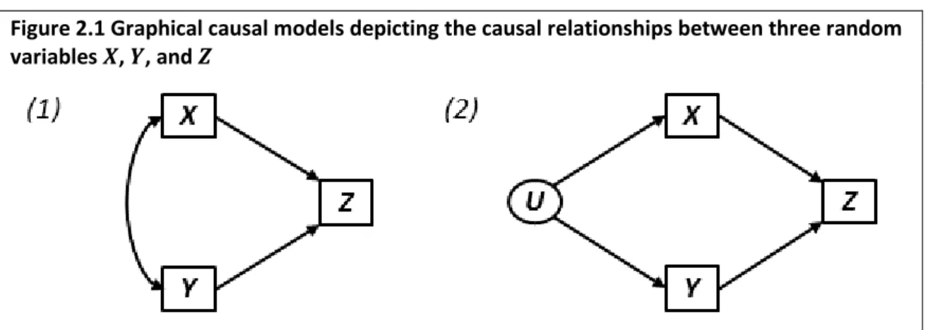
Figure 2.1 Graphical causal models depicting the causal relationships between three random variables 𝑿, 𝒀, and 𝒁

Observed and/or measured variables are depicted in rectangular boxes, and latent variables are depicted in ovals. In panel (1), 𝑋 and 𝑌 cause one another. In panel (2), 𝑋 and 𝑌 are caused by the unobserved variable 𝑈.

The graphical causal model in panel (1) of Figure 2.1 depicts the causal relationships between the variables 𝑋, 𝑌, and 𝑍; the graph implies that both 𝑋 and 𝑌 are direct causes of 𝑍, and that

𝑋 and 𝑌 cause each other. The graphical causal model in panel (2) of Figure 2.1 is very similar to that in panel (1), but instead depicts 𝑋 and 𝑌 as being caused by the unobserved variable 𝑈, which is the source of their mutual dependency.

The graph in panel (2) is a particular type of graphical causal model – a directed acyclic graph.

4_{Graphical causal models may alternately be referred to as ‘causal diagrams’ (6), ‘graphical models’}

(34)

2.5.2 Directed acyclic graphs (DAGs)

Directed acyclic graphs (DAGs) represent a special subset of graphical causal models, as they form the foundation on which modern statistical causal inference methods are based. A DAG is a graphical causal model in which all arrows are unidirectional (hence ‘directed’). Moreover, no variable can indirectly cause itself (hence ‘acyclic’) (6, 39). As identified previously, the graphical causal model in panel 1 of Figure 2.1 is not a DAG because there exists a bidirectional arrow between 𝑋 and 𝑌, whereas the graphical causal model in panel 2 of Figure 2.1 is a DAG because the bidirectional arrow has been replaced by two unidirectional arrows emanating from the common cause 𝑈.

DAGs encode qualitative causal assumptions about the data-generating process in the

population (39), i.e. the process by which any endogenous value in the graph obtains its value. Given information on all exogenous variables in a DAG, the values of any endogenous variable can be identified. In Figure 2.2, for example, if we know the values of 𝐴 and 𝐵 (the exogenous variables, which have no causes in the graph) we are able to identify the value of 𝐶, as it depends only on 𝐴 for its value. Similarly, we are able to identify the values of all other endogenous variables 𝐷, 𝐸, and 𝐹, as they depend only on other variables in the graph. Figure 2.2 DAG depicting the data-generating process for the six random variables 𝑨, 𝑩, 𝑪,

𝑫, 𝑬, and 𝑭

2.5.2.1 Key terminology

Kinship terminology is often employed to describe the relationships between variables in a DAG (39). For example, the variables which are directly caused by a given variable are called its children (e.g. 𝐶 and 𝐷 are children of 𝐴 in Figure 2.2), and all variables which are directly or indirectly caused by a given variable are called its descendants (e.g. 𝐶, 𝐷, 𝐸, and 𝐹 are

descendants of 𝐴 in Figure 2.2). Conversely, the variables which directly cause a given variable are called its parents (e.g. 𝐶 and 𝐷 are parents of 𝐸 in Figure 2.2), and all variables which directly or indirectly cause a given variable are called its ancestors (e.g. 𝐴, 𝐶, and 𝐷 are ancestors of 𝐸 in Figure 2.2).

A path is a sequence of arrows connecting two variables, regardless of the orientation of those arrows; there may be multiple paths connecting any two nodes in the graph (39). For example,

Statistical and simulation-based modelling approaches for causal inference in longitudinal data: Integrating counterfactual thinking into established methods for longitudinal data analysis