Agent-Based Model Calibration using
Machine Learning Surrogates
Francesco Lamperti
Andrea Roventini
Amir Sani
EDITORIAL BOARD
Chair: Xavier Ragot (Sciences Po, OFCE)
Members: Jérôme Creel (Sciences Po, OFCE), Eric Heyer(Sciences Po, OFCE), Lionel Nesta (Université Nice Sophia Antipolis), Xavier Timbeau (Sciences Po, OFCE)
CONTACT US OFCE
10 place de Catalogne | 75014 Paris | France Tél. +33 1 44 18 54 87
www.ofce.fr
WORKING PAPER CITATION
This Working Paper:
Francesco Lamperti, Andrea Roventini, et Amir Sani, Agent-Based Model Calibration using Machine Learning Surrogates, Sciences Po OFCE Working Paper, n°09, 2017-03-30.
Downloaded from URL : www.ofce.sciences-po.fr/pdf/dtravail/WP2017-09.pdf
DOI - ISSN
ABOUT THE AUTHORS
Francesco Lamperti Scuola Superiore Sant’Anna, Pisa, Italy. Corresponding author.
Email Address:[email protected]
Andrea Roventini Scuola Superiore Sant’Anna, Pisa, Italy. Also OFCE, Sciences Po, Paris, France.
Email Address: andrea.roventini<at>santannapisa.it
Amir Sani Université Panthéon-Sorbonne and CNRS, Paris, France Email Address:[email protected]
ABSTRACT
Taking agent-based models (ABM) closer to the data is an open challenge. This paper explicitly tackles parameter space exploration and calibration of ABMs combining supervised machine-learning and intelligent sampling to build a surrogate meta-model. The proposed approach provides a fast and accurate approximation of model behaviour, dramatically reducing computation time. In that, our machine-learning surrogate facilitates large scale explorations of the parameter-space, while providing a powerful filter to gain insights into the complex functioning of agent-based models. The algorithm introduced in this paper merges model simulation and output analysis into a surrogate meta-model, which substantially ease ABM calibration. We successfully apply our approach to the Brock and Hommes (1998) asset pricing model and to the “Island” endogenous growth model (Fagiolo and Dosi, 2003). Performance is evaluated against a relatively large out-of-sample set of parameter combinations, while employing different user-defined statistical tests for output analysis. The results demonstrate the capacity of machine learning surrogates to facilitate fast and precise exploration of agent-based models’ behaviour over their often rugged parameter spaces.
KEY WORDS
Agent based model; calibration; machine learning; surrogate; meta-model. JEL
1
Introduction
This paper proposes a novel approach to model calibration and parameter space exploration in agent-based models (ABM), combining supervised machine learning and intelligent sampling in the design of a novel surrogate meta-model.
Agent-based models deal with the study of socio-ecological systems that can be properly conceptualized through a set of micro and macro relationships. One problem with this frame-work is that the relevant statistical properties for variables of interest are a priori unknown, even to the modeler. Such properties emerge indeed from the repeated interactions among ecologies of heterogeneous, boundedly-rational and adaptive agents.1 As a result, the dynamic properties of the system cannot be studied analytically, the identification of causal mechanisms is not always possible and interactions give rise to the emergence of relationships that cannot simply be deduced by aggregating those of micro variables (Anderson et al., 1972, Tesfatsion and Judd, 2006, Grazzini, 2012, Gallegati and Kirman,2012). This raises the issue of finding appropriate tools to investigate the emergent behavior of the model with respect to different parameter settings, random seeds, and initial conditions (see also Lee et al., 2015). Once this search is successful, one can safely move to calibration, validation and, finally, employ the model for policy exercises (more on that inFagiolo and Roventini,2017). Unfortunately, this procedure is hardly implementable in practice, notably due to large computation times.
Indeed, many ABMs simulate the evolution of complex systems with a large number of parameters for a relatively many time steps. In a calibration setting, this rich expressiveness results in a “curse of dimensionality” that lends to an exponential number of critical points along the parameter space, with multiple local maxima, minima and saddle points, which negatively impact the performance of gradient-based search procedures. Indeed, even for small models, exploring the behavior of the model through all possible parameter combinations (a full factorial exploration) is practically impossible, even employing multi-objective optimization procedures such as multimodel optimization or niching (for a review, see e.g.Li et al.,2013;Wong,2015).2 However, if a model is to be used by policy makers or regulators, it must provide timely insights into the problem. As a result, gaining an intuition from models with rich expressiveness, but computationally expensive evaluations, is of limited practical interest.
Traditionally, three computationally expensive steps are involved in ABM calibration; run-ning the model, measuring calibration quality and locating parameters of interest. As remarked inGrazzini et al.(2017), such steps account for more than half of the time required to estimate ABMs, even for extremely simple models. Recently, Kriging (also known as Gaussian processes) has been employed to build surrogate meta-models of ABMs (Salle and Yildizoglu,2014;Dosi
1In the last two decades a variety of ABM have been applied to study many different issues across a broad
spectrum of disciplines beyond economics and including ecology (Grimm and Railsback,2013), health care (Effken et al.,2012), sociology (Macy and Willer, 2002), geography (Brown et al.,2005), bio-terrorism (Carley et al.,
2006), medical research (An and Wilensky,2009), military tactics (Ilachinski,1997) and many others. See also
Squazzoni (2010) for a discussion on the impact of ABM in social sciences, and Fagiolo and Roventini(2012,
2017) for an assessment of macroeconomic policies in agent-based models.
2
For example, consider a model with 5 parameters and assume that a single evaluation of the ABM requires 5 seconds on a single compute core (CPU). If one discretizes the parameter space by splitting each dimension into 10 intervals, 105 evaluations would require approximately 6 CPU days to explore. With a finer partition of of say 15 intervals, 1015evaluations would roughly require 1.5 months, and 20 intervals would require 6 months.
Adding a sixth parameter would require more than 10 years.
et al.,2016,2017c,b;Bargigli et al.,2016) to facilitate parameter space exploration and sensi-tivity analyses. However, Kriging cannot be reasonably applied to large scale models with more than 20 parameters even in the linear time extensions proposed in Wilson et al. (2015) and
Herlands et al. (2015). Moreover, the smooth surfaces produced by Kriging meta-models do not provide an accurate approximation of the rugged parameter spaces characteristic of most ABMs.
In this paper, we explicitly tackle the problem of efficiently exploring the complex parameter space of agent-based models by employing an efficient, adaptive, gradient-free search over the parameter space. The proposed approach exploits a semi-supervised notion of the parameter space to build a fast, efficient,machine-learning surrogate that provides a mapping between the statistic measured on the output of a specific parameterization combined and a user-defined measure of fit for the ABM. This procedure results in a dramatic reduction in computation time, while providing an accurate surrogate of the original ABM that can be employed to provide a detailed exploration of its possibly wild parameter space. Moreover, we move towards calibration by identifying parameter combinations that allow the ABM to match user-desired properties.3
Surrogate meta-models are traditionally employed to approximate or emulate computation-ally costly experiments or simulation models of complex physical phenomena (seeBooker et al.,
1999). In particular, surrogates provide a proxy that can be exploited for fast parameter-space exploration and model calibration. Given their speed advantage, surrogates are regularly ex-ploited to locate promising calibration values and gain rapid intuition over a model. Note that the objective is not to return a single optimal parameter, but all parametrizations that positively identify the ABM with user-desired behaviour. Accordingly, if the surrogate approx-imation error is small, it can be interpreted as an efficient and reasonably good replacement for the original ABM during parameter space exploration and calibration.
Our approach to learning a surrogate occurs over multiple rounds. First, a large “pool” of unlabelled parametrizations are drawn using a standard sampling routine, such as quasi-random Sobol sampling. Next, a very small subset of the pool is randomly drawn without replacement for evaluation in the ABM, making sure to have at least one example of the user-desired behaviour. These points are “labelled” according to the statistic measured on the output generated by the ABM and act as a “seed” set of samples to initialize the surrogate model learned in the first round. This first surrogate is then exploited to predict the label for unlabelled points remaining in the pool. Another very small subset of points are drawn from the pool for evaluation in the agent-based model. Then, over multiple rounds, this process is repeated until a specified budget of evaluations is achieved. In each round, the surrogate directs which unlabelled points are drawn from the pool to maximize the performance of the surrogate learned in the next round. This semi-supervised “active” learning procedure incrementally improves the surrogate model, while maximizing the information gained over the ABM parameter space.4
3
The interested reader might want to look atvan der Hoog(2016) for a broad discussion on possible applica-tions of machine learning algorithms to agent based modelling.
4
In the Machine Learning jargon supervised learning refers to the task of inferring a function from labeled training data, that is, data that are assigned either a numerical value or a symbol. Semi-supervised learning indicates a setting when there is a small amount of labelled data relatively to unlabelled ones. The term active refers instead refers an algorithm that actively selects which data point to evaluate and, therefore, to label.
The performance of such a procedure crucially depends on the particular surrogate model used in each of the rounds. Here, we automatically tune extremely boosted gradient trees (XG-Boost, see Chen and Guestrin, 2016) as our machine-learning surrogate, through automated hyperparameter optimization (Claesen et al., 2014, see), to robustly manage non-linear pa-rameter surfaces and so-called “knife-edge” properties characteristic of ABMs. One particular advantage of this surrogate learning algorithm over Kriging is that it does not require the selec-tion of a kernel or to set a prior in advance of the previously menselec-tioned sampling procedure. It also avoids the problem of choosing a summary statistic and acceptance thresholds that comes with likelihood-free approximate Bayesian methodsGrazzini et al. (2017).
As illustrative examples, we apply our procedure to two well known ABMs: the asset pricing model proposed in Brock and Hommes (1998) and the endogenous growth model developed in
Fagiolo and Dosi(2003). Despite their relative simplicity, the two models might exhibit multiple equilibria, allow different behavioural attitudes and account for a wide range of dynamics, which crucially depends on their parameters. We find that our machine-learning surrogate is able to efficiently filter out combinations of parameters conveying the output of interest, assess the relative importance of models’ parameters and provide an accurate approximation of the underlying ABM in a negligible amount of time. The advantages in terms of computation cost, hands-free parameter selection and ability to deal with non-linear characteristics of the ABM parameter space of our approach paves the way towards an efficient and user-friendly procedure to parameter space exploration and calibration of agent-based models.
The remaining portions of this paper are organized as follows. Section 2 reviews literature on ABM calibration validation, making the case for surrogate modelling. Section3presents our surrogate modelling methodology. Sections4 and 5 report the results of its application to the asset pricing model proposed inBrock and Hommes(1998) and the growth model developed in
Fagiolo and Dosi (2003) respectively. Finally, Section6concludes.
2
Calibration and validation of agent-based models: the case
for surrogate modelling
As stated inFagiolo et al.(2007) andFagiolo and Roventini(2012,2017), the extreme flexibility of ABMs concerning e.g. various forms of individual behaviour, interaction patterns and institu-tional arrangements has allowed researchers to explore the positive and normative consequences of departing from the often over-simplifying assumptions characterizing most mainstream ana-lytical models. Recent years have witnessed a trend in macro and financial modeling towards more detailed and richer models, targeting a higher number of stylized facts, and claiming a strong empirical content.5
A common theme informing both theoretical analysis and methodological research concerns the relationships between agent-based models and real-world data. Recently, many studies have addressed the problem of estimating and calibrating ABMs. As stated by Chen et al. (2012),
5
See e.g. Dosi et al.(2010,2013,2015);Caiani et al.(2016); Assenza et al.(2015) andDawid et al.(2014a) on business cycle dynamics,Lamperti et al.(2017) on growth, green transitions and climate change,Dawid et al.
(2014b) on regional convergence andLeal et al.(2014) on financial markets. The surveys inFagiolo and Roventini
ABMs need to move from stage I, i.e. the capability to grow stylized facts in a qualitative sense, to stage II, where appropriate parameter values are selected according to sound econometric techniques. In those cases where the model is sufficiently simple and well behaved, one can derive a closed form solution for the distributional properties of a specific output of the model, and then estimating the parameters governing such distributions (see e.g.Alfarano et al.,2005,
2006;Boswijk et al.,2007). However, when models’ complexity prevents to obtain closed form solutions, more sophisticated techniques are required. Amilon (2008) estimates a model of financial markets with 15 parameters (but only 2 or 3 agents) by efficient method of moments and reports an high sensitivity of the model to the assumptions on the noise term and stochastic components. Gilli and Winker (2003) and Winker et al.(2007) introduce an algorithm and a set of statistics leading to the construction of an objective function, which is used to estimate exchange-rate models by indirect inference, pushing them closer to the properties of real data.
Franke(2009) refines on this framework and uses the method of simulated moments to estimate 6 parameters of an asset pricing model, while Franke and Westerhoff (2012) propose a model contest for structural stochastic volatility models characterized by few parameters.6 Finally,
Recchioni et al. (2015) use a simple gradient-based calibration procedure and then test the performance of the model they obtained through out of sample forecasting.
A parallel stream of research is recently focusing on the development of tools to investigate the extent to which agent-based models’ outputs is able to approximate reality (seeMarks,2013;
Lamperti,2017,2016;Barde,2016b,a;Guerini and Moneta,2016). Some of these contributions also offer new measures that can be used to build objective functions in the place of longitudinal moments within an estimation setting (e.g. the GSL-div introduced in Lamperti,2017). How-ever, a common limitation of both these calibration/estimation and validation exercises lies in their computational time, which is usually extremely high. As well discussed in Grazzini et al.
(2017), the most consuming step of all these procedures consists in simulating the model. For instance, in order to train his algorithm, Barde (2016b) needs Monte Carlo (MC) runs each having length of about 219 periods, and many macroeconomic ABMs might take weeks just to perform a single MC exercise of this kind. This explains why the vast majority of previous contributions employ extremely simple ABMs (few parameters, few agents, no stochastic draws) to illustrate their approach, and large macro ABMs are usually poorly validated and calibrated. Hence, using standard statistical techniques, the number of parameters must be minimized to achieve feasible estimation.
From a theoretical perspective, the curse of dimensionality implies that the convergence of any estimator to the true value of a smooth function defined on a high dimensional parameter space is very slow (Weeks,1995;De Marchi,2005). Several methods have been introduced in the design of experiments literature to circumvent this problem, but the assumptions of smoothness, linearity and normality do not generally hold for ABMs (see the extensive discussion inLee et al.,
2015).
Unfortunately, recent developments in agent-based macro-economics have led to the devel-opment of more and more complex models, which require large sets of parameters to adequately capture the complexity of micro-founded, multi-sector and possibly multi-country phenomena
6
(see Fagiolo and Roventini,2017, for a recent survey). In such a setting, neither direct estima-tions nor global sensitivity analysis (often advocated as a natural approach to ABM exploration, cf.Moss,2008;Thiele et al.,2014;ten Broeke et al.,2016) seem computationally feasible.
New alternative methods must deal with two issues: reduction in computation time and the design of appropriate criteria for calibration and validation procedures. Our approach shows that such issues can be related in a meaningful way by developing a computational procedure that efficiently trains a surrogate model in order to optimize specific calibration criteria or reproducing statistical relationships between model-generated variables. Our procedure has some similarities to the one of Dawid et al. (2014b), where penalized splines methods are employed to shortcut parameter exploration and unravel the dynamic effects of policies on the economic variables of interest. However, our method especially focuses on computational efficiency and therefore builds on two pillars: surrogate modelling and intelligent sampling.
With respect to surrogate modelling, we extend recent contributions in the economic liter-ature that use kriging to build a surrogate meta-model for ABMs (Salle and Yildizoglu, 2014;
Dosi et al., 2017c; Bargigli et al., 2016). One of the primary challenges with kriging-based meta-models is that they cannot efficiently model more than a dozen parameters. This con-straint forces modellers to arbitrarily fix a subset of parameters whenever the parameter space is large. Moreover, kriging relies on Gaussian processes (Rasmussen and Williams,2006;Conti and O’Hagan,2010), which face serious difficulties when the underlying smoothness assumptions are violated. Modelling the rugged parameter space of ABMs is particularly challenging. In order to overcome these constraints, our meta-modelling approach leverages non-parametric boosted trees from the machine learning literature that do not depend on smoothness assumptions (see
Freund et al.,1996;Breiman et al.,1984).
Even the most advanced surrogate modelling algorithm only performs as well as the quality of labelled samples. With respect to ABMs, a labelled sample is a parameter combination and the output of the ABM given this parametrization. Batch sampling, the process of sampling a budget of samples all at once, such as in random sampling, quasi-random sampling (e.g. Sobol sampling), extensions that extend the Sobol sequence to reduce error rates (see Saltelli et al.,
2010) and more sophisticated procedures such as Latin-Hypercube sampling are all limited by their one-off nature to sampling. Further, ABM parameters of interest are often rare and represent a small percent of possible parametrizations. Given this imbalanced nature of the sample and the non-negligible computation cost of evaluating ABM parameters, it makes sense to carefully select which parametrizations to evaluate, while exploiting the cheap (almost free) cost of generating unevaluated parametrizations. The problem of sequentially selecting the most informative subset of samples over multiple sampling rounds underliesactive learning (see
Settles, 2010, for a survey). In particular, given a pool of unlabelled parametrizations, and a fixed evaluation budget, active learning chooses parametrizations from the pool that maximizes the performance of the surrogate meta-model.
3
Surrogate modelling methodology
In all generality, one can represent an agent-based model as a mapping m : I → O from a set of input parameters I into an output set O. The set of parameters can be conceived as a multidimensional space spanned by the support of each parameter. Usually, the number of parameters go from 1 or 2 to few dozens, as in large macro models. The output set is generally larger, as it corresponds to time-series realizations of a very large number of micro and macro level variables. This rich set of outputs allows a qualitative validation of agent-based models agent-based on their ability to reproduce the statistical properties of empirical data (e.g. non-stationarity of GDP, cross-correlations and relative volatilities of macroeconomic time series), as well as microeconomic distributional characteristics (e.g. distribution of firms’ size, of households’ income, of assets’ returns). Beyond stylized facts, the quantitative validation of an agent-based model also requires the calibration/estimation of the model on a (generally small) set of aggregate variables (e.g. GDP growth rates, inflation and unemployment levels, asset returns etc.).
Without loss of generality, we can represent this quantitative calibration as the determination of input values such that the output satisfies certain calibration conditions, coming from, e.g, a statistical test or the evaluation of a likelihood or loss functions. This is in line, for example, with the method of simulated moments (Gilli and Winker,2003;Franke and Westerhoff,2012). We consider two settings:
• Binary outcome. In this setting the calibration criterion can be considered as a function,
v:O → {0,1}, that maps the ABM output to a binary variable that takes 1 if a certain property of the output (or set of properties) is found, and 0 otherwise. For example, a property that one might want a financial ABM to match is the presence of excess kurtosis in the distribution of returns. This setting leads to what is referred in the machine learning literature as a classification problem.
• Real-valued outcome. In this setting the calibration criterion can be considered as a function, v : O → R, that maps the ABM output to a real valued number providing a quantitative assessment of a certain property of the model. For example, one might want to compute excess kurtosis of simulated data and then compare it to the one obtained from real data. This setting leads to what is referred in the machine learning literature as a regression problem.
To keep consistency with the machine learning jargon, we say that the value that function
v assigns to parameter vector x is called label of x. Obviously, one would like to find the set of input parametersx∈I such that their labels indicate that a chosen condition is met. More formally, we say thatCis the set of labels indicating that the condition is satisfied. For example, in the case of binary outcome we can say thatC={1}, which indicates that the chosen property is observed; in the case of real valued outcome, assuming thatv expresses the distance between some statistic of the simulated and real data, one might consider C = {x : v(x) ≤ α} or
problem of minimizing some loss function over the parameter space with random restart to avoid ending up in local minima.
Definition 1. We say that a positive calibrationis a parameter vector x∈I whose label in contained in the setC, i.e. x : v(x)∈C. By contrast, a negative calibrationis a parameter vector whose label is not contained inC.
The problem now is to find all positive calibrations. However, an intensive exploration of the input set I is computationally infeasible. As emphasized above, it is crucial to drastically reduce the computation time required to identify positive calibrations.
This paper proposes to train a surrogate model that efficiently approximates the value of
f(x) =v◦m(x) using a limited number of input parameters (budget) to evaluate the true ABM. Once the surrogate is trained, it provides an efficient mean of exploring the behaviour of the ABM over the entire parameter space.7
The surrogate training procedure requires three decisions:
1. choosing a machine learning algorithm to act as a surrogate for the original ABM, taking care that the assumptions made by the machine learning model do not force unrealistic assumptions on the parameter space;
2. selecting a sampling procedure to draw samples from the parameters space in order to train the surrogate;
3. selecting a score or criterion that can be used to evaluate the performance of the surrogate. As for the construction of the surrogate, we want to avoid smoothness assumptions and the challenge of selecting the correct prior and kernel in kriging-based methods (see Rasmussen and Williams,2006;Ryabko,2016), so we propose to use extreme gradient boosted trees (XGBoost) (Chen and Guestrin,2016, see), which is composed of a random ensemble (seeBreiman,2001) of “boosted” (seeFreund,1990;Freund et al.,1996) classification and regression trees (CART) (Breiman et al., 1984, see). This choice endows our surrogate with the ability to learn non-linear “knife-edge” properties, which typically characterize ABM parameter spaces. Sampling should carefully select which parametrizations of an ABM should be evaluated according to the performance of the surrogate. Here, we leverage pool-based active learning according to a pre-specified budget of evaluations8 The structure of the surrogate, active learning approach and performance criterion are detailed below.
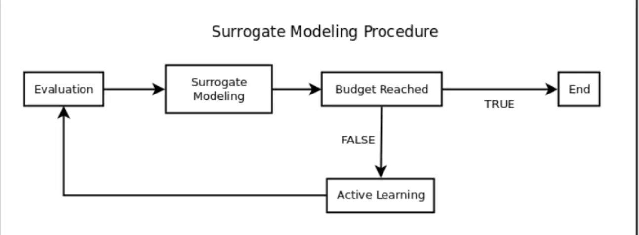
3.1 Structure of the surrogate
Here, we employ an iterative training procedure (see Figure1) to construct a different surrogate at each of several rounds until we approach a predefined budget of evaluations on the true ABM. At each round an additional parameter vectors is used in the iterative procedure. The budget 7Notwithstanding its precision, the surrogate remains an approximation of the original model. We suggest
the user, in any case, to identify positive calibrations and further study model’s behaviour therein and in their close neighbourhoods employing the original ABM.
8
Figure 1: Surrogate modelling algorithm.
is set in advance by the user according to a pre-determined, acceptable, computation cost of learning the surrogate. In each round, a surrogate is trained using all available parameter vectors, and their respective labels, which have been aggregated up to that round. Once the budget of evaluations is reached, the final surrogate is ready to be used for parameter space exploration.
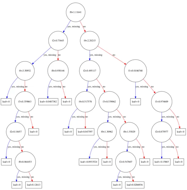
Here, we rely on XGBoost (Chen and Guestrin,2016) as our surrogate learning algorithm. This algorithm sequentially learns an ensemble of classification and regression trees (CART, see Breiman et al., 1984). Figure 2provides an example of CART tree. Given that the CART trees are represented as functions, the gradient resulting from the ensemble of CART trees can be minimized. Weights are assigned to each of the parameter vectors and “boosted” in the direction of the gradient that minimizes the total loss. Boosting magnifies the importance of difficult-to-learn samples. In each of the subsequent rounds, a new tree is learned over the boosted parameter vectors, incurring an increased penalty according to the boosted weights. Accordingly, trees are learned according to the weight from the previous round. The XGBoost algorithm builds CART trees that are increasingly specialized to handle the particular subset of samples that were difficult to learn up until the current round. A common way to characterize this learning procedure is to consider it as an ensemble of “weak” approximations, that together construct a strong approximation (see Freund, 1990; Freund et al., 1996; Chen and Guestrin,
2016, for more details see).
3.2 Surrogate performance evaluation
A trained surrogate can be used to efficiently explore the behaviour of the ABM over the entire parameter space. Relevant parameter combinations can then be selected for evaluation using the original ABM. Given the desire to avoid evaluating the computationally expensive true ABM, while also identifying positive calibrations, it is critical to maximize the performance of the surrogate to predict these calibrations. We recall that positive calibrations are points in the parameter space that fulfil the specific conditions, specified by an ABM modeller/user. Such conditions might include any test that compares simulated output with real data (e.g. distance between real and simulated moments, a non-parametric test on distribution equality,
Figure 2: An example classification and regression tree (CART) used for regression. Features are labelledf0, . . . , f4 and nodes specify cutoff thresholds that designate the path a new parameter vector takes from the top (root) node to the final (leaf) node, which denotes the predicted calibration value. In the process of “boosting” CART trees to produce an ensemble, each subsequent tree increasingly focuses on the higher weighted samples. This generally results in smaller “specialized” trees that stick on samples that were most difficult to classify.
mean squared prediction errors, etc.) and/or any specific feature the model might generate (e.g. fat tails in a specific distribution, growth rates of any variable above or below a given threshold, correlation patterns among a set of variables, etc.). In the two exercises presented in this paper (cf. Sections4 and 5below), both types of conditions are evaluated.
An effective surrogate should maximize the “True Positive Rate” (TPR). Given a set of parameter combinations, the TPR measures the number of positive calibrations predicted by a learned surrogate model against the actual number of positive calibrations possible in the parameter space. Automated hyper-parameter optimization procedures maximize the
perfor-mance of the machine learning surrogate according to a learning score or metric.9 Though our aim is to maximize the TPR of our surrogate, the scores used to train the surrogate depend on the particular form of the output condition. According to the two settings introduced above we distinguish between:
• Binary outcome. In this case the output of the calibration condition is discrete, such as Accept/Reject, and a measure of classification ability is needed. Specifically, we aim at maximizing theF1-score.10 TheF1-score is an harmonic mean betweenp, which indicates
the ratio between true positives and total positives and r, which represents the ratio of true positives to predicted ones:
F1= 2
p·r
p+r, (1)
The F1-score takes a value between 0 and 1. In terms of Type I and Type II errors, it
equates to:
F1 =
2·true positives
2·true positives + false positives + false negatives. (2) • Real-valued outcome. In this case, our aim is to minimize the mean-squared error
(MSE),
M SE=
PN
i=1(ˆyi−yi)2
N , (3)
where the surrogate predicts ˆyi overN evaluation points with a true labellingy. We notice
that this approach is in line, for instance, withRecchioni et al. (2015).
3.3 Parameter importance
The XGBoost algorithm employed in our surrogate modelling procedure allow us also to perform parameter sensitivity analysis at no costs. In particular, the machine learning algorithm provides an intuitive procedure of assessing the explained variance of the surrogate according to the relative number of times a parameter was “split-on” in the ensemble (for details see e.g.Archer and Kimes,2008;Louppe et al.,2013;Breiman,2001). As each tree is constructed according to an optimized splitting of the possible values for a specific parameter vector, and it is increasingly focusing on difficult-to-predict samples, splits dictate the relative importance of parameters in discriminating the output conditions of the ABM. Accordingly, the relative number of splits over a specific parameter provides a quantitative assessment of the sensitivity of the surrogate to the parameter and importance of that parameter to the user-specified conditions. As a consequence, this allows to rank model’s parameters on the basis of their importance in producing a behaviour of the model that satisfy whatever condition the user specifies. As this procedure is non-parametric, the resulting values should be interpreted as a rank-based statistic. The particular values associated to the number of splits only characterize the specific instantiation of the ensemble. Specifically, a different number of trees would result in changes to the split count
9
Several procedures exist for tuning machine learning hyper-parameters, see e.g. Feurer et al.(2015).
10
Note that there is “no free lunch” with regard to performance measures, so their choice depends on the problem setting (see e.g. Wolpert, 2002) For a detailed description of the F1-Score, see e.g. Van Rijsbergen
for each feature. The resulting counts provide insight into the relative performance for each parameter. As the number of trees approaches infinity, the number of splits will converge to the true ratio per feature by the law of large numbers.
3.4 Training procedure
The primary constraint we face is the limited number of parameter combinations that can be used for model evaluation (budget) without incurring in excessive computational costs. To address this issue, we propose abudgeted online active semi-supervised learning approach that iteratively builds a training set of parameter vectors on which the agent-based model is actually evaluated in order to provide labelled data points for the training of the surrogate. The aim of actively sampling the parameter space is to reduce the discrepancy between the regions that contain a manifold of interest and the function approximation produced by the surrogate model. This semi-supervised learning approach (see e.g. Zhu, 2005; Goldberg et al., 2011) minimizes the number of required evaluations, while improving the performance of the surrogate. Given that evaluated parametrizations are aggregated over several rounds and the stationary nature of the parameter space labels, we can use the log convergence results proved in Ross et al.
(2011) to provide a guideline on the number of parametrizations to evaluate in each round. In particular, we set the initial starting round to include at least one positive calibration and each of the subsequent rounds to log budget.
Our active learning approach relies on the assumption that positive calibrations represent a very small percentage of points in the parameter space. Leveraging on such an imbalance, our approach iteratively selects a random subset of positive predicted calibrations over a finite number of rounds. In order to maximize computing speed, the algorithm is initialized with a fixed subset of evaluated parameter combinations that are drawn according to a quasi-random Sobol sampling over the parameter space (Morokoff and Caflisch,1994).11 Further, the number of samples are drawn according to the ones required for “total variation” analysis presented in
Saltelli et al.(2010). These initial “training” points are then evaluated through the ABM, their labels recorded and finally used to initialize the first surrogate model. Once the surrogate is trained, new parameter combinations are sampled over the entire parameter space and labelled using the surrogate. A random subset of pointsxi are then selected from the predicted positive
calibrations of the surrogate and evaluated for their true labels yi using the ABM. Given the
log convergence rates presented in
These new points are then added to the training set to train a new surrogate in the next round. This “self-training” procedure exploits the imbalance in the data to incrementally in-crease true positives, while reducing false positives. Note that this simple self-training procedure may result in no new predicted positives. In this case, the algorithm selects new points accord-ing to their predicted binary label entropy, where the latter is defined as the entropy between the predicted positive and negative calibration label probabilities. This incremental procedure continues until the targeted training budget is achieved. The algorithm pseudo-code is presented in Figure 3.
11
Note that in high dimensional spaces, standard design of experiments are computationally costly and show little or no advantage over random sampling (Bergstra and Bengio,2012;Lee et al.,2015).
Set:
• Agent Based Model ABM∈RJ
• Sampling distributionν∈ RJ
• Calibration functionC(·)
• Learning algorithmA, with parameters Θ
• Evaluation budgetB
• Initial training set sizeN B • XT raining ∈
RN×J
• Calibration labelsYT raining ∈
NN binary outcome case (at least 1 positive calibration)
• Calibration labelsYT raining ∈
RN real-valued outcome case (at least 1 posi-tive calibration)
• Hyper-parameter optimization algorithm (HPO)
Initialize:
• Per-round sampling sizeSB • Per-round out-of-sample sizeKB While|Y|< B, repeat
1. Θ = HPO(A(Θ, XT raining, YT raining))
2. Draw out-of-sample pointsXOOS∈
RK×J ∼ν 3. SelectXsample ∈
RS×J fromXOOS 4. EvaluateXT raining =XT raining∪Xsample
5. EvaluateYsample={C(ABM(Xsample
i ))}i=1...S
6. EvaluateYT raining=YT raining∪Ysample
end while
Figure 3: Pseudo-code of our training algorithm. Note: Y indicates labels; X indicates param-eter vectors. HPO: hyper paramparam-eter optimization; OOS: out of sample
4
Surrogate modelling examples: The Brock and Hommes model
In their seminal contribution, Brock and Hommes (1998) develop an asset pricing model (re-ferred here as B&H), where an heterogeneous population of agents trade a generic assets ac-cording to different strategies (fundamentalist, chartists, etc.). In what follow, we first briefly introduce the model (cf. Section4.1). We then report the empirical setting (see Section4.2) and the results of our machine learning calibration and exploration exercise (cf. Section 4.3). We recall that the seed of the pseudo-random number generator is fixed and kept constant across runs of the model over different parameter vectors.4.1 The B&H asset pricing model
There is a population of N traders that can invest either in a risk free asset, which is perfectly elastically supplied at a gross returnR= (1 +r)>1, or in a risky one, which pays an uncertain dividend y and has a price denoted byp. Wealth dynamics is given by
Wt+1=RWt+ (pt+1+yt+1−Rpt)zt, (4)
wherept+1 andyt+1 are random variables andzt is the number of the shares of the risky asset
bought at time t.
Traders are heterogeneous in terms of their expectations about future prices and dividends and are assumed to be myopic mean-variance maximizers. However, as information about past prices and dividends is publicly available in the market, agents can apply conditional expected value Et, and variance Vt. The demand for sharezh,t of agents with expectations of type h is
computed solving: max zh,t Eh,t(Wt+1)− ν 2Vh,t(Wt+1) , (5)
which in turns implies
zh,t =Eh,t(pt+1+yt+1−Rpt)/(νσ2), (6)
whereν controls for agents’ risk aversion andσ indicates the conditional volatility, assumed to be equal across traders and constant over time. In case of zero supply of outside shares and different trader types, the market equilibrium equation can be written as:
Rpt=
X
nh,tEh,t(pt+1+yt+1), (7)
wherenh,t denotes the share that traders of typeh hold at timet. In presence of homogeneous
traders, perfect information and rational expectations, one can derive the no-arbitrage market equilibrium condition:
Rp∗t =Et(pt∗+1+yt+1), (8)
where the expectation is conditional on all histories of prices and dividends up to time t and where p∗ indicates the fundamental price. In case dividends are independent and identically distributed over time with constant mean, equation (8) has a unique solution where the fun-damental price is constant and equal to p∗ =E(yt)/(R−1). In what follows, we will express
prices as deviations from the fundamental price, i.e. xt=pt−p∗t.
At the beginning of each trading period t = {1,2, ..., T}, agents form expectations about future prices and dividends. Agents are heterogeneous in their forecasts. More specifically, investors believe that, in a heterogeneous world, prices may deviate from the fundamental value by some functionfh(·) depending upon past deviations from the fundamental price. Accordingly,
the beliefs aboutpt+1 and yt+1 of agents of type h evolve according to:
Eh,t(pt+1+yt+1) =Et(pt∗+1) +fh(xt−1, ..., xt−L). (9)
Many forecasting strategies specifying different trading behaviours and attitudes have been studied in the economic literature, (see e.g. Banerjee, 1992; Brock and Hommes, 1997; Lux and Marchesi, 2000; Chiarella et al., 2009). Brock and Hommes (1998) adopt a simple linear representation of beliefs:
fh,t =ghxt−1+bh, (10)
where gh is the trend component and bh the bias of trader type h. If bh 6= 0, the agent h
can be either a pure trend chaser if gh > 0 (strong trend chaser if g > R), or a contrarian if g <0 (strong contrarian if g < R). If gh 6= 0, the agent of type h is purely biased (upward or
downward biased if bh > 0 or bh < 0). In the special case when both gh and bh are equal to
zero, the agent is a “fundamentalists”, i.e. she believes that prices return to their fundamental value. Agents can also be fully rational, withfrational,t =xt+1. In such a case, they have perfect
foresight but, they must pay a cost C.12
In our application, we use a simple model with only two types of agents, whose behaviours vary according to the choice of trend components, biases and perfect forecasting costs. Com-bining equations (7), (9) and (10), one can derive the following equilibrium condition:
Rxt=n1,tf1,t+n2,tf2,t, (11)
which allows to compute the price of the risky asset (in deviation from the fundamental) at timet.
Traders switch among different strategies according to the their evolving profitability. More specifically, each strategyh is associated with a fitness measure of the form:
Uh,t = (pt+yt−Rpt−1)zh,t−Ch+ωUh,t−1 (12)
where ω∈[0,1] is a weight attributed to past profits. At the beginning of each period, agents reassess the profitability of their trading strategy with respect to the others. The probability that an agent choose strategy his given by:
nh,t =
exp(βUh,t)
P
hexp(βUh,t)
, (13)
12In our experiments we allow for the possibility that a positive cost might be by paid also by non-rational
traders. This mirrors the fact that some trader might want to buy additional information, which they might not be able to use (due e.g. to computational mistakes).
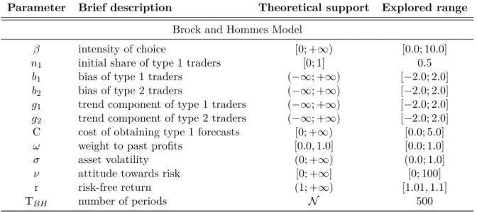
Table 1: Parameters and explored ranges in the Brock and Hommes model.
Parameter Brief description Theoretical support Explored range
Brock and Hommes Model
β intensity of choice [0; +∞) [0.0; 10.0]
n1 initial share of type 1 traders [0; 1] 0.5
b1 bias of type 1 traders (−∞; +∞) [−2.0; 2.0]
b2 bias of type 2 traders (−∞; +∞) [−2.0; 2.0]
g1 trend component of type 1 traders (−∞; +∞) [−2.0; 2.0]
g2 trend component of type 2 traders (−∞; +∞) [−2.0; 2.0] C cost of obtaining type 1 forecasts [0; +∞) [0.0; 5.0]
ω weight to past profits [0.0,1.0] [0.0; 1.0]
σ asset volatility (0; +∞) (0.0; 1.0]
ν attitude towards risk [0; +∞] [0; 100] r risk-free return (1; +∞) [1.01,1.1]
TBH number of periods N 500
where the parameter β ∈ [0,+∞) captures traders’ intensity of choice. According to equation
13, successful strategies gain an increasing number of followers. In addition, the algorithm introduces a certain amount of randomness, as less profitable strategies may still be chosen by traders. In this way, the model captures imperfect information and agents’ bounded rationality. Moreover, the system can never be stacked in an equilibrium where all traders adopt the same strategy.
4.2 Experimental design and empirical setting
Despite the model is relatively simple, different contributions have tried to match the statistical properties of its output with those observed in real financial markets (Boswijk et al., 2007;
Recchioni et al.,2015;Lamperti,2016;Kukacka and Barunik,2016). This makes the model an ideal test case for our surrogate: it is relatively cheap in terms of computational needs, it offers a reasonably large parameter space and it has been extensively studied in the literature.
There are 12 free parameters (Table 1) whose values are to be determined trough cali-bration.13 The ranges for parameters’ values have been identified relying on both economic reasoning and previous experiments on the model. However, their selection is ultimately a user specific decision. Our procedure allow to deal with large parameter spaces, thus minimizing the constraints face by modellers. In what follows, we refer to the parameter space spanned by the intervals specified in the last column of Table 1. Naturally, it can be further expanded or reduced according to the user’s needs and the available budget.
Let us now consider the conditions identifying positive calibrations. As already discussed above, any feature of model’s output can be employed to express such conditions. According to Section 3 two types of calibration criteria are considered, giving respectively binary and real-valued outcomes. In the binary outcome case, we employ a two samples Kolmogorov-Smirnov (KS) test between the distribution of logarithmic returns obtained from the numerical simulation 13We underline that the dimension of the parameter space is in line or even larger that in recent studies on
of the model and the one obtained from real stock market data.14 More specifically, we rely on daily adjusted closing prices for the S&P 500 going from December 09, 2013 to December 07, 2015, for a total of 502 observations, and we compute the following test statistic:15
DRW ,S = sup r
|FRW(r)−FS(r)|, (14)
wherer indicate logarithmic returns andFRW and FS are the empirical distribution functions
of the real world (RW) and simulated (S) samples respectively. Then, in a real-valued outcome setting, we use the p-value of the KS test, P(D > DRW,S), as an expression of model’s fit
with the data. In particular, the higher the p-value of the test, the more difficult to reject the null and the larger the fit with the data. We also consider an equivalent condition for the binary outcome: predicted labels above 5% indicate positive calibrations. The choice is made on purpose: using equivalent conditions allows to compare the binary and real-valued outcome in terms of precision (ability to identify true calibrations) and computational time (in the real-valued scenario there is more information to be processed.)
We train the surrogate 100 times over 10 different budgets of 250, 500, 750, 1000, 1250, 1500, 1750, 2000, 2250, 2500 labelled parameter combinations and evaluate it on 100000 unlabelled points. Having a large number of out-of-sample, unlabelled, possibly well-spread points is fundamental to evaluate the performance of the meta-model. We use a larger evaluation set than any other meta-modelling contribution we are aware of (see, for instance,Salle and Yildizoglu,
2014;Dosi et al.,2017c;Bargigli et al.,2016).
4.3 Results
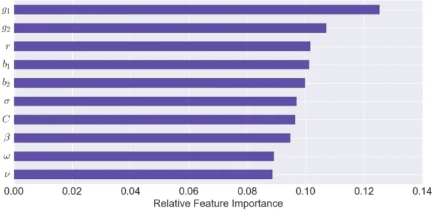
In Figure 4, we show the parameter importance results for the Brock and Hommes (B&H) model. We find that the most relevant parameters to fit the empirical distribution of returns observed in the SP500 are those characterizing traders’ attitude towards the trend (g1 and g2)
and, secondly, their bias (b1 andb2). This result is in line with recent findings byRecchioni et al.
(2015) and Lamperti (2016) obtained using the same model. Moreover, the intensity of choice parameter (β, cf. Section4), which is of crucial importance in the original model developed by
Brock and Hommes (1998), does not appear to be particularly relevant in determining the fit of the model with the data if compared to other behavioural parameters (at least within the range expressed by Table 1, ).16 Also traders’ risk attitude (α) and the weight associated to past profits (ω) are relatively unimportant to shape the empirical performance of the model.
Let us now consider the behaviour of the surrogate. As outlined in Section 3.2, we run a series of exercises where the surrogate is employed to explore the behaviour of the model over the parameter space and filter out positive calibrations matching the distribution of real stock-market returns. Figure 5 collects the results and show the performance of the surrogate in the two proposed settings (binary and real-valued outcome). Within the binary outcome
14
Letpt andpt−1 be the prices of an asset at two subsequent time steps. The logarithmic return fromt−1 to
tis given byrt= log(pt/pt−1)'(pt−pt−1)/pt−1. 15
The data have been obtained from Yahoo Finance: https://finance.yahoo.com/quote/%5EGSPC/history. The test is passed if the null hypothesis “equality of the distributions” is not rejected at 5% confidence level.
16See also Boswijk et al. (2007) where the authors estimate the B&H model on the SP500 and, in many
Figure 4: Importance of each parameter (feature) in shaping behaviour of the Brock and Hommes model according to the specified conditions (i.e. equality between distributions of simulated and real returns). As noted in Section 3.3, this chart demonstrates the relative rank-based importance for each parameter.
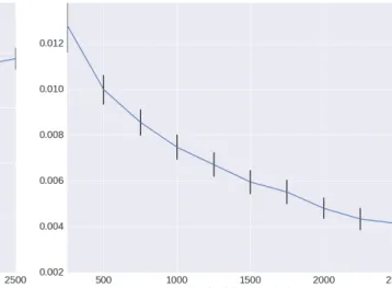
exercise, the F1-score is steadily increasing with the size of the training sample and it reaches
a peaking value of around 0.80 when 2500 points are employed (cf. Figure5a). In other words, the average between the share of true positive calibrations and the share of positive calibrations the surrogate correctly predicts is 0.8. Taken into consideration the upper bound of 1 and various practical applications (e.g. Petrovic et al.,2011;Cire¸san et al., 2013), we consider the former result satisfying. However, such a classification performance should be evaluated in view of the surrogate’s searching ability, which is reported in Figure 5c and indicates the share of total positive calibration that the surrogate is able to find. Specifically, we find that around 75% of the positive calibrations present in the large set of out-of-sample points are found.
Obviously, the surrogate’s performance worsens as the training sample size is reduced. How-ever, once we move to the real-valued setting, where the surrogate is learnt using a continuous variable (containing more information about model’s behaviour), its performance is remarkably higher. Indeed, even when the sample size of the training points is particularly low (500), the True Positive Ratio (TPR) is steadily around 70%, and it reaches almost 95% (on average) when 2500 parameter vectors are employed (see Figure 5d).
Timing results are reported according to the average seconds required for a single compute core to complete the specific task 100 times. The increase in performance from classification (see Figure 5e) to regression (see Figure 5f) requires roughly 3X the modelling time and a nearly equivalent prediction time. Given this negligible prediction time, our approach facilitates a nearly costless exploration of the parameter space, delivering good results in terms ofF1-score,
TPR and MSE. The time savings in comparison to running the original ABM are substan-tial. In this exercise over a set of 10000 out-of-sample points, the surrogate is 500X faster on average in prediction. Note also that the learned surrogate is reusable on any number of out-of-sample parameter combinations, without the need for additional training. Further, we remark
(a) Binary-outcome: F1 Score (b) Real-valued outcome: Mean Squared Error
(c) Binary-outcome: True Positive Rate (d) Real-valued outcome: True Positive Rate
(e) Binary-outcome: Computation Time (f) Real-valued outcome: Computation Time
Figure 5: Brock and Hommes surrogate modelling performance averaged over a pool of 10000 parametrizations. Black vertical lines indicate 95% confidence intervals on 100 repeated and independent experiments.
that computational gains are expected to be larger as more complex and expensive-to-simulate models are used. The next section goes in this direction.
5
Surrogate modelling examples: the Islands model
In the “Island” growth model (Fagiolo and Dosi,2003), a population of heterogeneous firms lo-cally interact discovering and diffusing new technologies, which ultimately lead to the emergence (or not) of endogenous growth. After having presented the model (Section 5.1), we describe the empirical setting (see Section 5.2) and the results of the machine learning calibration and exploration exercises (cf. Section 5.3). We recall that the seed of the pseudo-random number generator is fixed and kept constant across runs of the model over different parameter vectors.
5.1 The Island growth model
A fixed population of heterogeneous firms (I = 1,2, ..., N) explore an unknown technological space (“the sea”), punctuated by islands (indexed byj= 1,2, ...) representing new technologies. The technological space is represented by a 2-dimensional, infinite, regular lattice endowed with the Manhattan metrics d1. The probability that each node (x, y) is an island is equal to
p(x, y) =π. There is only one homogeneous good, which can be “mined” from any island. Each island is characterized by a productivity coefficientsj =s(x, y)>0. The production of agenti
on islandj having coordinates (xj, yj) is equal to:
Qi,t =s(xj, yj)[mt(xj, Yj)]α−1, (15)
where α≥1 and mt(xj, yj) indicates the total number of miners working onj at time t. The
GDP of the economy is simply obtained summing up the production of each island.
Each agent can choose to be aminer and produce an homogeneous final good in her current island, to become anexplorerand search for new islands (i.e. technologies), or to be animitator
and seal towards a known island. In each time step, miners can decide to become explorer with probability > 0. In that case, the agent leaves the island and “sails” around until another (possibly still unknown) island is discovered. During the search, explorers are not able to extract any output and randomly move in the lattice. When a new island (technology) is discover, its productivity is given by:
sjnew = (1 +W){[|xjnew|+|yjnew|] +ϕQi+ω} (16) whereW is a Poisson distributed random variable with meanλ >0,ωis a uniformly distributed random variable with zero mean and unitary variance, ϕ is a constant between zero and one and, finally,Qi is the output memory of agenti. Therefore, the initial productivity of a newly
discovered island depends on four factors (see Dosi, 1988): (i) its distance from the origin; (ii) cumulative learning effects (φ); (iii) a random variable W capturing radical innovations (i.e. changes in technological paradigms); (iv) a stochastic i.i.d. zero-mean noise controlling for high-probability low-jumps (i.e. incremental innovations).
Table 2: Parameters and explored ranges in the Island model.
Parameter Brief description Theoretical support Explored range
Islands Model
ρ degree of locality in the diffusion of knowledge [0,+∞) [0; 10]
λ mean of Poisson r.v. - jumps in technology [0; +∞) 1
α productivity of labour in extraction [0,+∞) [0.8; 2]
ϕ cumulative learning effect [0,1] [0.0; 1.0]
π probability of finding a new island [0.0,1.0] [0.0; 1.0]
willingness to explore [0,1] [0.0; 1.0]
m0 initial number of agents in each island [2,+∞) 50
TIS number of periods N 1000
informational spill-overs stemming from more productive islands located in their technological neighbourhoods. More specifically, agents mining on any colonized island deliver a signal, which is instantaneously spread in the system. Other agents in the lattice receive the signal with probability:
wt(xj, yj;x, y) =
mt(xj, yj) mt
exp{−ρ[|x−xj|+|y−yj|]}, (17)
which depends on the magnitude of technology gap as well as on the physical distance between two islands (ρ > 0). Agent i chooses the strongest signal and become an imitator sealing to island according to the shortest possible path. Once the imitated island is reached, the imitator will start mining again.
The model shows that the very possibility of notionally unlimited (albeit unpredictable) technological opportunities is a necessary condition for the emergence of endogenous exponen-tial growth. Indeed, self-sustained growth is achieved whenever technological opportunities (captured by both the density of islands π and the likelihood of radical innovations λ), path-dependency (i.e. the fraction of idiosyncratic knowledge, ϕ, agents carry over to newly discov-ered technologies), and spreading intensity in the information diffusion process (ρ), are beyond some minimum thresholds (Fagiolo and Dosi,2003). Moreover, the system endogenously gener-ate exponential growth if the trade-off between exploration and exploitation is solved, i.e. if the ecology of agents find the right balance between searching for new technologies and mastering the available ones.
5.2 Experimental design and empirical setting
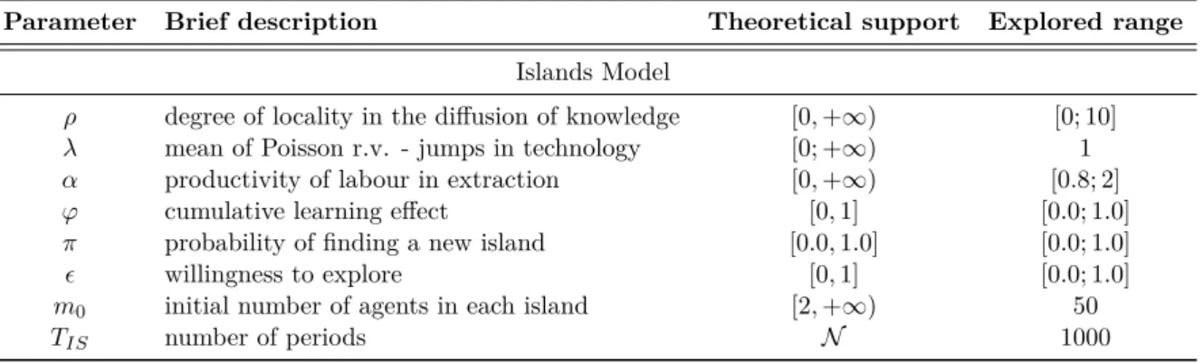
The Island model employs eight input parameters to generate a wide array of growth dynamics. We report the parameters, their theoretical support and the explored range in Table 2. We kept the number of firms fixed (and equal to 50) to study what happens to the same economic system, when the parameters linked to behavioural rules are changed.17
Similarly to section4.2, we characterize a binary outcome and a real-valued outcome setting. In the first case, the surrogate is learnt using a binary target variabley taking value 1 if a user-defined specific set of conditions is satisfied and zero otherwise. More specifically, we define 17Note that the Island model does not exhibit scale effects: the results generated by the model does not depend
two conditions characterizing the GDP time series generated by the model. The first condition requires the model to generate self-sustained sustained pattern of output growth. Given the long-run average growth rate of the economy (AGR):
AGR= log(GDPT)−log(GDP1)
T−1 , (18)
sustained growth emerges ifAGR >2%.
The second condition aims at capturing the presence of fat tails in the output growth-rate distributions. This empirical regularities, which suggest that deep downturns coexist with mild fluctuations has been found in both OECD (Fagiolo et al., 2008) and developing countries (Castaldi and Dosi,2009;Lamperti and Mattei,2016). More specifically, we fit a symmetric ex-ponential power distribution (seeSubbotin,1923;Bottazzi and Secchi,2006) , whose functional form reads: f(x) = 1 2ab1bΓ(1 + 1 b) e−1b| x−µ a | b (19) whereacontrols for the standard deviation,bfor the shape of the distribution andµrepresents the mean. As bgets smaller, the tails become fatter. In particular, whenb= 2 the distribution reduces to a Gaussian one, while for b = 1 the density is Laplacian. We say that the output growth-rate distribution exhibits fat tails ifb≤1. Note that there is a hierarchy in the conditions we have just defined: only those parametrizations satisfying the first one (AGR > 2%) are retained as candidates for positive calibrations and further investigated with respect to the second condition. In the real-valued outcome case, instead, we just focus on shape of growth rates distribution. In particular, we our target variable is the estimatedbof the symmetric power exponential distribution and a positive calibration is found ifb >1.18 Again, the choice of the condition to be satisfied ensures (partial, in this case) consistency between the two settings.
We train the surrogate as we did with the B&H model, but given the higher computational complexity of the Island model, we reduce the number of unlabelled points to 10000.19
5.3 Results
As for the Brock and Hommes model, we start our analysis reporting the relative importance for all the parameters characterizing the Island model (figure 6). We find that all the parameters of the model linked to production, innovation and imitation appear to be relevant for the emergence of sustained economic growth.
The surrogate’s performances is presented in Figure 7, where the first column of the plots refers to the binary outcome setting, while the second one to the real-valued one. The F1
-score displays relatively high values even for low training sample sizes (250 and 500) pointing to a good classification performance of the surrogate (see Figure 7a). However, it quickly saturates, reaching a plateau around 0.8. Conversely, in the real-valued setting, the surrogate’s performance keeps increasing with the training sample size, and it displays remarkably low
18
In the real-valued outcome setting our exercise is comparable to those performed inDosi et al.(2017c), where the same distribution and parameters are used in a model of industrial dynamics.
19
This choice is motivated by the fact that we need to run the model on the out-of-sample points in order to evaluate the surrogate.
Figure 6: Importance of each parameter (feature) in shaping behaviour of the Islands model according to the specified conditions (sustained growth and fat tails). As noted in Section 3.3, this chart demonstrates the relative rank-based importance for each parameter.
Surrogate Algorithm True Negatives False Positives False Negatives True Positives Precision
Logit 62 22 61 355 94.17%
XGBoost 178 17 0 305 94.72%
XGBoost (scaled) 193 2 0 305 99.35%
Table 3: Surrogate modelling performance using the learning procedure presented in this paper.
values of MSE when more than 1000 points are employed (cf. Figure7b).
In both settings, the searching ability of the surrogate behaves in a similar way: the TRP steadily increases with the training sample size (cf. Figures 7c and 7d). In absolute terms, the real-valued setting delivers much better results than the binary one, as for the Brock and Hommes model (section 4.3). In particular, the largest true positive ratio reaches 0.9 for the real-valued case and 0.8 for the binary one. Therefore, by training the surrogate on 2500 points we are able to (i) find 90% of true positive calibrations (Figure7d) and predict the thickness of the associated distribution of growth rates incurring in a mean squared error of less than 0.08 (Figure7b) using a continuous target variable and, (ii) find 80% of the true positives (panel7c) and correctly classifying around the 80% of them (panel 7a) using a binary target variable.
Given the satisfactory explanatory performance of the surrogate, do we also achieve consid-erable improvements in the computational time required to perform such exploration exercises? Figures 7e and 7f provides a positive answer. Indeed, the surrogate is 3750 times faster than the fully-fledge Island agent-based model. Moreover, the increase in speed is considerably larger than in the Brock and Hommes model. This confirms our intuition on the increasing usefulness of our surrogate modeling approach when the computational cost of the ABM under study is higher. Such a result is a desirable property for real applications, where the complexity of the underlying ABM could even prevent the exploration of the parameter space.
(a) Binary-outcome: F1 Score (b) Real-valued outcome: Mean Squared Error
(c) Binary-outcome: True Positive Rate (d) Real-valued outcome: True Positive Rate
(e) Binary-outcome: Computation Time (f) Real-valued outcome: Computation Time
Figure 7: Islands surrogate modelling performance versus budget size averaged over a pool of 10000 parametrizations. Black vertical lines indicate 95% confidence intervals on 100 repeated and independent experiments.
5.4 Robustness analysis
We now assess the robustness of our training procedure with respect to different surrogate models. More specifically, we compare the XGBoost surrogate employed in the previous analysis with the simpler and more widely used Logit one. Our comparison exercise is performed in a fully stochastic version of the Island agent-based model, where an additional Monte Carlo (MC) is carried out on the seed parameter governing the stochastic terms of the model. As a sneak preview, we can anticipate that our procedure is pretty robust to different surrogate crus.
We focus on a binary outcome setting (the one delivering worse performances) and we employ the milder condition that the average growth rate must be positive and sustained, i.e.
AGR > 0.5%. In this way, the results can be compared to those obtained in the original exercise in Fagiolo and Dosi (2003). We set a budget of 500 evaluations of the “true” Islands ABM and run a Monte Carlo exercise of size 100 per parameter combination to generate an MC average of the GDP growth rate that serves as our output variable. Note that this exercise is more complete that the one performed in the previous sections: here, we develop a surrogate model that learns the relationship between parameters and the MC average over their ABM evaluations. Note that this requires many more evaluations of the parameter combination in the true ABM to converge to the statistic required for the label. In our proposed procedure, an MC average growth rate below 0.5% is labelled “false”, while AGR above 0.5% are labeled “true”. The aim is to learn a surrogate model that accurately classifies parameter combinations as positive or negative calibrations.
We demonstrate the performance of our active learning approach using two different surro-gates: the XGBoost and the faster, less precise, Logit. The former, employed in the analyses carried out in the previous sections, benefits from increased accuracy in exchange for greater computational costs. The latter is a standard statistical model employed regularly for this type of regression analysis. The performance of these alternative surrogates will be evaluated according to the F1-score while training the surrogate, with the final objective of maximizing the precision of the resulting models, i.e. the number of true evaluations which are accurately predicted as positive before they are evaluated. This is a key point to this exercise because real-world use of the proposed approach does not allow us to evaluate all the points in our sample space. Real-world evaluation only provides labels for points that are predicted positive and the resulting performance can only be measured with regard to the true and false positives, with a preference to maximize the former.
The exercise is performed using the Python BOASM package.20 The algorithm mirror ex-actly the one described in Section3. The exercise begins by sampling 1000000 points at random from the Islands parameter space. Given the fixed budget of 500 evaluations of the true ABM, for both the XGBoost and Logit, the first surrogate is provided with 35 labelled parameters se-lected at random from the 1000000 points, according to the total-variation sampling procedure inSaltelli et al.(2010). Then, over several rounds, a surrogate will be fit to the labelled param-eters and used to predict a labelling over the 1000000 points. The predicted labels will then be employed by the proposed procedure to select points that will be added at each round to the set of labelled points. A new surrogate is learned in the subsequent round and the procedure