Received April 29th, 2015, Revised January 7th, 2016, Accepted for publication February 19th, 2016. Copyright ©2016 Published by ITB Journal Publisher, ISSN: 2337-5779, DOI: 10.5614/j.eng.technol.sci.2016.48.1.6
Probability-based Evaluation of Vehicular Bridge Load
using Weigh-In-Motion Data
Widi Nugraha1,2 & Indra Djati Sidi3
1
Institute of Road Engineering, Ministry of Public Works and Housing, Republic of Indonesia, Jalan A.H. Nasution 264, Bandung 40294, Indonesia
2
Master Program Study of Civil Engineering, Faculty of Civil and Environmental Engineering, Institut Teknologi Bandung, Jalan Ganesha 10, Bandung 40132, Indonesia
3
Structural Engineering Research Group, Faculty of Civil and Environmental Engineering, Institut Teknologi Bandung, Jalan Ganesha 10, Bandung 40132, Indonesia
Email: [email protected]
Abstract. The Load and Resistance Factored Design (LRFD) method has been implemented for designing bridges in Indonesia for more than 25 years. LRFD treats load and strength variables as random variables with specific safety factors for different types of load and strength variables. The nominal loads, load factors, reduction factors, and other criteria from the bridge design code can be determined to meet the reliability criteria. Statistical data from weigh-in-motion (WIM) vehicular load measurements that were taken on North Java Highway Cikampek–Pamanukan, West Java (2011), were used in this study as statistical load variables. A 25 m simple span bridge with reinforced concrete T-girders was used as the model for structural analysis due to the WIM measured and nominal vehicular load based on the Indonesian bridge loading code RSNI T-02-2005, with the applied bending moment of the girders as the output. The distribution fitting result of the applied bending moment due to the WIM measured vehicular loads was lognormal. The maximum bending moment due to the nominal vehicular load from RSNI T-02-2005 is 842.45 kN-m and has a probability of exceedance of 5x10⁻⁵. It can be concluded from this study that the bridge designed using the standard loading from RSNI T-02-2005 was safe, since it has a reliability index (β) of 4.68, higher than the target reliability, ranging from 3.50 or 3.72.
Keywords: bridge; LRFD; probability; standard; vehicular load; weigh-in-motion.
1
Introduction
The Load and Resistance Factored Design (LRFD) method has been implemented for the designing of bridges in Indonesia for more than 25 years. LRFD treats load and strength variables as random variables with specific safety factors for different types of load and strength variables. The nominal loads, load factors, reduction factors and other criteria from the bridge design code can be determined to meet the reliability criteria. Conducting a reliability
analysis using Indonesian-based statistical data on loads and resistances is important for determining the nominal loads, load factors, reduction factors and any other criteria from the Indonesian LRFD bridge design code. LRFD bridge design codes must be evaluated periodically using actual statistical data on loads and resistances[1]. Therefore, the Indonesian bridge loading code RSNI T-02-2005 [2] also needs to be evaluated for calibration. The evaluation procedure has to make sure the target reliability conforms with the actual conditions. If the evaluation result denotes that the target reliability is not reached, the provisions in the LRFD code must be calibrated in order to reach the target reliability[3].
In this study, a reliability analysis was conducted to determine the reliability index (β) of a bridge structure that was designed using the vehicular nominal load provisions from the Indonesian bridge loading code RSNI T-02-2005 [2] when subjected to statistical load data of weigh-in-motion (WIM) vehicular load measurements that were taken on the Cikampek–Pamanukan highway (North Java Highway), Province of West Java, by the Institute of Road Engineering, Ministry of Public Works [4] in 2011. The WIM vehicular loads were measured from 29 October 2011 to 1 November 2011 for 3 x 24 hours in both directions of the highway. A simple span bridge of 25 m length with reinforced concrete T-girders was used as the model for the structural analysis due to the WIM measured vehicular loads and nominal vehicular load provision based on RSNI T-02-2005 [2]. The maximum bending moment of the girders as the output of the structural analysis due to WIM measured vehicular loads was collected and then analyzed statistically to determine the most fitted distribution using a goodness of fit (GOF) test [5] before it was used in the reliability analysis to calculate the reliability index (β). From the reliability analysis results, we evaluated the reliability index (β) result and compared it to the target reliability
of the AASHTO LRFD Bridge Design Specifications (3.50) [6] and the target reliability for new designed bridges with high priority of importance (3.75), as recommended by Nowak [7]. Then, the vehicular nominal load provisions in RSNI T-02-2005 [2] were calibrated to reach the target reliability (β) within the scope of this work.
2
Methodology
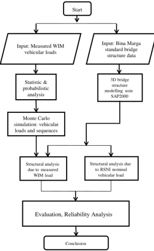
This research was organized according to the research methodology flowchart as shown in Figure 1. The primary data used in this research were statistical load data from WIM vehicular load measurements taken at the Cikampek– Pamanukan highway [4] and bridge structural data from Bina Marga standard reinforced concrete T-girders of a 25 m simple span bridge[8]. First, the vehicular load measurement data were processed statistically to calculate maximum value, minimum value, average value, standard deviation and
coefficient of variation (c.o.v). Then the Kolmogorov-Smirnov GOF test was used to determine the most fitted continuous distribution for these data. The distribution data of the axle loads for every vehicle class were then used as the basis for a Monte Carlo simulation [9] to determine the vehicular sample load.
Figure 1 Research methodology flowchart.
A Monte Carlo simulation was also used to simulate the vehicle class sequence combinations in the traffic lanes. This simulation was based on discrete distribution data of vehicle class composition during the WIM measurements. The random sequence of vehicle classes resulted from the Monte Carlo simulation was then cut into vehicle class sequence combinations on the bridge with the bridge length as the constraint. The vehicle class sequence combinations and vehicular class sample load were used for the WIM measured static loading model in the structural analysis. The vehicle sequences from the simulation were verified with the WIM data sequences. The bridge model was
Structural analysis due to RSNInominal
vehicular load
Evaluation, Reliability Analysis
Monte Carlo simulation: vehicular loadsand sequences
Structural analysis due to measured WIM load Statistic& probabilistic analysis Input: Measured WIM
vehicular loads
Start
Conclusion
Input: Bina Marga standard bridge structure data 3D bridge structure modellingusin SAP2000
also subjected to the vehicular nominal load provision based on Indonesian bridge loading code RSNI T-02-2005 [2].
The girders’ maximum bending moment due to the vehicular nominal load from RSNI T-02-2005 [2] was then evaluated by calculating its probability of exceedance in the distribution of the girder maximum bending moment due to the measured WIM load. Next, the reliability index of the bridge structure, designed based on the nominal vehicular load according to RSNI T-02-2005 [2], was calculated using the reliability analysis. From the reliability index result, we calculated the calibrated equivalent nominal vehicular load for a certain target reliability. According to the AASHTO LRFD Bridge Design Code [6], the target reliability is 3.50 for reinforced concrete and steel concrete. Since RSNI T-02-2005 [2] provisions are also based on the AASHTO LRFD Bridge Design Code [6], the target reliability must almost be the same. As an alternative, a target reliability value of 3.75 for new designed bridges with high priority of importance was used, as recommended by Nowak [7]. The conclusion is a technical recommendation, within the scope of this work, to calibrate the provisions of the vehicular nominal load in RSNI T-02-2005 [2] using the measured WIM vehicular load for certain target reliability (β) values.
3
Weigh-in-motion Statistical Data Processing
Weigh-in-motion Statistical Data
3.1
The weigh-in-motion (WIM) vehicular loads were measured on the Cikampek– Pamanukan highway (North Java Highway), Province of West Java by the
Table 1 EURO13 vehicle classifications. Vehicle
Class Classification
Axle Configuration
1 Car, Light Van MP 1.1
Light Good Vehicles T 1.2 & B. 1.2
2 Rigid 2-Axle Truck T 1.2
3 Rigid 3-Axle Truck T 1.22 4 Rigid 4-Axle Truck T 12. 22 5 Rigid 2-Axle Truck & Trailer T 1.2 + 22 6 Rigid 3-Axle Truck & Trailer T 1.22 + 22 7 2-Axle Tractor & 1-Axle Trailer T 12 - 2 8 2-Axle Tractor & 2-Axle Trailer T 1.22 - 22 9 2-Axle Tractor & 3-Axle Trailer T 1.22 - 222 10 3-Axle Tractor & 1-Axle Trailer T 1.22-2
3-Axle Tractor & 2-Axle Trailer T 1.22-22 11 3-Axle Tractor & 3-Axle Trailer T 1.22-222
Institute of Road Engineering, Ministry of Public Works [4] in 2011. The WIM vehicular loads were measured from 29 October 2011 to 1 November 2011 for 3 x 24 hours in both directions of the highway, i.e. in the Cirebon to Jakarta direction and in the Jakarta to Cirebon direction. The WIM measured vehicular load data as number of vehicles plotted versus vehicle class can be seen in Figure 2. The vehicle classification used by data logger (Marksman 660 – WIM System) in this measurement was the EURO13 classification, which classifies vehicles into 12 different classes [10], as shown in Table 1.
Figure 2 Number of vehicles versus vehicle class based on WIM measurements.
As can be seen in Figure 2, vehicle class 1 (described as car, light van, light good vehicles, etc. in EURO13) was measured as the vehicle class with the highest frequency, i.e. 35218 vehicles or 48.68% from the total of WIM measured vehicles.
Table 2 WIM measured vehicular load statistical data properties. Statistic Value Percentile Value (kgf)
Sample Size 72353 Min 412.31
Range 36573 5% 534.78
Mean 3488.2 10% 598.06
Variance 1.58E+07 25% (Q1) 791.97
Standard Deviation 3975 0% (Median) 2149.3 Coefficient of Variation 1.1396 75% (Q3) 4691.6
90% 11441
95% 36986
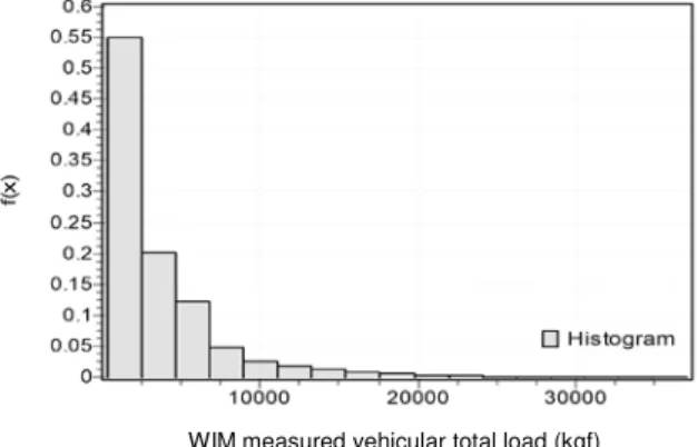
The statistical data properties and histogram of the measured vehicular load data respectively can be seen in Table 2 and Figure 3. Light vehicles with a low total weight had the highest probability density. This can be justified by the frequency number of the light vehicles class based on the WIM measurements having a higher frequency number than any other class.
Figure 3 Histogram of WIM measured vehicular load.
Distribution Fitting
3.2
Based on the classified WIM measured vehicular load data according to the EURO13 provision [10], the axle load data were treated as a random variable and the axle spacing was treated as a certain variable. Axle spacing for each vehicle class was taken from the minimal axle spacing provision from EURO13 to give the maximum load effect on the bridge structure. To determine the most fitted distribution of the WIM measured vehicular load data, the Kolmogorov-Smirnov goodness of fit (GOF) test was used [5]. In this test, the data distribution for each axle load class is determined. For example, Figure 4 below shows the probability density function (PDF) curves for the most fitted distribution for the WIM measured load of every front axle class (for 12 vehicle classes from EURO13, except vehicle class 7 which was not detected in the WIM measurements used). The PDF data for every axle load class were used to simulate the vehicular axle load sample using a Monte Carlo simulation [9], which was then used as the input load for the bridge structure model to be analyzed. In Figure 4 each vehicle class is represented by a variable designation consisting of four letters and numbers. The first letter (K) and the digit following the first letter represent the vehicle class. The second letter (S) and the digit following the second letter represent the axle number. For example, “K2S1” represents “axle number 1 of vehicle class number 2”.
(a) K1S1 (b) K2S1
(c) K3S1 (d) K4S1
(e) K5S1 (f) K6S1
Figure 4 PDF curve of WIM measured front axle load for each vehicle class.
Gamma (3P) PDF α =1.52 β =134.13 γ = 204.63 Lognormal (3P) PDF σ =0.46 μ =6.81 γ = 158.1 Lognormal (3P) PDF σ =0.163 μ =8.28 γ = -2054.9 Normal PDF σ =776.88 μ =2131.4 Lognormal (3P) PDF σ =0.286 μ =7.81 γ = -849.55 Normal PDF σ =478.73 μ =1787.8
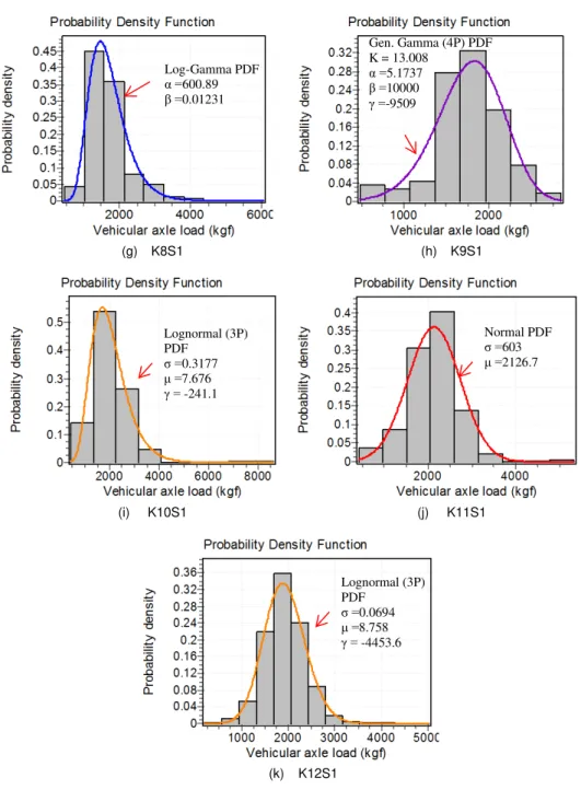
(g) K8S1 (h) K9S1
(i) K10S1 (j) K11S1
(k) K12S1
Figure 4 Continued. PDF curve of WIM measured front axle load for every
vehicle class. Log-Gamma PDF α =600.89 β =0.01231 Gen. Gamma (4P) PDF K = 13.008 α =5.1737 β =10000 γ =-9509 Lognormal (3P) PDF σ =0.3177 μ =7.676 γ = -241.1 Normal PDF σ =603 μ =2126.7 Lognormal (3P) PDF σ =0.0694 μ =8.758 γ = -4453.6
Vehicle Sequence Combinations
3.3
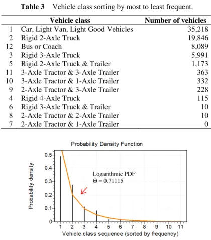
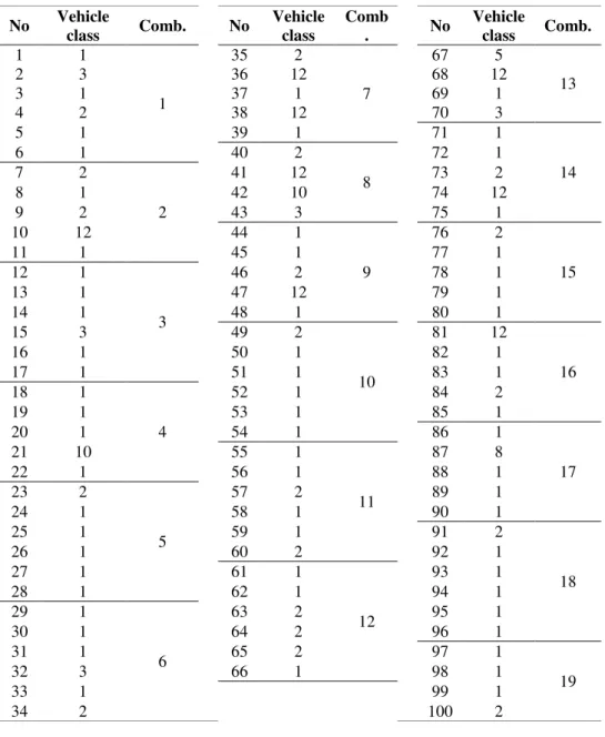
To determine the vehicle sequence combinations, first, the frequency data of each vehicle class was sorted from the highest to the lowest frequency number, as shown in Table 3. Then, the discrete distribution of the vehicle class frequencies was determined with the GOF test, as shown in Figure 5. Based on the distribution of vehicle class frequencies, the vehicle sequence combinations were simulated by withdrawing certain vehicle class samples using a Monte Carlo simulation, for which 100 samples were used in this study. Within the constraints of a 25 m bridge span length, the EURO13 vehicle axle spacing and length provision, and the assumption of a spacing between one vehicle to the next being 2 m representing traffic jam conditions, the vehicle sequence combinations were determined, as shown in Table 4.
Table 3 Vehicle class sorting by most to least frequent. Vehicle class Number of vehicles 1 Car, Light Van, Light Good Vehicles 35,218
2 Rigid 2-Axle Truck 19,846
12 Bus or Coach 8,089
3 Rigid 3-Axle Truck 5,991
5 Rigid 2-Axle Truck & Trailer 1,173 11 3-Axle Tractor & 3-Axle Trailer 363 10 3-Axle Tractor & 1-Axle Trailer 332 9 2-Axle Tractor & 3-Axle Trailer 228
4 Rigid 4-Axle Truck 115
6 Rigid 3-Axle Truck & Trailer 10 8 2-Axle Tractor & 2-Axle Trailer 10 7 2-Axle Tractor & 1-Axle Trailer 0
Figure 5 PDF (discrete) of WIM measured vehicle sequences.
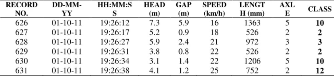
As an illustration, Figure 6 below displays vehicle sequence combination number 8, i.e. the sequence of vehicle class 2 (2-axle truck), class 12 (bus or
Logarithmic PDF Θ = 0.71115
coach), class 10 (trailer truck), and class 3 (3-axle truck). This sequence combination has also been verified in the WIM measurement result, which contained similar vehicle sequences in the time series data, as can be seen in Table 5.
Table 4 Vehicle sequence combinations from Monte Carlo simulation. No Vehicle class Comb. No Vehicle class Comb . No Vehicle class Comb. 1 1 1 35 2 7 67 5 13 2 3 36 12 68 12 3 1 37 1 69 1 4 2 38 12 70 3 5 1 39 1 71 1 14 6 1 40 2 8 72 1 7 2 2 41 12 73 2 8 1 42 10 74 12 9 2 43 3 75 1 10 12 44 1 9 76 2 15 11 1 45 1 77 1 12 1 3 46 2 78 1 13 1 47 12 79 1 14 1 48 1 80 1 15 3 49 2 10 81 12 16 16 1 50 1 82 1 17 1 51 1 83 1 18 1 4 52 1 84 2 19 1 53 1 85 1 20 1 54 1 86 1 17 21 10 55 1 11 87 8 22 1 56 1 88 1 23 2 5 57 2 89 1 24 1 58 1 90 1 25 1 59 1 91 2 18 26 1 60 2 92 1 27 1 61 1 12 93 1 28 1 62 1 94 1 29 1 6 63 2 95 1 30 1 64 2 96 1 31 1 65 2 97 1 19 32 3 66 1 98 1 33 1 99 1 34 2 100 2
Figure 6 Vehicle sequences combination number 8.
Table 5 Verification of vehicle sequence combinations from WIM measurements. RECORD NO. DD-MM-YY HH:MM:S S HEAD (m) GAP (m) SPEED (km/h) LENGT H (mm) AXL E CLASS 626 01-10-11 19:26:12 7.3 5.9 16 1363 5 10 627 01-10-11 19:26:17 5.2 0.9 18 526 2 2 628 01-10-11 19:26:27 5.9 2.4 21 972 3 3 629 01-10-11 19:26:31 3.8 0.8 22 526 2 2 630 01-10-11 19:26:34 3.1 1.4 22 1206 5 10 631 01-10-11 19:26:38 4.1 1.2 25 752 2 12
Notes: DD: Day, MM: Month, YY: Year, HH: Hour, MM: Minute, SS: Second
4
Analysis and Discussion
Structure Modeling
4.1
The modeling of a 25 m Bina Marga standard simple span bridge structure (reinforced concrete T-girders), with a 9 m bridge width consisting of 7 m traffic lanes and 1 m sidewalks on both sides [8], was done using 3 dimensional modeling in SAP2000 software, version 14.2.2, as shown in Figure 7. The nominal properties of the bridge’s structure material were: concrete with compression strength fc’ 20 MPa, unit weight (γ) 2400 kg/m3, and a
reinforcement bar with yield strength (fy) 300 MPa, Young modulus (E) 200000
MPa.
Structure Loading
4.2
The loads applied on the bridge structure model were dead load and live load. The dead load consisted of the structure’s self-weight along with the nominal unit weight of reinforced concrete (γ) 2400 kg/m3, superimposed dead load (SIDL) of a 100-mm asphalt layer with nominal unit weight (γ) 2400 kg/m3, and a concrete side barrier. The live load for this model consisted of the WIM measured vehicular live load sample with the vehicle combination sequences that were determined in Section 3.3 using 1000 vehicular live load samples
from a Monte Carlo simulation based on the PDF of each axle load class as determined in Section 3.2.
(a) Plan view of the bridge
(b) Side view of the bridge
(c) Cross-section of the bridge
Figure 7 Structure modeling of the bridge.
(a) Class 2 (2-axle truck) (b) Class 12 (bus or coach)
(c) Class 3 (3-axle truck) (d) Class 10 (trailer truck)
Figure 8 Load assignment: vehicle sequence combination number 8 based on WIM measured load.
As an illustration of the WIM vehicular live load assignment to the bridge structure model, a sequence combination consisting of class 2 (2-axle truck), class 12 (bus or coach), class 10 (trailer truck), and class 3 (3-axle truck) was assigned to the bridge structure model according to the position of the tire contact area on the bridge slab for both lanes, as shown in Figure 8. After the vehicular load was assigned to the model, the vehicle loads were combined using superposition to get the vehicular load combination sequences. Then, the 1000 WIM vehicular load sample data for each axle load class were inputted as WIM vehicular live load variation assignment.
For the purpose of comparison, the vehicular nominal load according to RSNI T-02-2005, consisting of lane load D and truck load T, was also assigned to the bridge structure model. For this bridge with a 25 m span length, according to RSNI T-02-2005, the lane load (D) is uniform distributed load (UDL) 9 kN/m2 plus knife equivalent load (KEL) 49 kN/m, while the truck load (T) is one standard truck with a total weight of 500 kN, as displayed in Figure 9.
(a) “D” Lane load: KEL 49 kN/m
(b) “D” Lane load: UDL (black: 9 kN/m2, grey: 4.5 kN/m2, white: 0)
(c) “T” Truck Load (moving load on two lane) (black: Truck lane 1, grey: Truck lane 2)
Figure 9 Lane load (D) and truck load (T) based on RSNI T-02-2005.
Structure Response: Maximum Bending Moment on Girders
4.3
From the structure response of the structural analysis due to the applied WIM measured vehicular live load, one maximum bending moment value for all girders on the bridge was taken for one value of the load sample variation out of the total of 1000 samples and one vehicle sequence combination out of 19 combinations. For all 1000 samples and 19 combinations, from the Monte Carlo simulation of the WIM measured vehicular live load, the results were 19000
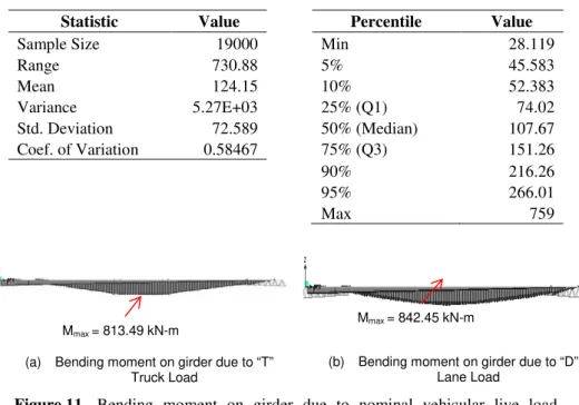
data of maximum bending moment on the girders as random variable, with PDF as shown in Figure 10 and statistic data properties as shown in Table 6. The structure response as maximum bending moment on the girders due to vehicular nominal loads according to RSNI T-02-2005 is displayed in Figure 11.
Figure 10 PDF of maximum bending moment on girder due to WIM measured vehicular live load.
Table 6 Statistic data properties of maximum bending moment on girder due to WIM measured vehicular live load.
Statistic Value Percentile Value
Sample Size 19000 Min 28.119
Range 730.88 5% 45.583 Mean 124.15 10% 52.383 Variance 5.27E+03 25% (Q1) 74.02 Std. Deviation 72.589 50% (Median) 107.67 Coef. of Variation 0.58467 75% (Q3) 151.26 90% 216.26 95% 266.01 Max 759
(a) Bending moment on girder due to “T” Truck Load
(b) Bending moment on girder due to “D” Lane Load
Figure 11 Bending moment on girder due to nominal vehicular live load according to RSNI T-02-2005. Lognormal PDF σ = 0.52908 μ = 4.6782 Mmax = 813.49 kN-m Mmax = 842.45 kN-m
From the maximum bending moment on the girders due to the vehicular nominal load according to RSNI T-02-2005, the lane load (D) and truck load (T) are as displayed in Figure 11 and tabulated in Table 7, the lane load governing the vehicular nominal load for this 25 m bridge with maximum bending moment at 842.45 kN-m. The ratio of nominal value of maximum bending moment (RSNI T-02-2005) to average value of maximum bending moment (WIM measurement) was 6.81. The probability of the nominal maximum bending moment value (RSNI T-02-2005) exceeding the distribution of maximum bending moment due to the WIM measured vehicle live load was 5 x 10⁻⁵. This can be an indication, within the scope of this work, that the nominal value of the vehicular live load according to RSNI T-02-2005 is conservative, because usually the nominal live load value can be taken with a probability of exceedance of about 5% from the PDF of the measured live load. However, in deciding if the nominal live load value is conservative or not, the reliability index according to an LRFD based bridge design code must be the main consideration. Hence, a reliability analysis is needed to determine the reliability index or structure probability of failure due to the WIM measured vehicular live load data.
Table 7 Probability of maximum bending moment on girder due to RSNI T-02-2005 vehicular nominal live load exceeded by WIM measured vehicle load.
Load M (kN-m) Cumulative Density (F(x)) 1-F(x) D 842.45 0.99995 5.0E-05 T 813.49 0.99993 6.6E-05
Reliability Analysis: Reliability Index Evaluation
4.4
In the reliability analysis, three variables were used – resistance (R), dead load (D), and live load (L) in terms of bending moment (kN-m) – in order to calculate the reliability index (β) with performance function R-D-L > 0, but there were non-normal variables within R, D, and L. The equivalent normal distribution method (Rosenblatt, 1952) can be used by doing a Rossenblatt transformation of non-normal distribution into the equivalent normal distribution. The L variable was known as lognormal from the previous GOF test, R is lognormal [5], and D is normal [5]. The equation used for calculating the reliability index (β) is:
𝛽= 𝜇𝑅𝑁−𝜇𝐷−𝜇𝐿𝑁
�(𝜎𝑅𝑁)2+(σ𝐷)2+�𝜎𝐿𝑁�2
(1) where:
𝜇𝑅𝑁 mean value of equivalent normal R variable 𝜇𝐷 mean value of D variable
𝜇𝐿𝑁 mean value of equivalent normal L variable 𝜎𝑅𝑁 standard deviation of equivalent normal R variable σ𝐷 standard deviation of D variable
𝜎𝐿𝑁 standard deviation of equivalent normal L variable
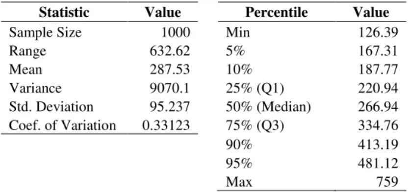
Figure 12 PDF of maximum bending moment on girder due to maximum probable WIM measured vehicular sequence loading combination.
Table 8 Statistic Data properties of maximum bending moment on girder due to maximum probable WIM measured vehicular sequence combination loading.
Statistic Value Percentile Value
Sample Size 1000 Min 126.39
Range 632.62 5% 167.31 Mean 287.53 10% 187.77 Variance 9070.1 25% (Q1) 220.94 Std. Deviation 95.237 50% (Median) 266.94 Coef. of Variation 0.33123 75% (Q3) 334.76 90% 413.19 95% 481.12 Max 759
The live load variable (L) was taken from the WIM measured vehicular live load for the maximum probable vehicle sequence combination loading, which was combination number 8. This combination is the sequence of vehicle class 2 (2-axle truck), class 12 (bus or coach), class 10 (trailer truck), and class 3 (3-axle truck). This maximum load effect on the girders had a lognormal distribution as displayed in Figure 12 with average value (μL) 287.53 kN-m,
standard deviation (σL) 95.24 kN-m, and coefficient of variance / c.o.v. (ΩL)
0.33 as summarized in Table 8. Dead load (D) was taken from the structure analysis due to dead load and SIDL, with nominal value bending moment on the girders (Dn) at 1651.13 kN-m. The bias factor and c.o.v. (ΩD) of the dead load
Lognormal PDF σ = 0.30943 μ = 5.6119
were 1.05 and 0.10 respectively [5]. Hence, the average bending moment on the girders due to dead load and SIDL, (μD), and its standard deviation (σD) were
1733.68 kN-m and 173.37 kN-m respectively.
The resistance variable R was taken as the bending moment capacity of the girders, which was determined by using the bending moment capacity equation that considers the uncertainty in the equation due to random variables such as steel bar properties fy , concrete strength fc’, and also steel bar area As. The
coefficient of variance c.o.v.As was assumed to be 3% and non-biased, the ratio
of nominal value to average value, vAs, was assumed to be 1. The nominal value
of concrete strength and steel bar strength was assumed to be 5%, in the lower-tailof each normal distribution, the c.o.v. of steel bar strength was 15% and the
c.o.v. of concrete strength was 20%. The results from this bending moment capacity variable calculation with uncertainty analysis were: average value (μR)
was 6676.98 kN-m, standard deviation (σR) was 1597.63 kN-m, and coefficient
c.o.v. (ΩR) was 0.24.
In a Rossenblatt transformation, the lognormal distribution parameters of L and
R must be determined. Then, using these two equations (example for L only), the average value and standard deviation of equivalent normal L and R can be determined.
𝜎𝐿𝑁=𝑙∗𝜉𝐿 (2)
𝜇𝐿𝑁 =𝑙∗(1−ln(𝑙∗) +𝜆𝐿) (3)
To determine the reliability index, iteration calculation is necessary because there are variables with non-normal distribution: R and L are lognormal. Although the equation is a linear performance function, the average value and standard deviation of non-normal variables are unknown, since it is a function of each failure point value. The iteration procedure for calculating the reliability index until its convergence is displayed in Table 9 (in terms of bending moment, kN-m). For the first iteration, the failure point value is assumed as the average value of L and R. From Table 9, the reliability index 𝛽 is 4.68 with corresponding probability of failure 𝑝𝐹 is 1.42 x 10⁻⁶.
An LRFD-based bridge standard for structure design or loading must have a reliability target that constrains factors such as load and resistance. AASHTO has a target reliability index β of 3.50 or probability of failure 𝑝𝐹 of 2.32 x 10⁻⁴. As an alternative for AASHTO, Nowak [7] recommends a target reliability index β of 3.72 for a bridge with a life time of 50 years, with probability of failure 𝑝𝐹 is 10-4.
From the reliability analysis, the resulted reliability index 𝛽 was higher than the target reliability 𝛽 of AASHTO based on RSNI T-02-2005 (3.50) and also higher than the target reliability 𝛽 of 3.75 recommended by Nowak. This can be an indication that the bridge has a smaller risk of failure than targeted, which makes it conservative. Therefore it can be concluded that, within the scope of this work, the nominal vehicular live load provision in the Indonesian bridge loading code RSNI T-02-2005 is conservative.
Table 9 Reliability index β iteration procedure.
Iteration Failure points σ i N μi N β l* r* σL N σR N μL N μR N 1 123.74 6760.56 39.93 1595.17 221.63 6572.37 2.877 2 126.60 2012.04 40.85 474.74 223.86 4394.53 4.806 3 239.67 2258.25 77.33 532.84 270.83 4671.59 4.715 4 320.68 2304.91 103.47 543.85 269.00 4720.98 4.686 5 355.47 2331.93 114.69 550.22 261.57 4749.15 4.682 6 366.28 2339.22 118.18 551.94 258.55 4756.69 4.682 7 369.29 2341.28 119.15 552.43 257.65 4758.82 4.682 8 370.09 2341.82 119.41 552.56 257.41 4759.38 4.682 9 370.30 2341.96 119.48 552.59 257.34 4759.53 4.682 10 370.36 2342.00 119.50 552.60 257.33 4759.56 4.682
5
Conclusion
The number of WIM measured vehicles live load data used in this study was 72353, classified into twelve different classes using the EURO13 classification. As expected, the measured vehicular load values varied, even when they came from the same vehicle class. For example, if the truck vehicular nominal load (T) from RSNI T-02-2005 was defined according to a 3-axle vehicle with total load 500 kN, then the 3-axle truck (class 3) from the WIM measured total vehicle load varied from 17.5 kN to 339.8 kN with coefficient of variation (c.o.v) is 0.34. As expected, this can be an indication that the nominal value of the vehicular load is different for various actual WIM measured vehicular load results, since nominal vehicular loads can be taken as one value to simplify the design procedure as long as the design is within acceptable risk criteria.
The maximum bending moment on the 25 m reinforced concrete bridge girders due to the applied vehicular nominal load according to the bridge loading standard from RSNI T-02-2005 was 842.45 kN-m, with the ratio of nominal value of maximum bending moment from RSNI T-02-2005 to average value of maximum bending moment of WIM measurement at 6.81. The probability of the nominal maximum bending moment value (RSNI T-02-2005) exceeding the
distribution of maximum bending moment due to the WIM measured vehicle live load was 5 x 10⁻⁵.
The reliability index (𝛽) of the 25 m reinforced concrete bridge girders due to the WIM measured vehicular live load was 4.68 with corresponding probability of failure 𝑝𝐹 of 1.42 x 10⁻⁶. This is higher than the target reliability 𝛽 of AASHTO (based on RSNI T-02-2005) of 3.50 and also higher than the target reliability 𝛽 of 3.75 recommended by Nowak [7]. This can be an indication that the bridge has a smaller risk of failure than targeted (=�1/382 ratio of pF 10
-4
), which is conservative enough for bridge structure design.
Acknowledgements
The weigh-in-motion vehicular load measurements and bridge structural data reported herein were taken by researchers from the Institute of Road Engineering (IRE), Ministry of Public Works, Republic of Indonesia. The authors would like to thank Mr. IGW Samsi Gunarta, Head of Laboratory, Traffic and Environmental Research (TERL) IRE, and also Mr. Untung Cahyadi and Mr. Redrik Irawan as IRE researchers for the data and information that this study was based upon.
References
[1] Ellingwood, B. R., Reliability-based Condition Assessment and LRFD for Existing Structures, Structural Safety, 18(2/3), pp. 67-80, 1996.
[2] National Standardization Agency of Indonesia, RSNI T-02-2005: Bridge Loading Standard, 16-25, 2005. (Text in Indonesian)
[3] Nowak, A.S., Calibration of LRFD Bridge Design Guide, NCHRP
Report 368, pp. 37-125, 1999.
[4] Institute of Road Engineering Ministry of Public Works, Technical
Report of Vehicular Load Survey using WIM Method in Cikampek-Pamanukan Road, 2011.
[5] Ang, A.H-S., & Tang, W.H., Probability Concepts in Engineering
Planning and Design Volume II - Decision, Risk, and Reliability. John Wiley and Sons, Inc., pp. 274-435, 1984.
[6] AASHTO, AASHTO LRFD Bridge Design Specifications, 6th ed., Section 3, American Association of State Highway and Transportation Officials, Washington DC, USA, pp. 17-36, 2012.
[7] Nowak, A.S., Reliability-based Calibration of Bridge Design Code,
University of Nebraska-Lincoln, pp. 3-74, 2007.
[8]
Directorate General of Highways, Department of Public Works,
Republic of Indonesia. Reference No.04/BM/2005:
Standard of
Drawings for Road and Bridge Works,
Volume II
, 2005. (Text in
Indonesian)
[9] Palczewski, J., & Palczewski, A., Monte Carlo Simulation Lecture Notes, Uniwersytetu Warzawskiego, pp.1-54, 2014.