prediction interfaces
Alexey Dmitrenko
School of Science
Thesis submitted for examination for the degree of Master of Science in Security and Mobile Computing.
Espoo June 26, 2018
Supervisors
Prof. N. Asokan, Aalto University Prof. Danilo Gligoroski, NTNU Advisors
M.Sc. (Tech) Mika Juuti PhD Samuel Marchal
Abstract of the master’s thesis
Author Alexey Dmitrenko
Title DNN model extraction attacks using prediction interfaces
Degree programme Security and Mobile Computing
Major Security and Mobile Computing Code of major T3011
Supervisors Prof. N. Asokan, Aalto University Prof. Danilo Gligoroski, NTNU
Advisors M.Sc. (Tech) Mika Juuti, PhD Samuel Marchal
Date June 26, 2018 Number of pages 68 Language English
Abstract
Machine learning (ML) and deep learning methods have become common and publicly available, while ML security to date struggles to cope with rising threats. One rising threat is model extraction attacks where adversaries are able to reproduce a target model close to perfection. The attack is widely deployable since the attacker needs only to have access to predictions to perform this attack. Stolen ML models could either be used for personal advantage to abuse paid prediction services or to create transferable adversarial examples that can be used to undermine the integrity of prediction services, i.e. prediction quality. This is a significant threat in several application areas, such as in autonomous driving, which rely heavily of computer vision via deep neural networks.
In this thesis, we reproduce existing model extraction attacks and evaluate novel techniques to extract deep neural network (DNN) classifiers. We introduce new synthetic query generation strategies, and demonstrate their efficiency at extracting models for creating transferable targeted adversarial examples from stolen DNNs.
Preface
The thesis work was done by the author under the guidance of Professor N. Asokan of Aalto University, Professor Danilo Gligoroski of NTNU and my advisors at Aalto University M.Sc. (Tech) Mika Juuti and PhD Samuel Marchal. I would like to express my sincerest gratitude and appreciation to Mr. Mika Juuti, Mr. Samuel Marchal and Professor N. Asokan for their extended guidance, valuable comments and feedback throughout the thesis.
Otaniemi, 26.06.2018
Contents
Abstract 2 Preface 3 Contents 4 1 Introduction 8 1.1 Motivation . . . 8 1.2 Contribution. . . 9 1.3 Structure . . . 10 2 Background 11 2.1 Mathematical background . . . 11 2.1.1 Convolution . . . 11 2.1.2 Gradient . . . 11 2.1.3 Chain rule . . . 11 2.1.4 Jacobian matrix . . . 12 2.1.5 p-norm . . . 12 2.1.6 Lp space . . . . 12 2.2 Machine Learning . . . 14 2.2.1 Training ML model . . . 14 2.2.2 Activation functions . . . 162.2.3 Evaluating supervised ML models . . . 17
2.3 Neural Networks . . . 18
2.4 Machine-Learning-as-a-Service platforms . . . 19
2.5 Adversarial Machine Learning . . . 19
2.5.1 Adversarial examples . . . 20
2.6 Model extraction attacks . . . 23
2.6.1 Tramer attack . . . 23
2.6.2 Papernot attack . . . 24
2.7 Technical background . . . 25
2.7.1 Pytorch . . . 25
3 Problem Statement 27
3.1 Threat Model . . . 27
3.2 Requirements . . . 29
4 Methodology 31 4.1 Attacker model learning strategies . . . 32
4.2 Synthetic sample generation . . . 34
4.2.1 Jb-star approach . . . 34
4.2.2 Jb-Top-k approach . . . 35
4.2.3 Jb-self approach . . . 36
4.3 Evaluation of model extraction . . . 36
4.3.1 F-agreement . . . 36
4.3.2 Transferability rate . . . 36
5 Datasets and experimental setups 38 5.1 Mixed National Institute of Standards and Technology (MNIST) . . . 38
5.2 German Traffic Signs Recognition Benchmark (GTSRB) . . . 39
5.3 Experimental setup . . . 42
5.3.1 Ideal server . . . 42
5.3.2 Dedicated hardware-supported prediction API . . . 43
6 Evaluation 45 6.1 Evaluation setup . . . 45
6.2 Ideal Server: DNN extraction performance . . . 47
6.2.1 Attacker set size . . . 47
6.2.2 Training time . . . 49
6.2.3 Comparison with state-of-the-art . . . 51
6.2.4 Impact of ϵ value. . . 52
6.2.5 Synthetic query impact . . . 53
6.2.6 Impact of learning strategies . . . 56
6.3 Hardware prediction API: Movidius Neural Compute Stick . . . 58
6.4 Challenges . . . 59
7 Related work 61 7.1 ML model extraction attacks . . . 61
8 Conclusion 63 8.1 Summary . . . 63 8.2 Future work . . . 64
Abbreviations
API Application Programming Interface
CNN Convolutional Neural Network
DNN Deep Neural Network
FGSM Fast Gradient Sign Method
GPU Graphics Processing Unit
ML Machine Learning
MLaaS Machine-Learning-as-a-Service
NCS Neural Compute Stick
PGD Projected Gradient Descent
ReLU Rectified Linear Unit
VPU Vision Processing Unit
1.1
Motivation
Machine learning (ML) is increasingly being deployed by many companies and start-ups as part of the everything-as-a-service (XaaS) paradigm [3, 32, 14]. Machine Learning-as-a-Service (MLaaS) is a new service concept that pushes machine learning model prediction, and sometimes training too, into the cloud. The market slice is expected to grow rapidly in the coming five years. For example, according to the MarketsandMarketsTM the MLaaS market is estimated to grow from USD 613.4
Million in 2016 to USD 3,755.0 Million by 2021 [29]. This increase is expected to happen due to a change in availability and price of ML services. Before, only a few companies had enough data and know-how to use Machine Learning for large datasets. With the introduction of MLaaS, it is possible for everyone to use such services and without hardware concerns. For providers, it is also beneficial because it becomes a new business field that companies can monetize.
Recent changes in data protection regulation (i.e General Data Protection Regu-lation, GDPR) [9] introduced several difficulties for ML. GDPR requires all decision made by machine algorithm to be clearly explained ("right to explanation" [6]) making it difficult to deploy deep learning techniques due to their complexity and non-linear decisions. Exposure of certain models to data leakage and theft are serious threats. For example, banks and other financial institutes that use ML methods to decide whether a person is eligible for a mortgage now should explain why a particular decision is made. Therefore, a clever adversary can exploit such fact and try to use this information from numerous applications to infer decision boundaries of the financial model and gain financial advantage of it.
There are several other problems in ML that are related to information security. In case of a health-care system, for example, models process patient data and it should be kept private. However, there are ways to disclose such information if no security measures are applied to algorithms [41, 7]. Other security vulnerabilities in machine learning are related to SPAM filters, network security software, security information event management systems and other types of classifier systems. If an adversary manages to obtain information about the model that is used in any of these applications, then he may try to execute an evasion attack, to evade detection by such a system. In the evasion attack scenario, a malicious user typically tries to add
adversarial perturbation to natural samples which are misclassified by the model [36, 35]. Such samples can violate service usability or model integrity (prediction quality). Evasion attacks are not the only threat in exposing ML models. There are also inversion attacks where the goal of an adversary is to obtain a part of a training set via analysis of a ML model.
Undoubtedly, all these issues can happen whether systems are deployed using company resources in a company network, or if they are in the cloud infrastructure on an untrusted third-party server. However, threats against ML systems apply not only when in the cloud settings, but in locally available models as well. In fact, the threat surface increases when the attacker has access to the model, meaning that the attacker can do more powerful attacks. For instance, with the huge popularity of IoT devices and smart infrastructures, ML models are widely deployed inside hardware processing units. For example, Vision Processing Unit (VPU) from Intel Movidius is extensively used in security cameras1. These hardware chips are designed to accelerate deployability of machine intelligence by having low power consumption. Because of concerns about misuse of the models they are expected to be hardware-protected by a Trusted Execution Environment e.g. Intel SGX [39]. Be it as it may, prediction APIs will always be queryable in such models for practical reasons. As we discuss in this work, an adversary only needs access to the prediction API in order to perform model extraction attacks. In this thesis, we analyze the applicability of model extraction attacks on DNNs and propose novel attacks. The main goal is to understand the risk of model extraction attacks for service providers and its applicability in real scenarios.
1.2
Contribution
In this thesis we claim the following contributions:
• We reproduce previous state-of-the-art attack methods [41, 36]. We evaluate the attack effectiveness of previous techniques and isolate several variables that contribute to the effectiveness of model extraction (Section 6). We analyze the effect of each separately. We validate their performance on both previously reported and additional dataset [36] (Section 2.6).
• We propose novel query strategies along with the algorithm to extract DNN
models using only prediction APIs. The method extends previous work [36] (Section 4).
• We test and evaluate proposed techniques to steal DNNs on a neural compute device (embedded system). We show that extraction of local models is feasible (Section 6).
1.3
Structure
The remainder of the work is structured as follows: Section 2 provides with basic descriptions of algorithms and definitions that are used throughout this work. We give an overview of previous attacks that used as a baseline in the evaluation. Section3 presents the problems discussed in this thesis, identifies the threat model and lists requirements for new DNN extraction techniques. Section 4 introduces a generic approach to extract a ML model and describes our new query strategy to improve existing attacks. Section5 presents datasets used for evaluation of the attack along with different learning strategies for the attack algorithm that we propose will have a positive impact on the extraction of DNN models. Section5.3 gives an overview of experimental setups that we use to evaluate our work and describes DNN architectures we used. Section6gives an overview of performance metrics that are used to evaluate previous attacks as well as new methods, shows the evaluation of initial samples impact, synthetic query impact, training strategy impact and the effect of varying training time of proposed solution and previous attacks. Section 7 discusses the related work to DNN model extraction and defenses to date. We conclude this thesis by presenting conclusions and describing possible future work in Section 8.
2
Background
In this section, we address all the necessary definitions of terms, techniques that are closely related to the thesis. We present definitions of important concepts in order to give a better understanding of the solutions and evaluations described in this work.
2.1
Mathematical background
2.1.1 ConvolutionConvolution is a mathematical operation applied on two functions f and g that produces a third function f ∗g. Usually, the result of the convolution considered to be an altered version of f or g. The convolution operation can be interpreted as the "similarity" of one function to the reflected and shifted copy of another. In other words, assume f, g : Rd →
R are integrable functions in Rd. Therefore, the
convolution of those functions is f ∗g : Rd →
R and it can be described as the
following mathematical expression:
(f ∗g)(x) = ∫ Rd f(y)×g(x−y)dy= ∫ Rd f(x−y)×g(y)dy (1) 2.1.2 Gradient
Gradient∇is a vector that indicates the direction of the greatest increase of a certain value ϕ. The absolute value of a gradient ∇ϕ is equal to the rate of growth of this value in this direction. It can be described with following mathematical expression:
∇ϕ= ∂ϕ ∂x ×i+ ∂ϕ ∂y ×j+ ∂ϕ ∂z ×k (2)
Wherei,jandkare unit vectors in the directions ofx, y andzaxis correspondingly.
2.1.3 Chain rule
Chain rule allows computing the derivative of the composition of two or more functions. Consider functionf is differentiable at a point x0 and a function g is differentiable
at a pointy0 =f(x0), thus their composition h=f ◦g is also differentiable at that
point and its derivative is equal to
h′(x0) =g′
(
f(x0)
)
2.1.4 Jacobian matrix
Jacobian matrix is a matrix that consists of gradient values of a function f [8]. If a function f is differentiable at a pointx and have all partial derivatives at x then there is a Jacobian matrix J that shows linear approximation off near the point x. It can be described as the following mathematical expression:
J= df dx = [ ∂f ∂x1 · · · ∂f ∂xn ] = ⎡ ⎢ ⎢ ⎢ ⎣ ∂f1 ∂x1 · · · ∂f1 ∂xn .. . . .. ... ∂fm ∂x1 · · · ∂fm ∂xn ⎤ ⎥ ⎥ ⎥ ⎦ (4) 2.1.5 p-norm
A norm is a function that is defined on a vector space and generalizes the definition of vector length and absolute value. The norm of a vectorV over a field of real (R) numbers can be described as a functionp:V →R that has following properties:
1. p(x) = 0 =⇒ x= 0V;
2.∀x, y ∈V, p(x+y)≤p(x) +p(y); 3.∀α ∈R,∀x∈V, p(αx) = |α|p(x).
(5)
These properties are called the norm’s postulates [1]. Usually, norms are written as∥ · ∥p and defined as:
∥v∥p = ( n ∑ i=1 |vi|p )1p (6)
The most commonly used norm in R space is the Euclidean norm orL2 norm. It
has the following expression: ∥X∥2 =
√ (
x2
1+· · ·+x2n )
, wherenis the dimensionality of X. It is commonly seen as an expression describing the length of a vector.
2.1.6 Lp space
Lp space is a mathematical function space that is defined using p-norm in finite dimensions [1]. Often it is used as a distance metric between two objects inLp space. The most common distance metrics usingLp norm in machine learning areL0, L1, L2 and L∞ General formulas for Lp distances can be written as∥x−x′∥p.
• L0 distance for vector x and x′ assesses the number of elements that differ.
For example, in case of images, it shows the total number of pixels which are different in one image comparing to the other
• L1 distance for vectorx andx′ assesses the summed absolute value discrepancy
between xandx′. In case of images, it is the sum over all pixels absolute value discrepancies.
• L2 distance for vectorxandx′ assesses Euclidean distance between two objects.
It is the most common distance metric in small-dimensional space (n≤3), but it loses its practical usefulness in high-dimensional space (n≥3). It was shown in [2] that as the n increases the Euclidean distance between a point and its closest neighbor, and between that point and its furthest neighbor changes in non-obvious way affecting the results.
• L∞ for vector x and x′ assesses the maximum change in any dimension. ∥x−
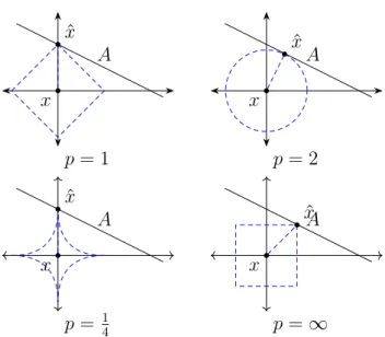
x′∥∞= max(|x1−x′1|, ...,|xn−x′n|), where xi denotesx’s value in dimension i. In images it means that the discrepancy value between two images is always limited to some maximum value, but at the same time, any number of pixels may be modified. A A x ˆ x x ˆ x p= 1 p= 2 A A x ˆ x x ˆ x p= 14 p=∞
Figure 1: P-space graphical representation with unit circles.
Graphical representation ofLp space forp in [1,2,14,∞] using unit circles can be found in Figure 1. The dashed shapes denote equal distance from origin in different
Lp spaces. The case when 0≤ p <1 is different and Equation 6 is not applicable. The vector space in this case is not locally convex and the same formula cannot be applied. There is a distance metric instead that defines the case when 0 ≤p < 1,
that is dp(x, y) = n ∑ i=1 |xi−yi|p (7)
Therefore, we show p= 14 as an example for simplicity. Lower values of p converge to axis lines and are hard to represent on the graph.
2.2
Machine Learning
ML is a subclass of artificial intelligence methods. The main characteristic of ML is not to provide a direct solution to a particular problem, but to do so-called learning while solving a great number of similar problems. Training occurs with the use of mathematical statistics, numerical methods, optimization methods, probability theory, graph theory, and various techniques of working with data in digital form. Training is commonly divided into two types:
1. Supervised learning or learning from examples, is a type of training based on inductive learning and identification of empirical regularities in the data. Many methods are closely related to information extraction and data mining techniques.
2. Unsupervised learning (self-learning, spontaneous learning) is the type of training describing internal interrelations, dependencies and regularities existing between objects.
Unsupervised learning is often contrasted with supervised learning, where each learning object is forced to have a "correct answer" and there is a need to find a relationship between the system’s stimuli and responses.
Classification, the area of predicting categorized labels of samples, is the most common form of supervised learning. A great deal of real-world problems can be cast as classification problems. For instance, classifying digits and traffic signs are fundamentally the same problem, and can be solved with similar algorithms. We will focus on supervised techniques in this thesis.
2.2.1 Training ML model
In order to train a ML model one need to find optimal parametersθ that minimize a classification error rate. Usually, the error rate described by cost functionC. Overall, the goal of training is to minimize a function C by finding an optimal point θ that
solves ∂Cθ(θ) = 0. However, it is mathematically infeasible to find the solutions of this equation so instead numerical optimization methods are applied during training. The most common supervised learning optimization method to train a ML model is a gradient descent. Gradient descent is an iterative method of finding local minimum of a function C using gradient of that function. The method takes steps towards the negative gradient of a function at a pointθ. One step can be viewed as the following mathematical expression:
θk+1 =θk−λ× ∇C(θk) (8) Where λ corresponds to a chosen learning rate and describes a step size of the algorithm. However, training suffers from overfitting, the phenomenon when the trained model explains well the examples from the training set, but it works relatively poorly on the examples that did not participate in the training (on the examples from the test set). In other words, overfitting in most cases occurs when the resulting polynomials have too large coefficients. Accordingly, this can be dealt with in a rather natural way by adding a penalty to the target function, which would punish the model for too large coefficients. Regularization is the most common method to solve overfitting problem.
Regularization is a method of adding some additional information during training phase to network parameters to prevent overfitting. This information often has the form of a penalty for the complexity of the model. For example, it can be constraints on the smoothness of the resulting function or constraints on the norm of vector space.
There are many ways to apply regularization in statistics and ML. We describe three most common and widely used, such as L1, L2 regularization penalty and
dropout.
L1 regularizationis a way to addL1 distance term (absolute value of magnitude)
to loss function as a penalty. It can be described with the following formula
L1 = ∑ i Ci(θi) +λr ∑ i |θi| (9)
where C is the cost function, λr is regularization coefficient and θi corresponds to the parameters of the network.
L2 regularizationapplies 2-norm constraints to the cost functionC as a penalty.
It can be described with the following formula.
L2 = ∑ i Ci(θi) +λr ∑ i θi2 (10)
Dropoutis the method of regularization of ML models that is designed to reduce overfitting of the model. The essence of the method is that in the learning process, a layer is selected from which a certain number of neurons (for example 50%) are randomly emitted, further calculations are turned off. This technique improves learning efficiency and the quality of the result [16]. More trained neurons gain more weight in the network [40].
2.2.2 Activation functions
Activation functions are used to define the output of a neuron. We consider Rectified Linear Units (ReLU) and Softmax activation functions in this thesis.
ReLU is the activation function that takes only positive part of its argument. It can be described as the following formula:
f(x) = x+= max(0, x) (11) wherex is the input to the function. This activation function shows better perfor-mance in training of deep networks than the previous popular choices, e.g. hyperbolic tangent, logistic sigmoid [12].
Softmax is the activation function that converts a vector z of dimension K to a K-dimensional vectorσ, where each coordinateσiof the resulting vector is represented by a real number in the interval [0,1] and the sum of coordinates is 1. Therefore, it is used to represent probability distribution and usually applied at the last layer of the network to get the probabilities as predictions. It can be described as the following formula σ(z)i = ezi ∑K k= 1ezk (12)
2.2.3 Evaluating supervised ML models
The goal of any ML model is to learn general trends in data that will perform well on an unseen data. Once the training is done it is important to evaluate the performance of the model on new examples that were not used during the training of the model. There are several performance metrics. For supervised models, the most popular and simple metric isaccuracy. A model’s accuracy is a fraction of right predictions on unseen test data (held-out data) that match theactual labels (ground truth data) to the total number of samples in the test set. It shows how well the model is able to generalize patterns in the data and not to memorize it. However, accuracy loses its practicality if the dataset is unbalanced. It no longer can show a true picture of how the model performs in a multi-class scenario where label distribution is uneven across several classes. In this case, the performance metric needs to treat each class equally and show how well the model performed on average no matter class distribution.
Precision corresponds to the ratio of true positive values (correctly labeled) and total number of true positives and false positives (incorrectly labeled) tp+tpf p. It shows the classifier’s accuracy when claiming a sample is a member of the positive class.
Recall corresponds to the ratio of true positive values and the sum of true positives and false negatives tp+tpf n. It shows the classifier’s capability to identify all positive samples.
F-score is the harmonic mean of precision and recall. F-score is calculated with the following mathematical expression:
F = 2×
(precision×recall
precision+recall
)
(13)
F-score reaches its best value at 1 and worst at 0. Initially, F-score is for binary classification. However, it can be applied to multi-class scenario as well by calculating F-score values for each class with respect to the rest and average it across all classes (macro-averaged) F-score.
In this thesis we mainly use the macro-averaged F-score agreement (F-agreement) to weight each class equally and get a fair comparison that is independent of label distribution. F-agreement is calculated w.r.t the target model predictions as ground truth data and the attacker model as held out data.
2.3
Neural Networks
In this work, we define a neural network as a mathematical model, as well as its software or hardware implementation. It was originally designed on the principle of organization and functioning of biological neural networks - networks of nerve cells of a living organism. However, a neural network is also viewed as a parameterized function f : X → Y that produces some output y ∈Rm from some input x∈ Rn. As the name suggests, neural networks contain severalneurons. Each neuron in the first layer receives inputs from a set number of sourcesx= [x1, . . . , xn]. These inputs are scaled with a parameterized weight vector and a bias term, the results of which is finally passed through an activation functionσ(·). Therefore, the output of a neuron isf(x, w) =σ(w×x+b). Usually, neurons are combined into layers and layers into networks. Consequently, a deep neural network (DNN), is a hierarchical composition of large number of neurons and layers.
Convolutional Neural Networks (CNN) are DNNs that consists of convolutional neurons and layers. A convolutional neuron is a type of neuron that perform the convolution operation (Section2.1.1) on the input [23]. The main difference from ordinary DNN is that neurons are arranged in several dimensions which makes it efficient to use CNNs on images. That is weights are represented as multi-dimensional matrices and denote as kernel of a convolutional neuron. The most common kernel is a two-dimensional matrix that can be written as 2D kernel. CNN that is using 2D kernels is referred as 2D convolutional CNN. There are also 1D and 3D convolutional CNNs, but these are not used in this thesis. The other difference is that in CNNs parameters are shared and the same depth slice of neurons is computed as convolution of the neuron’s weights across the given input.
Typically a convolutional layer is followed by pooling layer to perform down-sampling of the input. The pooling layer is a unifying convolution neuron with a positive steph that aggregates input data in a rectangle area of sizeh×h. Maximum
and mean are typical aggregate functions. Convolutional layers may also consist of other parameters, such as padding and stride. Stride is the step size of convolutional kernel across the input. Padding controls the output dimensions of the layer. In this work we use two common padding types, "valid" and "same" in particular. "Valid" padding basically means that there is no padding at all. For example, if image dimensions aren×n and kernel size is f×f, the new dimension would be n′×n′, wheren′ =n−f+ 1. In this case no additional padding is applied. However, "same"
padding convolution keeps dimensions of the output at the same value as it was in the input. In this case, padding value is always equal to p = f−21 where f is the convolution kernel size. Typically zeros are padded in the padding operation.
DNNs are typically used with back-propagation [23], a process that is used in gradient descent algorithm (Section 2.2.1) where errors are propagated through the network and the contribution of each parameter of the network is calculated with the chain rule (Section2.1.3). This process allows training of a DNN to incrementally become better at its task.
2.4
Machine-Learning-as-a-Service platforms
Everything-as-a-service (XaaS) is a collective term to describe different as-a-service platforms such as Software-as-a-Service, Platform-as-a-Service, and Infrastructure-as-a-Service. XaaS concept allows mobilizing software across different networks, including ML software. It allows providers to offer a great variety of resources as cloud-based on-demand services to clients. In addition, it opens numerous possibilities to small businesses or individual entrepreneurs, who have a limited budget or resources for a variety of everyday tasks, to move their business to the cloud with high computational power.
For most parts, any technology that can be provided over the Internet and delivered on-site can be included in XaaS [38]. ML is not an exception and has a highly valuable part of this concept due to a nowadays increasing client-side demand for various tasks that need ML.
Machine Learning-as-a-Service (MLaaS) platforms are typically cloud-based in-frastructures that provide web API to train, validate and use ML model. Usually, service providers try to construct their interface in a way that even a non-expert user can understand it. There are many different services for various clients [43].
2.5
Adversarial Machine Learning
Adversarial ML is a research area where ML algorithms and tasks are considered in the presence of an adversary. A clever adversary can modify the input to the model in a way that it compromises some aspect of overall system security, such as confidentiality, integrity or availability. For example, spam filters can be misled by the adversary and label spam message as non-spam or vice versa which will cause a violation of the system’s ability to provide a service as intended.
In the domain of image classification or recognition, an adversary can apply a small change to the image in order to "fool" a target model in the output prediction. There are several techniques to craft such samples. In this work we use the two proposed techniques: Fast Gradient Sign Method and Projected Gradient Descent [13, 30].
2.5.1 Adversarial examples
An adversarial example can be defined as a modified sample of original data that is misclassified by a target ML model while retaining its functionality. Typically, samples are changed with a value (perturbation), so that the samples still very similar to the original image (measured withLp distance Section 2.1.6). The definition of functionality is vague and depends on the use case of a ML task. To give a better understanding consider the following cases:
1. A malware detection software aims to recognize malware and viruses on given input files. An adversary’s goal is to modify a malware sample in a way that it is misclassified by the detection system but the overall functionality of the malware remains the same. In other words, the adversary tries to solve a problem of finding a minimal perturbation applied on the sample that would maintain the intentional ultimate behavior, but also "fool" the detection system at the same time.
2. In image classification models, technically the perturbation size could vary a lot depending on how the system is used. Suppose, we have a system that performs image detection/classification and gives the input image to the user to verify prediction (i.e. online image recognition service, such as Google image search). In that case, the adversarial example would be verified by the human eye which puts some constraints on the adversarial examples crafting (typically in the form of a lower Lp norm). With that scenario, an adversary would need to find the smallest perturbation possible for it to be unnoticeable for the human eye and at the same time fool the detection system.
3. In many image detection/classification models, classification is done without human interaction or verification, such as in real-time prediction of objects from cameras, self-driving cars etc. In these cases, the perturbation applied on the image needs to mislead a target classifier.
Overall, the examples above represent so-called white-box scenarios in which an adversary has access to original model’s internal outputs and can perform back-propagation to calculate gradients. Fooling a target model without access to model internals is considerably more difficult. However, this is the situation in many real scenarios: the adversary may only have access to a prediction API that returns probabilities or labels. That is the so-called black-box attack scenario. In this case, an adversary often needs to first "steal" a model and craft adversarial examples on the attacker model, to find examples that would be misclassified by the attacker model in the hope that the same adversary example would mislead the original model as well. These are referred to as transferable adversarial examples. Papernot et al. [35] studies the transferability property for adversarial examples. In general, the authors introduce an algorithm that exploits adversarial examples transferability in a black-box environment. They explore various algorithms, such as neural networks, logistic regression, support vector machines, decision trees, nearest neighbors, and ensembles and test transferability on the MNIST image dataset using model stealing techniques.
Fast Gradient Sign Method (FGSM) One of the techniques to craft adversarial examples was introduced by Goodfellow et al. [13] is theL∞−boundedattack, which
computes a perturbation at a given point in the direction of the gradient at that point. It modifies the original sample in the following way:
x+ϵ·sign(∇xJ(θ, x, y)) (14) where θ are parameters of a model, xis input to the model, y is original labels that correspond to x, J(θ, x, y) is a cost function used to train machine learning model,∇ operator is the gradient of the cost functionJ represented by the Jacobian,
signis the operation of taking the sign of the input and ϵ is the size of perturbation. Therefore, this method implies that we calculate a gradient of the cost function with respect to the input image. This is similar to model training where we calculate gradient with respect to model parameters and modify them to minimize the loss while keeping input as constant. However, in FGSM we keep parameters constant and try to modify the input image to maximize loss. Afterward, FGSM takes the sign of Jacobian matrix of the result, meaning that Jacobian matrix values will contain -1 for all negative values and +1 for all positive values. Consequently, the distance to the original image is exactlyϵ. As can be seen from Equation 14, it is mandatory
to select some ϵ value that is the parameter that controls the size of perturbation. The resulting weight vector is added to the input image. The produced image x′ is called an adversarial example, if the classification resultf(x) is different from f(x′). FGSM is anuntargeted adversarial example crafting method. It does not result in the creation of a specific class, but only a class other thany. An example of such an image can be found in Figure2.
Figure 2: An illustration of adversarial image using FGSM [13].
Projected Gradient Descent Another technique introduced by [30] is PGD. PGD computes a perturbation using gradient decent in its constraint form iteratively changing the original image towards some target label. Assume a model outputs are some probability distributionP(y|x) over labeled image datax. To craft adversarial example using PGD we try to find a newx′image where the loss function is maximized for a given target label y′. In other words, the output of the algorithm will be a new sample that would be misclassified as a target class. PGD constraints the norm of perturbation and can be used with various norms. Often it uses L∞ box
(∥x−x′∥∞ ≤ϵ) to control perturbation size such that the adversarial example is not
much different from original sample.
Overall, PGD is a multi-step algorithm and repeats similar steps as FGSM until it converges or the number of steps is reached. One step in theL∞-bounded PGD is
shown below:
x′ =x′ +α· ∇xJ(x′, y′)
x′ = clip (x′, x−ϵ, x+ϵ)
where α is a step size in the gradient descent algorithm, clip is a clipping operation that puts all pixel values bigger thanx+ϵ to be exactly x+ϵ and all pixel values less thanx−ϵto be exactly x−ϵ. Therefore, from Equation15 it can be seen that algorithm iteratively changing image x′ towards class y′. PGD is a targeted attack. It results in the creation of an adversarial example that is misclassified as a specific class. An example of such image can be found in Figure 3.
Tabby cat: 89%
confidence
Guacamole: 98%
confidence
Figure 3: An illustration of an adversarial image using PGD method [30].2.6
Model extraction attacks
Model extraction attack is a way of querying a machine learning model to exploit output information with the goal of violating model confidentiality. In this work, we consider two techniques for model extraction that have been introduced before. These are used as a baseline to compare the performance of our novel extraction techniques proposed in this thesis (Section6). All techniques rely on training a local classifier and refining the classifier with output information from a target model.
2.6.1 Tramer attack
Tramer et al. [41] show several attack techniques to extract a model using prediction APIs from various cloud providers. Their technique aims for simple architecture models, such as logistic regression, decision trees, Support Vector Machines (SVM) and "shallow" neural networks. They demonstrate stronger attacks when model output confidences are available. For example, for logistic regression they propose to use an equation-solving attack due to the simplicity of the architecture. Another
technique is to extract decision trees by abusing confidence values as identifiers for paths. Both of these attacks show high extraction accuracy and required number of queries to steal a model depends on the number of input features, however they are not scalable and can only be applied to the simple models. They also propose three different ways of exploring decision boundaries of the original model. The first is to query random inputs and continually retrain a local classifier to match the label output from the original model. Secondly, they use line search techniques to find points close to decision boundaries of the original model and train a local model on those for several rounds. The third one is seen as the combination of two previous ones and was found to be the most powerful among these. It is called Adaptive retraining and starts with sending a first initial batch of uniformly distributed queries to the server model and training the local classifier based on those. Afterward, as in the second technique they try to explore the decision boundary of the local model and find points along the boundary, labeling data points with the original model. The process repeats for several rounds and the local classifier is retrained with new data each time. Tramer et al. [41] show that on tested datasets, such as handwritten digits (8x8 images), Adult dataset, Iris, Email Importance dataset etc. [5, 44], the attacks can achieve great result close to 100 % accuracy on the attacker model, but the attacks required a large number of queries. Even though those attacks produce considerably good results, they are only tested on shallow models and with low dimensional data. As a rule of thumb, at least 100·N queries (where N is the number of parameters) are needed to reach accuracy of 99 % on neural networks. N
can go up to 500,000 parameters in common tutorial datasets used in ML research, for example MNIST, which results in 50 million queries to perfectly extract the target model. This is very high number of queries and therefore attack is not suitable for high-dimensional data with non-trivial structure.
2.6.2 Papernot attack
Papernot et al. [36] propose an attack strategy and a black-box way to craft transfer-able adversarial examples. The main idea is to locally build a new classifier that will reproduce the outputs of a server model to a certain extent. It is necessary to have some natural samples from original dataset or drawn from the same distribution as the original training set, at least one sample from each class. In the paper they use between 10 to 24 samples per class, depending on the dataset. From those initial
samples new synthetic data is generated based on the FGSM algorithm (Section2.5.1) in order to get similar samples to original and to explore the decision boundaries of a server model by sending those to the target model. They call the method of generation a sytnthetic data Jacobian-based data augmentation. Later on, newly generated samples are used to train a substitute local model in several rounds. The synthetic samples are repeatedly verified with the original model. This way the local model learns the decisions of the server model more and more, such that it can replicate the model behaviour in a good enough way. Afterward, Papernot et al. apply white-box attack strategies to the local model to create adversarial examples and show that a portion of these are transferable. An advantage of this attack is that it has considerably low requirements in training data, almost no prior knowledge about the original model (only the nature of the task that the original model was trained for to select a suitable architecture for it). A major factor for an attacker is that the number of queries to the server should be low with the appropriate search strategies proposed in the paper. However, the techniques are done with the main goal of creating adversarial examples and not to reproduce the original model. They report the following results in local substitute training: on digit classification task (MNIST [25] test set) is 81.20% using 150 initial samples (15 samples from each class) and using a total of queries 6,400 to train the attacker model; they report the accuracy 71.42 % on traffic sign recognition task (GTSRB dataset [17]) using a 1000 initial samples (about 24 of each class), however the evaluation is somewhat biased as they use data from the same objects (see discussion in Section 6)
2.7
Technical background
In this subsection we present technical background, such as a brief description of the main library that is used throughout the work. We also give more detailed description of Intel Movidius NCS .
2.7.1 Pytorch
We use Pytorch Python package2 to implement all solutions in this work. Pytorch is a package that operates with tensor object with strong GPU support. We choose Pytorch due to its popularity and computational speed compared to other packages.
The main advantage is the use of dynamic on-the-fly compiler when building the DNN (unlike other frameworks, such as TensorFlow, Theano, Caffe).
2.7.2 Intel Movidius NCS
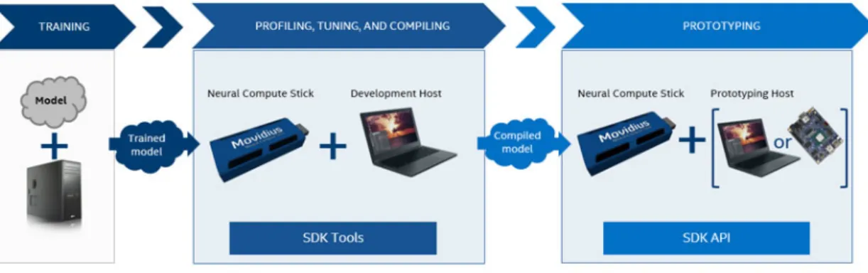
The Intel Movidius Neural Compute Stick (NCS) [18] is a USB fanless device for deploying deep learning applications at the edge without the usage of cloud-based services. The NCS is powered by low power high performance Intel Movidius VPU that is widely used in smart security cameras, drones or industrial machine vision equipment. The VPU uses 12 processors to accelerate computing by running parts of the networks in parallel. The NCS is used with Intel Movidius Neural Compute SDK that allows to profile, tune, and deploy DNNs on low-power devices that require real-time inferencing3. DNNs are trained using host machine and transfered to the NCS in a special graph representation via Neural Compute API (NCAPI). A graph network is attached to the VPU by NCAPI and is ready to be queried by the user. The output of the network is sent to the user via the USB connection and received by the application with NCAPI. What the output represents (labels or probabilities) is configured during a network graph generation and can only be changed by generating a new network graph.
Figure 4: Intel Movidius NCS workflow
The NCS typical workflow example4 is shown in Figure4.
3https://developer.movidius.com/
3
Problem Statement
3.1
Threat Model
The threat model of extraction attacks is described in this section. It consists of three parts: the attack surface, the attacker’s capabilities and the attacker’s goals. Attack surface. An attacker can target any prediction API that responds with labels or probabilities to a given input. In this thesis we consider two following API scenarios:
Cloud-based prediction API. A malicious user interacts with a MLaaS platform, models protected by local isolation using trusted execution environment [34, 11] or by encrypted prediction schemes [27]. Systems themself are placed in a secure environment (e.g. cloud, network) and direct access to internal parts of the system are not allowed. The basic requirement of the attack is to have access to outputs of a target machine learning models. The attack is limited to neural networks. A simplistic scheme can be found in Figure5.
Input data
Labels/probabilities
Attacker
MLaaS
Figure 5: Scheme of cloud-based attack scenario
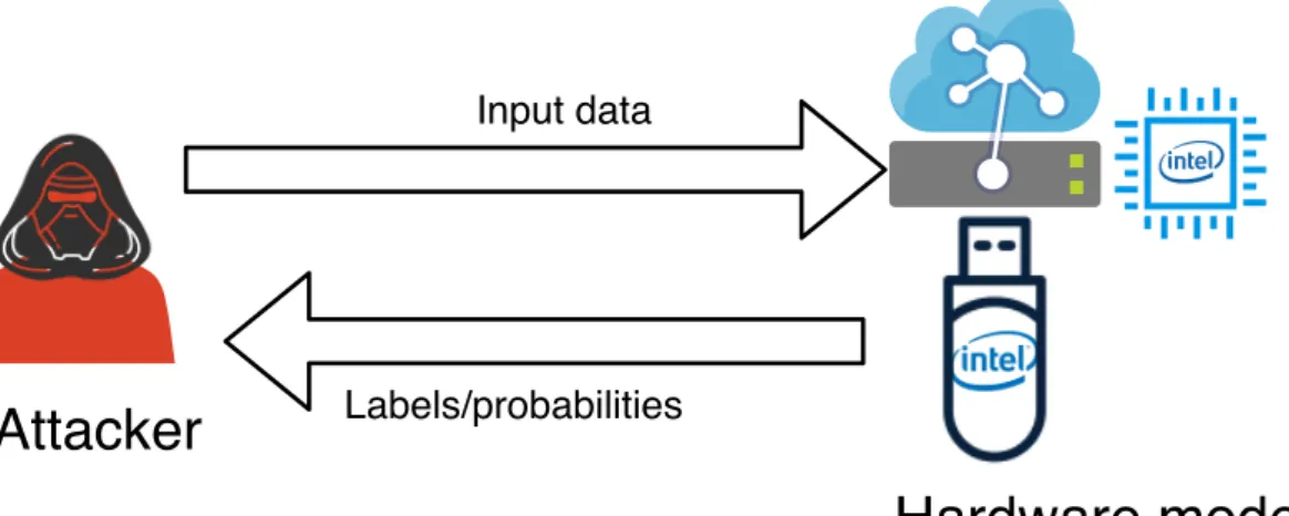
Hardware-supported prediction API.In this scenario, a model is embedded in some device. The server could have hardware-based protection, such as a TEE, e.g. Intel-SGX [39]. The model is intended to be used in real time, therefore, an attacker has several options to get predictions.
1. An adversary obtains a device if it is publicly available, for instance, an autonomous driving vehicle where the model should be provided, and tries to extract the model locally. Therefore, this scenario converges to the original attack described in the previous section. An adversary then could find suitable
adversarial examples and would theoretically have no limit on time. We evaluate this scenario in Section 6.3.
2. When no access to an API can be obtained, an attacker can still have physical access to the input sensor and can feed arbitrary data. Supposedly, an adversary would be able to send input as either physical printed images by showing it in front of the camera or by putting a screen in front where images would appear with a certain time gap. Undoubtedly, an attacker also would need to get access to decisions of the model somehow. This scenario is less plausible.
In Figure 6we present a simple scheme of attack scenario on dedicated hardware prediction API.
Input data
Labels/probabilities
Attacker
Hardware model
Figure 6: Scheme of hardware-based attack scenario
Attacker’s capabilities. An adversary (Attacker) is assumed to have black-box access to the model (only access to prediction API). Attacker knows the nature of the input (classification task), shape of the input and output layers of the model. Attacker can send queries to the server and get probabilities or labels (or both) as a response. We assume that Attacker knows the model architecture, but not the parameters. He has no access to model internal data and processes as well as to the training data. The classes are presumed to be meaningful and correspond to a particular object of classification, i.e images, diseases etc. Attacker has access to a DNN training environment with commodity hardware. He is not limited in time, but in the number of queries he sends to the model.
Those assumptions are similar to the ones made in [36] and the main assumption is that Attacker should have access to some initial data from the same or similar
distribution targets as training data came from. However, assumptions made in this thesis are different from [27], which assumed that a malicious user has no intuition about its classification task, about what the input must look like, but rather only the shape of input and its domain.
Attacker’s goals. The main objective of Attacker is to train a new model (attacker model) which closely resembles the target model based on classification performance on an unseen test set. Attacker has a budget limit and wishes to spend it as effectively as possible to "steal" the target model. The number of queries and their nature can be tracked by MLaaS service provider or any third-party service that is responsible for server maintenance. The secondary goal of Attacker is to create transferable adversarial examples, i.e to find perturbationϵ for an input x of class c such that
x+ϵ is classified as c′ ̸= c by target model F. In other words Attacker selects a target classc′ and uses algorithm from Section 2.5.1 to create new images x+ϵfrom original images that are classified as c′
F(x+ϵ) =F′(x+ϵ) =c′ (16) The perturbation size ϵ is bounded.
Therefore, Attacker tries to retain image appearance to be almost unnoticeable for the human eye. In contrast to previous work, we require that the attacker should be able to create targeted adversarial examples, i.e. misclassification into specific classes.
3.2
Requirements
The primary goal of this thesis is to critically evaluate existing model extraction techniques and to develop new techniques to extract a model from MLaaS platforms. The intended solution should be able to outperform existing attacks [36,41]. There-fore, in the furtherance of the work done in this thesis, the solutions must fulfill the following requirements:
Implementation requirements
The implementation requirements serve as a basis for design decisions on the repro-duction of existing attacks and developing new techniques using Python Pytorch library [37] that is rapidly developing and widely used in the ML community.
I1 Implementation of any method in this work must be done using Pytorch library from Python.
Performance requirements
The performance requirements are parts of improving on existing attacks. We state the following desiderata to evaluate this thesis in comparison with previous work. The quality of the solution is evaluated with regards to the following metrics.
P1 F-agreement In order for the attack to be considered successful an algorithm must produce a close approximation of target model. We aim to reach up to
∼20 % performance improvement compared to previous attacks.
P2 Transferability rate Another attack performance metric is how good the ex-tracted model for crafting targeted transferable adversarial examples. We aim to reach up to ∼20 % performance improvement comparing to previous attacks.
P3 Budget limit The attacker has a budget limit and our technique must fulfill requirements P1 and P2 using fewer queries than state-of-the-art [41, 36].
P4 Reliance of natural initial samples. The proposed solution should rely on a few natural initial samples. Higher F-agreement and Transferability rate should be achieved using less initial samples compared to Papernot attack [36].
Scalability requirements
Our scalability requirements refer to the ability of the solution to be used in a range of applications. We evaluate attacks on dedicated hardware (Intel Movidius Neural Compute stick)
S1 Create an interface to communicate with Intel Movidius Neural Compute stick using the same implementation in Pytorch that corresponds to Performance requirements P1 to P4.
4
Methodology
The previous section identified the problem scope of attacks against DNNs and discussed main threats that can arise due to a malicious behaviour. In addition, we identified the requirements for designing new techniques. Therefore, in this section we describe how we reproduced existing work on model extraction attacks. We also give an overview of new techniques to extract a ML model from a cloud service or locally deployed that fulfills these requirements.
Previous work in model extraction that is used in this work as a baseline is done by Papernot et al. and Tramer et al. [36, 41]. Tramer et al. evaluated the attack only using "toy" low-dimensional data and evaluating efficiency only based on the number of queries sent to the server. Papernot et al. expanded the attack to use more realistic images. However, the only parameter in the attack that Papernot et al. reported in evaluation is perturbationϵused in FGSM to generate synthetic data. In this work we identify and evaluate parameters in model extraction attacks that can improve extraction performance and catalyze the attack, such as different learning strategies (Section 4.1) and the amount of initial data the attacker has access to (Section 6.2.1).
We propose several novel techniques to query the target model. In general all approaches follow the same trend, which is crafting new synthetic data by querying the target model in some areas of interest. This may be going in the direction of the specifically chosen class or to opposite direction of the original class as in a previous solution [35].
The general scheme to extract DNN models can be systematized into the follow-ingListing 1. We assume the target DNN classifierF and the attacker modelF′ that mimicsF. Hyperparameters ofF, such as the number of layers, the number of hidden neurons and activation functions are assumed to be known. These could be partially obtained using techniques from [33, 42]. We train F′ using a minimum number of labeled training samples, as defined by a maximum prediction query budgetb toF.
Model extraction algorithm can be described in the following way:
Listing 1: Steps in model extraction attacks.
1. Choosing model hyperparameters. Attacker selects a model architecture and hyperparameters to use for training his local model F′.
2. Initial sample selection.Attacker collects an initial set of unlabeled samples that build the foundation to catalyze the extraction attack, i.e. the attacker set. Samples are chosen depending on the the nature of the model input data (e.g. traffic signs or digit classification), and knowledge of what the output
classes of the model mean (e.g. stop signs or number "9").
Duplication round
3. Querying target model for prediction. Unlabeled samples are sent to the target model in order to obtain labels/probabilities for them. These new labeled data are used as ordinary labeled data in next steps.
4. Training local attacker model. All labeled samples are used as a training set for the attacker model using a defined training strategy. We perform the intermediate evaluation of the attacker model after this step.
5. Synthetic sample generation.The method of generating new samples differs per technique. We use Jacobian-based sample generation technique to explore the input space in important areas. It is based on techniques for creating adversarial examples (Section 2.5.1). Newly generated data is then augmented to a dataset and used in step 3.
Steps 3 to 5 are looped until reaching some stopping criteria. It can either be until reaching adequate F-agreement value (P1) or until budget (P2) limit is reached.
4.1
Attacker model learning strategies
Previous work has not evaluated the impact of the learning strategy used by the attacker. The DNN background that is used in this thesis are described in Section2.3, CNN in particular. CNNs requires several learning parameters optimized to achieve the best performance not only in training the model but also in the attack. Here we try to describe such parameters and give a general overview of their role in the attack.
Learning rate is the parameter used in gradient-based training to control the speed of learning on each iteration. It is well-known to be crucial in training of the model [23], and naturally will impact the model extraction attack (Section 4),
as it requires several rounds of training. The learning rate value also depends on regularization techniques used in training. Therefore, in this work we use a 5 fold cross validation scheme to estimate the right value for learning rate in different scenarios.
Regularization is usually used in training to avoid over-fitting and achieve better generalization of decision boundaries. It can be applied in training of the attacker model in several ways, such as L1 or L2-penalty and/or dropout (see Section2.2.1). We found that the impact of L1 or L2 regularization penalty was small, but dropout tended to boost certain aspects of the attack.
Transfer learning relates to re-using machine-stored knowledge that was gained during previous training to solve the particular task and assign this knowledge to another related problem. One of the techniques that is used in transfer learning is to stop updating certain layers during back-propagation. This is called layer freezing [10, 26]. Therefore, during our first duplication round phase (Listing 1) model trained for one round might already have enough knowledge in intermediate convolutional layers such that it does not need further training. The benefit of layer freezing is faster training [10, 26]. CNNs convolutional layers tend to show poor ability to expand knowledge by taking new data bit by bit and, therefore we propose to "freeze" (stop updating them during backpropagation) all convolutional layers after first round of training on initial attacker set is done and for following duplication rounds we update only fully-connected (dense) last layers of the network, such as non-convolutional ReLU and Softmax layers (described in Section2.2.2).
Model re-initialization In general, synthetic data generation technique can be described as incremental learning [19] as we feed more and more data to the model and re-train a classifier incrementally with the new data. CNNs tend to show poor performance in learning when new data introduced gradually over time and require the use of separate techniques to improve learning quality, such as feature extraction, fine-tuning, learning without forgetting [26]. Another problem in CNNs is the so-called "dying ReLU" problem [4]. ReLU outputs always zero when the input is negative therefore if during back-propagation part of the inputs become negative then those neurons are likely to be "dead" and have no effect in training. Sigmoid and Tanh activation functions can experience the same problems as their values
saturate. However, one solution to "dying ReLU" is to either use Leaky-ReLU or PReLU [15]. Both of these help only in long term and require a large set of data to "recover" a "dead" neuron in order to start learning again. Re-initializing all "dead"
neurons with random values and allowing them to update normally according to gradient optimization algorithm used is highly time and power consuming. Thus, we propose a method to avoid the "dead" neurons and possibly improve learning experience by re-initializating model after each duplication round and train it from scratch, incrementally adding new synthetic data.
4.2
Synthetic sample generation
We use the attacker set, a subset of original data or data from the same distribution, to generate synthetic samples from labeled data. The goal is to increase the training set for the local classifier in order to better extract the target DNN model. Synthetic data generation is done in a way to explore target model’s decision boundaries and get a better understanding of the classifier. We use the Jacobian matrix in accordance with the local classifier and update the model at each duplication round to improve the quality of crafted samples. To achieve better F-agreement with original classifier we explore the space in some directions of interest that we choose according to some specific query strategy. New synthetic samples are generated either with Fast Gradient Sign Method (FGSM) [13] or Projected Gradient Descent (PGD) [30], described in Section2.5.1. We evaluated new approaches to find a suitable target label to craft synthetic data from the original set.
4.2.1 Jb-star approach
The idea in this approach is to query all possible target labels from a given classc, i.em−1 directions, wherem is the number of classes. By doing so we explore all possible decision boundaries of each class and expand the attacker model knowledge by querying all directions. The problem with this approach is that the synthetic data grows exponentially by factorm. Therefore, it takes a lot of time and resources to explore all directions. For instance, we retrain forN duplication rounds, therefore the total number of crafted samples would be D0 ×(m)N where D0 is the size of
the attacker set that we start with. Even with simple multi-label classification task we need to store and send to the target model an enormous number of samples. Therefore, we decided to simplify this approach by exploring only some directions
further on.
4.2.2 Jb-Top-k approach
This approach is based on selecting target labels that are the closest to a given sample according to softmax probabilities from attacker’s classifier. The reason behind selecting spatially closest classes is to attempt to get a better approximation of target classifier’s decision boundaries. Consequently, selecting only the "best" target labels would save time and resources considering that exploring all directions would be too expensive.
The algorithm to find spatially closest targets to a sample xis following:
1. calculate probability distribution of the samplex which isp1..m w.r.t all classes [1..m] using an attacker model
2. exclude the original class probability and sort the remaining probabilities from highest to lowest
3. afterwards, select the top-k classes and create synthetic samples with respect to these
Overall, as it was previously stated the amount of synthetic data will exponentially increase throughout duplication rounds by a factor ofk+1. Therefore in our evaluation (Section6) we choosek up to 3 in case of GTSRB andk up to 7 in MNIST, restricting the number of duplication rounds as well to keep the total number of queries within an acceptable range.
The top-k approach can be described using following equation:
x′c′ =x+ϵ, s.t. ϵ= arg max
ϵ
F′(x+ϵ)[c′], c′ ̸=F′(x) (17) where c and c′ are the original and target label correspondingly; F′ is the local attacker model andF′(x) is the class prediction from it; ϵ is a perturbation to the target class direction derived from attacker model using the Jacobian matrix and one of the techniques described in Section 2.5.1.
Consequently, in each duplication round the attacker set is augmented with new samples that the attacker model F′ is likely to misclassify thus exploring areas of the input space that the model is the least certain about.
4.2.3 Jb-self approach
The concept of this technique is to apply methods from Section 2.5.1 using the same original label as the target. In consequence, it tries to give a better understanding of where part of original data lies, i.e. the most representative point of the class. It is done in accordance with the fact that the best way to reproduce original model’s decision boundary is to train on the same data that the model was trained on.
Therefore, Jb-self can be viewed as the following formula:
x′c=x+ϵ, s.t. ϵ = arg max ϵ
F′(x+ϵ)[c], c=F′(x) (18) where c and c′ are the original and target label correspondingly; F′ is the local attacker model;ϵ is a perturbation to the original (self) class direction derived from the attacker model using Jacobian matrix and one of the techniques described in Section2.5.1.
4.3
Evaluation of model extraction
We evaluate the success of the attack using F-agreement and transferability rate.
4.3.1 F-agreement
F-agreement (see Section2.2.3) is calculated with respect to the target model predic-tions as the ground truth data and the attacker model predicpredic-tions as the held out data. We compare a number of predictions that models agree on to the total number of labels in data. It shows how well the attacker model agrees with the target model even though datasets may be imbalanced. We choose F-score agreement rather than prediction accuracy mainly to get a fair comparison of models and deal with class imbalance if any.
4.3.2 Transferability rate
Transferability was introduced by [24] (Section 2.6.2). We use a ratio of transferable examples to the total number of created adversarial examples as a performance metric called transferability rate. According to previous work (Section2.6) transferability rate grows if the F-agreement between an attacker model and a target model increases. Adversarial examples can be targeted and untargeted. Targeted adversarial example refers to a sample that is crafted to be some specific (target) class that is different
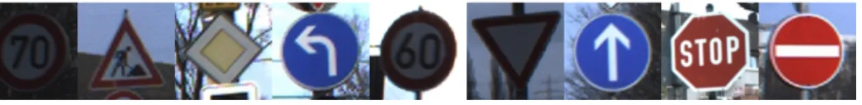
from the original. Untargeted corresponds to a sample that is meant to be any other class but the original. The choice of which transferability rate is more appropriate to a certain case strongly depends on attacker’s motivation and goals. Untargeted transferability may be enough to lower the overall prediction quality since it is faster to generate and requires less exactness in the attacker model in comparison with the target model. In another case, the attacker’s goal may be to change all "Stop signs" to "Speed limits" or "Go straight" sign in this case targeted transferability is the appropriate choice for the attacker. In this thesis, we evaluate targeted transferability rate. We use an attacker set of initial samples to measure transferability rate. In case of MNIST, we target each sample to all other classes. In GTSRB there are too many classes to evaluate (42 directions to craft) so we propose a certain scheme to evaluate targeted transferability rate (see Section5.2) by grouping several similar classes to a new macro-class and use it as a target. All of these attacks are also possible in a white-box environment where an attacker has access to a target model internal outputs, such as loss and back-propagation. In white-box scenario targeted and untargeted transferability rates are expected to be much higher.
5
Datasets and experimental setups
In the previous section, we described the methodology of our approach in general. This section presents an overview of datasets that are used throughout experiments and evaluation. Moreover, we describe two experimental setups used in this work.
For evaluation of proposed techniques in Section 4 and state-of-the-art tech-niques [35, 41] two main datasets are used in this work: MNIST and GTSRB. A brief overview of each dataset is presented below.
5.1
Mixed National Institute of Standards and Technology
(MNIST)
MNIST dataset consists of 28×28 handwritten digits. It contains 10 classes (from 0 to 9). It is a subset of a larger set from NIST. All images were rescaled to fit in 20×20 boxes preserving their properties, centered and normalized to be gray-scale. MNIST dataset is constructed from NIST’s Special Database 3 and Special Database 1. Special databases in NIST contain images of handwritten digits from different people. For example, SD-3 was accumulated from Census Bureau employees, whereas SD-1 was collected in a group of students. The resulting MNIST training set is built from 30,000 images from SD-3 and 30,000 images from SD-1. The test set consists of 5,000 images from SD-3 and 5,000 images from SD-1. Overall, the dataset is composed of images that were written by ∼ 250 distinct writers. Test set and training set are composed from different writers.
• Training set contains 60,000 images
• Test set - 10,000
Example inputs from each of the 10 classes from MNIST that vary within the same class are shown in Figure7.
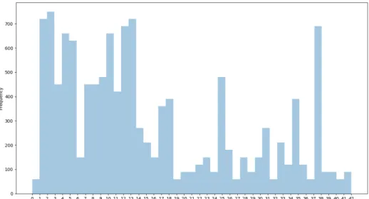
The number of images in each class in the test set is shown in Figure8. Since the dataset is balanced, it is easy to reserve an equally divided set of samples from original data and use it as attacker set. Therefore, we reserve 5,000 (500 from each class) images from the training set, which are not used later on in training the target model. This dataset (or a subset of it) is used as the attacker set in our experiments with MNIST.
Figure 7: Example images from MNIST.
Figure 8: Distribution of classes in MNIST test set.
![Figure 2: An illustration of adversarial image using FGSM [13].](https://thumb-us.123doks.com/thumbv2/123dok_us/9021838.2800034/22.892.156.755.299.539/figure-illustration-adversarial-image-using-fgsm.webp)
![Figure 3: An illustration of an adversarial image using PGD method [30].](https://thumb-us.123doks.com/thumbv2/123dok_us/9021838.2800034/23.892.151.736.303.543/figure-illustration-adversarial-image-using-pgd-method.webp)