Edge-Computing Deep Learning-Based Computer Vision Systems

(1)

Clemson University

TigerPrints

All Dissertations

Dissertations

12-2018

Edge-Computing Deep Learning-Based Computer

Vision Systems

Edwin Lee Weill

Clemson University, eweill@g.clemson.edu

Follow this and additional works at:

https://tigerprints.clemson.edu/all_dissertations

This Dissertation is brought to you for free and open access by the Dissertations at TigerPrints. It has been accepted for inclusion in All Dissertations by an authorized administrator of TigerPrints. For more information, please contactkokeefe@clemson.edu.

Recommended Citation

Weill, Edwin Lee, "Edge-Computing Deep Learning-Based Computer Vision Systems" (2018).All Dissertations. 2285.

(2)

Edge-Computing Deep Learning-based

Computer Vision Systems

A Dissertation Presented to the Graduate School of

Clemson University

In Partial Fulfillment of the Requirements for the Degree

Doctor of Philosophy Computer Engineering by EdwinWeill December 2018 Accepted by:

Dr. Melissa Smith, Committee Chair Dr. Robert J. Schalkoff

Dr. Harlan Russell Dr. Amy Apon

(3)

Abstract

Computer vision has become ubiquitous in today’s society, with applications ranging from

medical imaging to visual diagnostics to aerial monitoring to self-driving vehicles and many more.

Common to many of these applications are visual perception systems which consist of classification,

localization, detection, and segmentation components, just to name a few. Recently, the

develop-ment of deep neural networks (DNN) have led to great advancedevelop-ments in pushing state-of-the-art

performance in each of these areas. Unlike traditional computer vision algorithms, DNNs have the

ability to generalize features previously hand-crafted by engineers specific to the application; this

assumption models the human visual system’s ability to generalize its surroundings. Moreover,

con-volutional neural networks (CNN) have been shown to not only match, but exceed performance of

traditional computer vision algorithms as the filters of the network are able to learn "important"

features present in the data.

In this research we aim to develop numerous applications including visual warehouse

diag-nostics and shipping yard managements systems, aerial monitoring and tracking from the perspective

of the drone, perception system model for an autonomous vehicle, and vehicle re-identification for

surveillance and security. The deep learning models developed for each application attempt to match

or exceed state-of-the-art performance in both accuracy and inference time; however, this is

typi-cally a trade-off when designing a network where one or the other can be maximized. We investigate

numerous object-detection architectures including Faster R-CNN [1, 2], SSD [3], YOLO [4, 5], and

a few other variations in an attempt to determine the best architecture for each application. We

constrain performance metrics to only investigate inference times rather than training times as none

of the optimizations performed in this research have any effect on training time. Further, we will

also investigate re-identification of vehicles as a separate application add-on to the object-detection

(4)

techniques for security and surveillance.

We also investigate comparisons between architectures that could possibly lead to the

devel-opment of new architectures with the ability to not only perform inference relatively quickly (or in

close-to real-time), but also match the state-of-the-art in accuracy performance. New architecture

development, however, depends on the application and its requirements; some applications need to

run on edge-computing (EC) devices, while others have slightly larger inference windows which allow

(5)

Dedication

This dissertation is dedicated to my academic advisor without whose constant support and

guidance this research would not have been possible. This dissertation is also dedicated to my wife,

parents, and sister, who have always been supportive and an inspiration to pursue interests and

(6)

Acknowledgments

This dissertation was made possible by the tremendous help and support of the following

faculty members, family members, and colleagues.

I begin by thanking my academic advisor, Dr. Melissa C. Smith, who graciously accepted

me as her pupil. Dr. Smith’s words of wisdom, immense experience, constant encouragement,

insightful suggestions, and limitless networking ability allowed for the completion of this research

and dissertation.

Secondly, I would like to thank Dr. Robert Schalkoff for his support through the entire

doctoral process as well as the instruction he has provided as a professor and mentor. His immense

knowledge in the fields of machine learning and artificial intelligence have not only aided me in my

studies and research but his enjoyment of the field has motivated me to pursue this topic in a way

that would not be possible without constant stimulation.

I would also like to thank Dr. Amy Apon and Dr. Harlan Russell for serving on my doctoral

committee and instructing me in various fields of computer architecture, computer vision, and high

performance computing.

I am also thankful for my wife, Hiliary, my parents, Edwin and Jeanine, and my sister,

Shannon, who provided constant support during the research process and writing of this manuscript.

I also owe a debt of gratitude to my fellow colleagues from the Future Computing

Tech-nologies Laboratory (FCTL) at Clemson University: Jesse, Varun, Ankit, Jamar, Karan, and many

others whom I fail to mention for providing me a stimulating work environment during this process.

I also owe thanks to Ashraf and Vivek (previous Ph.D. students of Dr. Smith’s FCTL) without

whom I may not have pursued graduate school. A special thanks goes to Jesse for assisting greatly

in helping get our current research to a phase where growth was imminent after this document has

(7)

I would also like to mention a few members of my team at NVIDIA (Ratnesh, Arihant,

and Varun) with whom I discussed many of the ideas presented in this thesis (especially the topics

involving re-identification) as well as submitted a paper and patent to go along with the work.

Lastly, I would like to acknowledge the Engineering and Science Education department at

Clemson University for providing the Graduate Assistants in Areas of National Need (GAANN)

Fellowship. This fellowship has provided learning experiences in not only education research but in

correct teaching practices and methods. I would also like to acknowledge André Luckow at BMW for

providing funding for computing hardware as well as travel expenses for attending top-tier computing

conference, without which I would not have been able to see first hand the research being performed

(8)

List of Tables

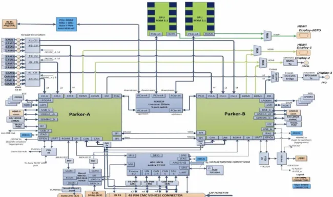
3.1 NVIDIA Drive PX2 Specifications . . . 38

3.2 Titan X Inference Times . . . 44

3.3 NVIDIA Jetson TX2 Specifications . . . 45

4.1 Faster-RCNN Inference Times . . . 64

4.2 TensorRT Classification Model Optimizations on Jetson AGX Xavier (time in ms) . 81 4.3 TensorRT Detection Model Optimizations on Jetson AGX Xavier (time in ms) . . . 82

(11)

List of Figures

2.1 AI Overview . . . 5

2.2 Single Neuron . . . 7

2.3 Activation Functions . . . 8

2.4 Shallow Feed Forward Network Architecture . . . 9

2.5 Multi-layer perceptron . . . 10 2.6 Convolution [6] . . . 14 2.7 Convolution Filters [7] . . . 15 2.8 Receptive Field [8] . . . 16 2.9 Image Classification . . . 18 2.10 AlexNet Architecture . . . 19 2.11 VGG Architecture . . . 20 2.12 GoogleNet Architecture . . . 20 2.13 ResNet Unit . . . 21 2.14 Faster RCNN Architecture . . . 24 2.15 YOLO Example . . . 25 2.16 SSD Architecture . . . 25

2.17 Samples from VeRi [9] Dataset (Each Row is Seperate Identity) . . . 27

2.18 Re-Identification Process for Creating Embeddings for Objects . . . 29

2.19 Vehicle Re-Identification Datasets . . . 29

2.20 Triplet Loss Optimization . . . 31

3.1 Autonomous Driving Architecture . . . 36

3.2 NVIDIA Drive PX2 Architecture . . . 38

3.3 Perception Module . . . 39

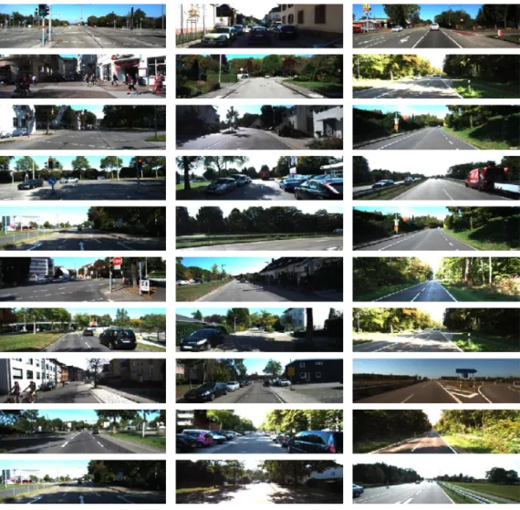
3.4 Example Images from the KITTI dataset . . . 40

3.5 Example Images from the LISA dataset . . . 40

3.6 DetectNet Architecture [10] . . . 41

3.7 DetectNet Inference Architecture [10] . . . 42

3.8 DetectNet-Depth Architecture . . . 42

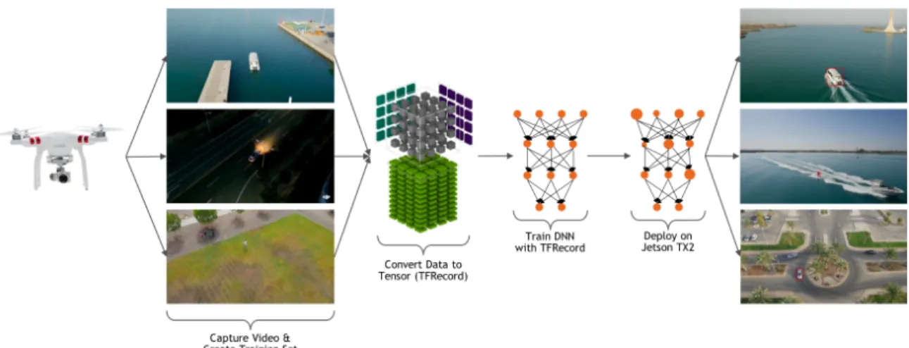
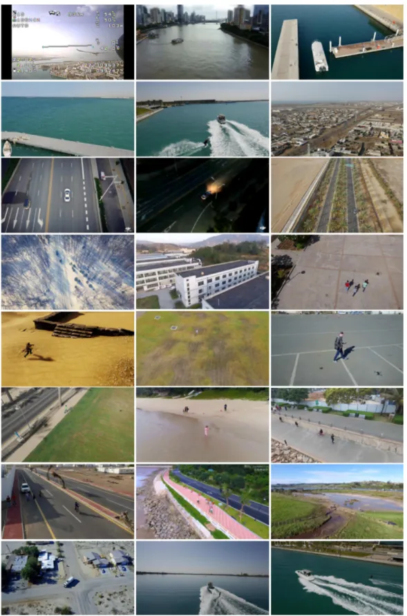
3.9 DAC Pipeline . . . 45

3.10 DAC Dataset Samples . . . 46

3.11 Embedded SSD (eSSD) Architecture . . . 48

3.12 Barcode Label Synthetic Dataset Samples . . . 51

3.13 Barcode Label Detection Pipeline . . . 52

3.14 YOLO Architecture . . . 53

3.15 Tiny-YOLO Architecture . . . 54

3.16 Trailer ID/Parking Lot Detection Pipeline . . . 54

3.17 Trailer ID/Parking ID Dataset Samples . . . 55

3.18 Batch Data Selection Techniques . . . 59

(12)

4.2 Gallery Image Ranking Based onProbe Image . . . 63

4.3 Faster-RCNN Vehicle/Pedestrian Detection . . . 64

4.4 Example 1: DetectNet Depth Image . . . 65

4.5 Example 2: DetectNet Depth Image . . . 66

4.6 Jetson TX2 Inference Times on KITTI Images . . . 67

4.7 KITTI Statistics [11] . . . 67

4.8 Inference on KITTI Cars . . . 67

4.9 Inference on KITTI Pedestrians . . . 68

4.10 DAC mAP Results . . . 69

4.11 Evaluation Results of eSSD Architecture . . . 71

4.12 DAC Challenge Output 1 . . . 71

4.13 DAC Challenge Output 2 . . . 72

4.14 Barcode Label Detection Performance . . . 73

4.15 Synthetic Inference . . . 73

4.16 Real Warehouse Barcode Detection . . . 73

4.17 iPhone 7 Plus Label Detection Inference . . . 74

4.18 Trailer ID/Parking Number Detection Performance . . . 75

4.19 Trailer ID Detection and Preliminary OCR . . . 76

4.20 Visual Results for Vehicle Re-Identification with VeRi Dataset. Green are Correct Retrievals whileRedare Incorrect Retrievals (All from Different Cameras) . . . 79

(13)

Nomenclature

AD Autonomous Driving

ADAS Advanced Driver Assistant Systems

AN N Artificial Neural Networks

CN N Convolutional Neural Network

DL Deep Learning

DN N Deep Neural Network

EC Edge Computing

eSSD Embedded Single-Shot Multi-box Detector

F P S Frames Per Second

IoU Intersection over Union

mAP Mean Average Precision

M LP Multi-layer Perceptron

ReLU Rectified Linear Unit

RP N Region Proposal Network

SSE Sum of Squared Errors

(14)

Chapter 1 Introduction

In recent years, deep learning has become one of the largest contenders in many different

fields of research. In particular, fields such as computer vision, robotics, and natural language

processing have been effected greatly. With the success of deep learning architecture like CNNs,

developers now have the ability to no longer hand craft features or algorithms for their specialized

applications. Deep learning has shown itself to be efficacious in learning abstract patterns in data

rather than hand-designing them for a specific application. DNNs (in particular CNNs) have become

the state-of-the-art in their ability to not only learn representations of the data but also construct

features at many scales, orientations, etc. from a trainable dataset. An algorithm that has the

ability to learn on its own rather than be instructed through the learning process has been the

impetus for the growth of deep learning in a wide range of applications. Through extraction of

features enumerated in the learned weights of a DNN, they are able to compete with (if not exceed)

the accuracy and speed of traditional computer vision tasks with the added advantage of not having

to hand-craft algorithmic-specific and data-specific features.

Many of the cutting-edge breakthroughs that have occurred in recent years have been either

optimizing the training and inference process, novel frameworks and architectures, or using and

existing architecture to tackle a real-world application or problem (the focus of most of this research).

Some of the heaviest players in the field of deep learning are start-ups, companies, and university

teams focusing on automation and autonomous systems. For example self-driving cars or self-flying

drones are defined by their ability to act on demand rather than having a human control them.

(15)

providing useful information to the subsystems which control the motion and other components.

Even though these systems attempt to use cutting-edge technology, they are often hindered by the

safety constraints imposed on them by obstacles in the environment. For this reason, systems that

are deployed on mobile robots like drones or self-driving cars must not only go through rigorous

testing but also be able to execute in real-time to combat issues that may occur in the environment.

When comparing all autonomous systems, to some degree, they all utilize the same

technol-ogy for motion in an environment. First, there must be some subsystem which can reason about the

objects or important artifacts of an environment and then decisions must be made based on these

artifacts. For autonomous driving, some of these artifacts could include location of all vehicles and

pedestrians in the local vicinity as well as information about the road itself including lane markings,

turns, etc. The main object of any supervised autonomous system is to retrieve some information

from its sensors, extract and process information about the scene, and the pass along that

informa-tion to a planning module which can make decisions about proposed path and speed for the system.

Due to the complexity of these systems, developers look for every portion which can be accelerated

or re-factored in an effort to learn a better representation of its environment while also making it as

efficient and fast as possible.

In this work, we set out to tackle four different tasks: autonomous driving, drone surveillance

detection, warehouse management systems, and vehicle re-identification. With each of these tasks,

we will be working towards a real-time solution (being able to run inference on models in real-time).

In collaboration with CUICAR, we have developed a perception module for autonomous driving

with the ability to not only estimate the position of important objects in the scene such as vehicles,

pedestrians, and signs but also estimate their distance from the camera (or autonomous system

mounted camera). We have also developed an inference engine with the ability to detect objects in a

drone-vision (aerial) setting including vehicles, pedestrians, boats, and many more objects. Further,

we have developed a two DNN-based system for BMW: one for localizing and scanning barcodes

on shipping labels and a second for detecting trailers in a train yard as well as the parking spots

in which they are currently located. Lastly, we have developed a solution for identifying vehicles

within a multi-camera system without the need for camera-to-camera tracking; rather establishing

a signature for each of the vehicles.

The remainder of this dissertation is organized as follows. Chapter 2 provides background

(16)

Also, throughout Chapter 2, we have described some of the relevant literature that has been

devel-oped in fields like CNNs, deep learning, object detection, and re-identification. The combination

of background and literature review amalgamate to provide the motivating force for designing the

numerous applications in this dissertation. Chapter 3 presents each of the applications as well as

the overall system design and DNN architecture designs (and trade-offs) specific to each application.

Also Chapter 3 enumerates the experiments that were completed with developing each application.

We wrap up this dissertation with Chapter 4 presenting the results for each application and

experiments as well as conclusions for each. Chapter 5 concludes by enumerating the contributions

that this work has provided (including best practices for creating an edge computing system) as well

(17)

Chapter 2 Background & Literature Review

In this chapter, basic machine learning and computer vision concepts will be discussed as

an introduction to the applications to be discussed as part of the work provided for this dissertation.

First, we will discuss machine learning basics including machine learning algorithms, neural networks,

deep learning and optimization techniques for these algorithms (i.e. "training"). Next, we will

discuss traditional computer vision and how it has played a role in recent history in the birth

of deep learning and feature extraction networks. In this section we will also discuss traditional

architectures for each of the computer vision-based deep learning techniques. Finally, we will discuss

the concept of metric or representation learning, which will allow for a discussion of triplet loss and

the re-identification problem.

2.1 Machine Learning

In this section, we will discuss machine learning basics as well as provide more in-depth

discussions of both traditional neural networks and their evolution into deep neural network models.

A discussion of deep learning frameworks as well as how to utilize them for training and inference

are also discussed in this section.

2.1.1 Machine Learning Basics

Machine learning (often interchanged with the terms artificial intelligence and deep learning)

(18)

(a) AI Venn Diagram

(b) AI Flow Chart

Figure 2.1: AI Overview

intelligence is typically used for a much broader concept of machines that have the ability to carry

out tasks in a manner by which they are considered "intelligent". Machine learning, on the other

hand, is built around the idea that providing a machine with a certain amount of data, it should be

able to learn something meaningful on its own. Goodfellow, et al. [13] illustrate this through a very

helpful diagram and flowchart, shown in Figure 2.1.

As the Venn diagram alludes to, deep learning can be thought of as a type of representation

learning, which is a type of machine learning. Following this, machine learning is shown as a subset

of AI; however, it should be mentioned that not all AI approaches utilize machine learning as a

solution. Machine learning can be thought of as a system that is provided some sort of data D, placed in some "environment"E, is designed for a specific set of tasksT and is evaluated on some performance metric P. A mathematical interpretation of this is shown below as an optimization problem.

maximize

D P(D)

subject to Ti(D)⊂E, i= 1, . . . , m.

(2.1)

(19)

to maximize the performance metric,P, given some dataD by training onmtasksTicontained in the

training environmentE. For example, we may be asked to train a clustering algorithm to determine the differences in certain types of clothing (i.e., shirts, shorts, jeans, shoes, etc.). Our clustering

algorithm (machine learning algorithm) will take as input a set of data D which is representative of the data we would like to cluster. We will then perform distance calculations and mean updates

(tasks Ti) inside the environment (i.e group of data for clustering) that will group all like objects

together. The performance metric we will be maximizing is the number of correct examples that are

placed in each group after training (assuming we have labeled data).

When compared to traditional algorithms, machine learning is able to aide developers and

scientists in creating easier solutions to higher dimensional problems which before needed hand

crafted algorithms developed by experts in the field. As can be seen in the Venn diagram in Figure

2.1a, logistic regression is a perfect example of a traditional machine learning algorithm. Logistic

regression is involves solving for some output y given some set of inputsx and which are linearly combined with equation coefficients (later called weights in neural networks) forming the equation

y =wT_x_where _y _{is the output,} _x _{is the input, and}_w _{are the equation coefficients. Later we will}

discuss thewterms as the weights of a neural network rather than coefficients of an equation. Figure 2.1b illustrates that for classical machine learning techniques, there are hand-designed features that

are used for converting the inputs to features which the machine learning algorithm can use.

A subset of machine learning is representation learning. In representation learning, we have

removed the dependency on hand-crafted features by the designer and allow the algorithm (network

or other) to develop its own interpretation of the data, in turn developing its own set of features.

This can be seen in the second from right column of the flow chart in Figure 2.1b. An example of this

would be a simple neural network which will be discussed in the next section in more detail. However,

in short, the neural network is able to use the data provided to create a "representation" of the data

(normally in a smaller dimensionality than the original data). The goal of representation learning

is to allow the system to learn representations of the data rather than the scientist or developer

hand-crafting each feature; most of the time, this yields to much higher performance. Numerous

algorithms including neural networks, deep learning, and numerous unsupervised techniques utilize

the idea of representation learning to learn from a large set of data.

In the next section, we will go more in depth into artificial neural networks and how they

(20)

Figure 2.2: Single Neuron

2.1.2 Neural Networks

An Artificial Neural Networks (ANN) is a computational model which is slightly modeled

by the way biological neural networks in the human brain process information. With that said,

ANNs (at least those designed at the moment) are no where near as complex as those found in the

human brain. Over that past decade, ANNs have generated large amounts of excitement due to

their groundbreaking results in fields such as computer vision, speech recognition, and many more.

In this section we will discuss the building blocks of a neural network (i.e. a single neuron), the

feed-forward architecture and then discuss the multi-layer perceptron.

2.1.2.1 A Single Neuron

The basic unit of computation in a neural network (also in deep neural networks) is a

neuron(sometimes also called aunit or anode depending on the architecture and framework that is used). Overall, the function of a single neuron is quite straight forward; it receives input from

either the outside world or other neurons, combines them withweights(which are learned through

a process of training), then passed through a functionf. Figure 2.2 illustrates a typical model for a single neuron. Again, there are many other models of a neuron; however, this model is used in most

implementations of (deep) neural networks.

The model of a single neuron shown in Figure 2.2 can be functionally defined as a

(21)

(a) Hyperbolic Tangent (b) Rectified Linear Unit

Figure 2.3: Activation Functions

can calculate the output of a single neuroni with the following equation:

oi =f(x;w, b) =f(

X

j

wijxj+b) =f(wTx+b) (2.2)

Equation 2.2 illustrates the linear combination of the weights and inputs of the neuron with an

added bias termb. The bias term is a term added to each neuron that gives the neuron the ability to reason with an additional dimension as well as avoid an input vector of all zeros. Although we

are adding an additional input to each neuron, we are not losing any generality; in the best case, by

adding dimensionality, we are adding generality to the network and giving it the ability to map to

a larger range of values.

Typically, the set of all parameters (including weights and biases) are condensed into a

single parameter θ. Equation 2.3 illustrates howθ represents the parameters of the network in a

more general manner.

oi=f(x;θ) =f(θx) (2.3)

The non-linearity functionf (also called an "activation function" or "transfer function") is usually defined as a differentiable function like hyperbolic tangent or a rectified linear unit (ReLU). Figure

2.3 illustrates examples of the hyperbolic tangent and ReLU activation functions. The purpose of

using non-linear transfer/activation functions is to create a model that is more generalizable with

the ability to adapt to a variety of data (rather than simply having a linear mapping from input to

(22)

Figure 2.4: Shallow Feed Forward Network Architecture

2.1.2.2 Feed-forward Network

Single neurons create a basis for modeling a mathematical function; however, with a single

neuron, the complexity of the function which it is able to model is limited. For this reason, layers

of neurons are created in an attempt to teach the system a better representation of the governing

mathematical equation. A traditional feed forward neural network consists of an input layer, an

output layer, and a numerous hidden layers. For this particular example, we will presume a single

hidden layer (and expand it in Section 2.1.2.3). Figure 2.4 illustrates a generic model for a

feed-forward network (note the input, output, and single hidden layers). The input layer consists of an

input vector x¯ =x1, ..., xk, the hidden layer consists of a vector ofN neurons¯h=h1, ..., hN, and

an output layer consisting of an output vectory¯=y1, ..., yM. A staple feature of the feed-forward

network is that every element in the input layer is connected to every neuron in the hidden layer

with weights wki; this indicates the network weight between the kth input elements and the ith

hidden neuron. Similarly, the weights from the hidden layer to the output layer can be defined as

wij illustrating the connection betweein theithhidden layer neuron and thejthoutput neuron. The

weights of the network (wkiandwij) can be solved for by "training" which will be discussed for the

general case in Section 2.1.2.4.

2.1.2.3 Multi-Layer Perceptron

The multi-layer perceptron (MLP) is an extension of the concepts derived for a feed-forward

(23)

Figure 2.5: Multi-layer perceptron

By extending the neural network architecture to contains more layers, in essence, we are allowing

the network to learn a more complex representation of the mathematical equation to map from

input to output. Figure 2.5 illustrates an MLP architecture with multiple hidden layers. As with

the traditional feed-forward architecture, each node in a given layer is connected to all previous

and all subsequent nodes. This network architecture is known asfully connected; as this network architecture begins to grow, the trainable parameters grow drastically leading to a training time

that increases dramatically as the network grows. As discussed in Section 2.1.2.2, the function for a

single hidden layer network (containing weights w, bias b, and inputs x) is given by the non-linear mapping y=f(x;θ); furthermore, to extend this mapping to multiple hidden layers, multiple

non-linear functions can be used in the form y = f2₍_f1₍_x_;_θ₎₎_{, where} _f1 _{represents the mapping for}

the first hidden layer and f2 _{represents the mapping of the second hidden layer. Again, we will}

discuss training in general in Section 2.1.2.4. In Section 2.1.3, we will discuss how this architecture

was expanded even further as well as different style architectures built to model computer vision

techniques (as well as improve training time).

2.1.2.4 Training and Inference

Training: Before discussing deep learning, we will first go through an introduction of

the training and inference process or neural networks (as they are similar, if not the same, for deep

learning models as well). To successfully create a neural network that is able to map inputs to outputs

correctly, the weights of the neural network must be iteratively trained or optimized. Typically,

this optimization process is called back-propagation and uses a technique called gradient descent. Gradient descent is an optimization approach which attempts to find function parameters (in this

(24)

the neural network performs). Gradient descent utilizes the negative gradient of the optimization

(cost/error) function to optimize the network parameters that minimize the loss computed with

input examples. The following technique discusses the process by which neural network parameters

are optimized (trained). Most of the derivation provided has been slightly modified from information

presented in Chapter 12 of [14] by Robert Schalkoff.

First, we would like to calculate how much error has been accumulated as the network is

presented training examples. For this, we will use the metric sum of squared errors (SSE) which

computes the error between the output of the networkop _{and the expected output (target/label)}_tp

wherepis the input pattern given to the network. If we assume to be using sigmoid-type activation

functions in each our the neurons, we can utilize the Generalized Delta Rule (GDR) in order to

update the weights in each neuron of each layer. Information regarding the derivation of the GDR

can be found in [14]. Assuming we develop an error definition as shown in Equation 2.4, we can

define the error metric for the output layer as well as any hidden layers in the network.

Ep= 1 2 X j (tp_j−op_j)2 (2.4)

If we presume activation functions of type sigmoid, we can derive the output equation for

a given pattern as well as the derivative computation that will allow us to "follow the negative

gradient" to optimize the model. Equation 2.5 illustrates the output equation assuming a sigmoid

activation and Equation 2.6 illustrates the derivative computation to be used for back-propagation.

In Equations 2.5 and 2.6, netj represents the output of the neuron (unit) before the activation

function has been applied.

oj=f(netj) =

1

1 +e−netj (2.5)

f0(netj) =oj(1−oj) (2.6)

Next, for the output neuron, we would like to compute the error metric associated with

the provided pattern. First, we will use the error definition given in 2.4 to derive 2.7. Following,

we compute the weight correction for the hidden layer to output layer neuron weight wji, shown

(25)

The learning rate is a hyper-parameter of the network which helps control how much weights are

adjusted in an attempt to account for overshooting a local minima value. The parameter o˜p_i is a

generalized output for any of the neurons in the network and its formulation can be seen in Equation

2.9. ∂Ep ∂op_j =−(t p j−o p j) δp_j = (tp_j −o_jp)f_j0(netp_j) (2.7) ∆pwji=(t p j −o p j)f 0 j(net p j)˜o p i (2.8) ˜ op_i =      ˜

op_i, if input is the output of a neuron in a previous layer (hidden & output layers)

ii, if input is a direct input to the network (input layer)

(2.9)

The above derivations work well for computing errors and weight updates for those neurons

associated with the output layer, however, due to the ’indirect’ effects of the weights in the hidden

layer toEpshown in Equation 2.4, GDR must be derived for weight updates of hidden layer weights.

Rumelhart et al. derive GDR in [15] illustrating the use of the chain rule to back-propagate errors

through a multi-layer network recursively. With that said, we must generate a general equation

(recursive formulation) which will update any weight in the network. Again, a full derivation can

be found in [14] leading to the weight update equation shown in Equation 2.10. The difference in

this equation and that of the output neuron weight update is theδp

nwnk term which is obtained by

solving for the weight updates on the output layer.

δp_k=f_ki(netp_k)X

n

δ_npwnk (2.10)

To conclude the discussion of training, we will provide simple step enumerating the steps

described in detail above (assume that we have initialized the weights of the network using some

random fashion).

1. Provide an inputip to the network and calculate outputoi for each neuron in the network.

(26)

3. Use Equation 2.10 to update all weight in hidden layers.

4. Iterate until either an iteration threshold has been reached or the changes in weights are

insignificant.

As GDR and back-propagation began to gain popularity, it became clear that training

larger networks would be very time-consuming and would require massive amounts of computational

resources. One of the major reasons for the large requirements are the fully-connected layers which

comprise MLPs. For this reason, many developers and deep learning patrons decided to switch gears

and develop newer models which are not only easier to train but also much more computationally

efficient due to sparseness in the networks. Section 2.1.3 will go more into depth about this concept

and how it has framed this research endeavor.

Inference: Inference is the process of taking an input (whether that be a simple pattern,

an image, a video, a speech sample, etc.) and passing it through your machine learning algorithm

(in this case, we will focus on neural networks) in what is called a "forward pass". This is the same

process that is done when training (before the weights are updated). We can assume that we have

already gone through some training process as described above and now we want to make sure our

model performs adequately. Unlike training, there is no need to include a backward pass to compute

errors and update weights. Usually, the inference phase of a pipeline can also be called deployment

as one is using the trained model to predict outcomes on real-world data.

2.1.3 Deep Learning

Two of the pioneers of DL (Yann LeCun and Yoshia Bengio) drew from the limitations

described above in the training and architecture aspects of MLP and researched new methods for

using machine learning. LeCun et al. in [16, 17, 18] developed the idea of Convolutional Neural

Networks (CNN) which sparked the new field known as "Deep Learning". The architecture which

was proposed in [18] is called LeNet and was used to perform the task of image classification on the

MNIST dataset (a dataset of handwritten digits created by LeCun and associates also derived in

[18]). One of the key points of this research that created an abundance of further research directions

was LeNet and its convolutional layer’s ability to extract meaningful features and pass those onto

fully connected layers for classification. This paradigm leads to what was referred to previously in

(27)

Figure 2.6: Convolution [6]

features without the intervention of the developer or scientists. The main building block of CNNs

is the concept of convolution (and the convolutional layer); this concept will be discussed in the

Section 2.1.3.1.

2.1.3.1 Convolution and Convolutional Layers

The main building block of a CNN is the convolutional layer (containing learned

convolu-tional filters). As with its counterpart in computer vision, the convoluconvolu-tional filters that are learned

(similar to convolution kernels) are used to develop feature maps which provide the network with

useful information about classifying the intended objects.

Before exploring convolutional filters in a neural network context, first we must understand

how convolutions work in traditional computer vision (and also why we use them). On the left of

Figure 2.6, we can see our input pattern (in this case, let’s assume each value represents a pixel

value), in the center we can find the convolutional filter, and on the right we can see the output

(destination pixel value). The process of convolution is simple, we will use a sliding window approach

and slide the convolutional kernel across the input image from top left to bottom right. At each

location, we will compute a weighted sum of the input pixels and the convolution kernel values

producing a single value. Each weighted sum will produce a different portion of the output matrix

which, as a whole, defines the output "feature map".

Some desired output from traditional convolutional filters (which have been hand designed)

(28)

Figure 2.7: Convolution Filters [7]

pick up on edges (both horizontal and vertical) in the image. However, for real-world applications,

there is an inherent need to not have to hand create every filter for an image classification problem.

CNNs were designed for exactly this task. The filters that are learned in a CNN directly correlate

to the filters that are used in a traditional convolutional computer vision problem.

Convolutional layers in a CNN learn these filters through the process of training and are

then able to generate feature maps similar to that of the output shown in Figure 2.7. However,

one main difference is that these features are completely learned and they encode specific details

within the image at each location. Like traditional convolution, the filters that are learned are

typically 3x3 or 5x5. In Section 2.2, we will discuss more in depth different architectures which

employ convolution for the tasks of image classification, object detection, and segmentation. One

last concept that needs to be discussed is the concept of receptive fields in a CNN. Presuming a 3x3

filter in a given convolutional layer, the receptive field of a particular neuron is the region of space

in the previous filters which cause the neuron to fire or not. Figure 2.8 illustrates the receptive field

of a single neuron looking backward in the network. As you proceed deeper into a network, the

receptive field grows; in essence, smaller features are being created in the filter maps in earlier layers

of the network and larger features from the image are being created in later layers.

Pooling is also a large contributor to the success of CNNs. Pooling layers are typically used

(29)

Figure 2.8: Receptive Field [8]

of parameters in effect reducing the amount of computation in the network. Another problem

with deep learning is the concept of overfitting. While training a neural network (if not done

properly), it is easy to over-train or over-fit to the training dataset. This will cause comparatively

worse performance on a test set which the network has not been exposed to when compared to the

training set. By inserting a "pooling" layer after convolutional layers in a network, we are effectively

providing the model with the ability to be invariant to scale, shifts, and distortions of the objects

in the images; this will also help control the negative effects which cause overfitting. There are a

few methods for pooling including max-pooling, average-pooling, and a few others. These pooling

methods simply take the max or average, respectively, over the area in question.

2.1.3.2 Deep Learning Frameworks

This section will briefly discuss the different frameworks that are available for development

of deep learning architectures. Only the frameworks that have previously been used or plan to be

used will be described in detail.

Caffe[19] is a deep learning framework developed with modularity and speed in mind by Berkeley

AI Research (BAIR) and begun by Yangqing Jia during his PhD at UC Berkeley.

Darknet[20] is an open source deep learning framework completely written in C and CUDA

de-livering a fast and easy interface for model creation and was developed by Joseph Redmon at the

Univeristy of Washington.

Tensorflow [21] is an open source software developed by Google for numerical computations using

(30)

be derived using Tensorflow.

PyTorch [22] is a Python package developed by Facebook replacing all Numpy calculations with

GPU computations as well as providing an automatic gradient calculation mechanism.

Other frameworks (that had no part in the development of this dissertation, but are valid

choices as frameworks) include Chainer [23], MXNet [24], and many others that are failed to be

mentioned.

2.2 Computer Vision with Deep Learning

Deep learning, in all essence of the term, technically means any ANN that has multiple layers

of non-linear transformations. However, typically deep learning refers to networks that perform

feature extraction with the ability to learn the representations of the data rather than being taught.

LeCun et al.’s success with CNNs provided a solid base for further research in deep learning. Most

architectures today can draw their ancestral roots to LeNet or a modified-LeNet architecture. In the

following sections, we will discuss the history and of CNN architectures as they apply to computer

vision tasks like image classification, object detection and re-identification. In each section, we will

elaborate on the well known dataset developed for each task as well as the incremental developments

in architectural design that have lead to the work completed for this dissertation.

2.2.1 Image Classification

The first task that we will discuss is image classification, which consequently was the first

computer vision-type task solved with deep learning. This task can be easily described as

presenta-tion of an image to a neural network where the output is given as the predicpresenta-tion of which object is

in the image. Figure 2.9 illustrates a typical image classification pipeline; provide the network with

an image of a dog and then network makes a prediction of "dog" with its highest probability. The

softmax layer at the end of the network allows for classification of the objects in the dataset. It

provides probability values for each of the classes being in the image (i.e., a higher probability for

(31)

Figure 2.9: Image Classification

2.2.1.1 Datasets

As one of the first (as well as simpler) problems in deep learning for computer vision, there

are many datasets that are used as baselines for new architectural designs and optimization.

MNISTis a handwritten digits dataset (i.e. containing the numbers 0-9) developed by LeCun et

al. for use with their architecture LeNet. This dataset is used as a benchmark for classification

performance when new loss functions or architectures are being developed. Many modern networks

have been able to reach upwards of 99% accuracy due to its small resolution of 32x32 pixels per

image and small size of only 10 classes; therefore, this dataset is being used now as a beginning

dataset to test the correctness of a model.

CIFAR10/CIFAR100 are datasets containing 60,000 32x32 color images containing natural

ob-jects such as airplanes, automobiles, dogs, etc. CIFAR-10 is split into 10 general classes while

CIFAR-100 is split further into subcategories totaling 100. This is a smaller natural image dataset

that can be used to train relatively quickly for network testing and evaluation.

ImageNetis one of the worlds largest public image datasets containing 1000 classes of images. The

ImageNet Large Scale Visual Recognition Competition (ILSVRC) allows contestants to train their

networks on the 1000 class dataset and provides a leaderboard for the winners of the competition.

This challenge lead to the ANN architecture called AlexNet [25] (discussed more in depth in the next

section) which began the deep learning hype cycle by outperforming all other computer vision-based

(32)

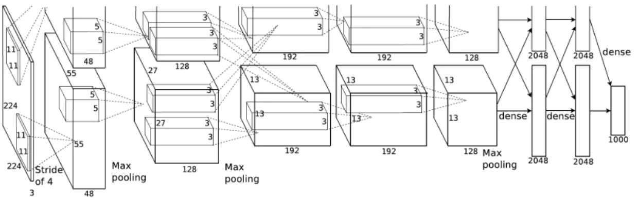
Figure 2.10: AlexNet Architecture

2.2.1.2 Architectures

There are many architectures presently used for image classification. For purposes of this

document, we will discuss the most profound accomplishments to the field of image classification.

Following the example of LeNet, one of the pioneer architectures of the field of computer vision

(image classification, in general) is AlexNet [25] created by Alex Krizhevsky while working under

Geoffrey Hinton. AlexNet is composed of 5 convolutional layers that perform feature extraction and

then are followed by 3 fully-connected layers whose purpose is to output a classification percentage

for each of the 1000 classes in the form of a 1000-way softmax function. The output with the highest

classification percentage is taken as the object which is present in the image. Figure 2.10 illustrates

the architecture developed by Krizhevsky et al.; notice that the architecture is split into two separate

portions. The architecture is split due to computational limitations of the GPUs at the time of this

networks creation. Each half of the model was placed on difference GPUs and trained separately

(oddly enough, both sections learned their own independent features). The 11x11 blocks shown on

the far left of the image illustrate the convolutional filters that are learned throughout the training

process with an input image, in this case, of size 224x224x3 (i.e., an RGB image). The first layer

depicted (the bottom half of the first layer, to be more exact) is of size 48x55x5. This means that

there are 48 independent filters in this layer created by sliding the 11x11 convolutional kernel with a

stride of 4 (skipping 4 pixels every slide). Further the max pooling after this layer creates a smaller

dimensionality layer as well as attempts to filter out features that are not needed (i.e., feature that

aren’t edges, corners, etc.)

(33)

Figure 2.11: VGG Architecture

Figure 2.12: GoogleNet Architecture

for classification called VGG [26]. The key features that made this architecture revolutionary

are keeping the convolutional filters as simple as possible as well as growing the number of layers

significantly to 19 layers. Another main idea of this paper is to stack convolutional layers before

pooling rather than pooling after each layer (as AlexNet has done), while still being able to improve

the error rate to 7.3% on the ImageNet challenge. Figure 2.11 illustrates the VGG architecture

(notice the much smaller filters sizes creating nuch smaller convolutional layers).

Also in 2014, Szegedy et al. [27] went with a different strategy which was creating a more

complex architecture, naming it GoogleNet(depicted in Figure 2.12). One of the main

contribu-tions of this architecture is it’sInception module which is able to process inputs in parallel through multiple 1x1 and 3x3 convolutions. Although the architecture is much bigger and more complex

than previous architectures, it minimizes the total number of parameters, therefore speeding up

inference time.

Lastly, one of the most important innovations in recent years in image classification is the

(34)

Figure 2.13: ResNet Unit

deeper is the problem ofvanishing gradients. In short, the problem is that using the chain rule for back-propagation only works through a finite number of layers before the errors being propagated

are non-negligible. To combat this problem, Kaiming He et al. showed that by inserting a

skip-connection in the architecture, the optimization is able to learn a residual mapping instead of the

mapping itself. This architecture won the ImageNet 2015 Challenge with 152 layers and a residual

unit is shown in Figure 2.13.

2.2.2 Object Detection

While image classification has been well studied over the years and architectures have been

developed to perform extraordinarily well with this task, there are many instances where simply

identifying the objects in an image is not enough. The bulk of this dissertation is based on this

concept. Rather than simply stating that a particular image contains a "dog", we would like a

system that both says there is a "dog" and the dog is located at (x1, y1),(x2, y2)position in the

image. However, we can not simply use the same architectures that were used for image

classifi-cation because the output for these networks are softmax probabilities which include no loclassifi-cation

information. Although it is not done this way in practice, we can think of object detection as an

extension of image classification where we develop a heat map where objects could potentially be

located in the image and then classify each of the areas as either an object or not. Another way

to think of the object detection problem is to have a sliding window go over the entire image and

pass each window through a classifier. In this section we will discuss in detail a few architectures

which have come to be the state-of-the-art architectures for object detection as well as mention a

(35)

2.2.2.1 Datasets

COCOis an object detection dataset developed by Microsoft standing for Common Objects in

Con-text. This dataset contains complex everyday scenes containing 91 objects in natural environments

with about 2.5 million images. There are many APIs that provide pre-trained models that have

been trained using the COCO dataset. These models are useful for using pre-learned features as

starting points for custom datasets.

Pascal VOCis another object detection dataset developed for "large scale" image classification and

detection. There are 500K images in this dataset consisting of about 20 classes of normal objects

(including vehicles, buildings, etc.) Again, there are many APIs that provide pre-trained model

trained on this dataset as a starting point for training with custom data.

KITTIis an autonomous driving detection dataset developed in a collaboration between University

of Toronto and KIT. This dataset contains objects that would be relevant for autonomous driving

models such as different types of vehicles, pedestrians, roads, etc. Not only does this dataset contain

object detection labels, but there are many other types of data including road segmentation, stereo

vision and lidar data for depth mapping, and optical flow dataset to track motion of objects. For

our purposes, we will only be using the detection aspects of this dataset.

There are many other datasets for object detection depending on the task at hand including

LISA (a traffic sign database), WIDER (a facial detection database), and ALPR (for license plate

recognition).

2.2.2.2 Architectures

Architectures that are currently being used for object detection are much different than

those being used for image classification (aside from the inherent backbone of convolutional layers).

Again, the main difference is that we are required to predict not only the class of the object but also

its location in the image which inherently involves more than a softmax probability layer.

The first recent technique that has been used for object detection does not involve a

convo-lutional network at all. In 2005, Dalal and Triggs [29] introduced the concepts of Histogram Oriented

Gradients (HOG) features which used a sliding window approach on a pyramid of scaled images.

For each scaled image, HOG features were calculated and then fed into a support vector machine

(36)

The development of HOG methods led directly to the creation of the first deep learning

based object detection, Region-based Convolutional Neural Networks (R-CNN) [30]. First, the same

strategy was employed as HOG, however, the SVM classifiers were replaced with CNNs. It was

impossible, however, at this time to run CNNs on so many image patches due to computational

limits. To circumvent this, R-CNN uses a technique called Selective Search which reduces the

number of bounding boxes that are given to the classifier significantly. Once the patches are fed to

the convolutional networks for feature extraction, they are then fed to SVMs to perform classification

as well as a bounding box regressor.

Next, Girshick developed a technique called Fast R-CNN [1] to alleviated one of the main

problems facing both R-CNN as well as other similar techniques: it was able to be trained in an

end-to-end fashion. One other addition that was made was combining the bounding box regression

into the neural network itself. This was accomplished by having two heads on the network: one

classification head and one bounding box regression head.

Still further improvements could be made by Girshick et al. when developing the newest

of the 2-phase networks, Faster R-CNN [2]. By far the slowest portion of the Fast R-CNN pipeline

was the Selective Search algorithm. To speed up the training process (as well as the inference

process), Faster R-CNN replaces the selective search component with a smaller CNN called the

Region Proposal Network (RPN). Figure 2.14 illustrates the Faster R-CNN architecture which is

still currently one of the highest performing architectures in terms of accuracy on datasets like Pascal

VOC while being 10 times faster than Fast R-CNN.

For all the aforementioned architectures (R-CNN, Fast R-CNN, and Faster R-CNN), the

object detection problem is broken down into a two stage pipeline where object proposals are

gener-ated throughout the image and then a classifier and regressor are run on each proposal to determine

its efficacy in the final output. However, on specific architectures (namely, embedded architectures),

this heavy pipeline is not suitable for running CNNs in real-time. For this reason, there have been a

few architectures developed that have been coined "single shot detectors" which look at the

detec-tion problem as a regression problem as a whole instead of a classificadetec-tion and regression problem

separately.

The first architecture which attempted a "single-shot" mentality was YOLO [4]. Standing

for "You Only Look Once" this detector was able to learn the class probabilities as well as bounding

(37)

Figure 2.14: Faster RCNN Architecture

that the former uses a set of object proposals to perform classification on while the latter uses a set

of grid boxes overlaid on the image with different aspect ratios to localize objects. In short, YOLO

divides the input image into a grid where each grid predicts N bounding boxes and corresponding

confidence values. Techniques such as non-maximal suppression and thresholding are then used to

remove extraneous boxes leaving behind the boxes which are best fit for the objects in the image.

Figure 2.15 illustrates the full YOLO pipeline. One advantage of YOLO over R-CNN methods is

seeing the entire image allows for contextual information to hinder the amount of false positives.

However, due to the limitation of of the architecture, sometimes it struggles to localize smaller

objects. More recently, [5] was published extending the YOLO model to not only execute faster but

also generalize much better; the new architecture design was able to detect up to 9000 classes of

objects.

Following YOLO, the second single-shot architecture was developed, namely Single Shot

Detection (SSD) [3]. SSD utilizes numerous great features from the YOLO architecture including

predicting boxes based on a grid cell system. Two of the major differences between YOLO and

SSD are that SSD predict off-sets based on grid cells rather than learning the box itself as well as

predicting boxes at multiple scales by taking outputs from many subsequent convolutional layers.

(38)

Figure 2.15: YOLO Example

Figure 2.16: SSD Architecture

from many different convolutional layers. The initial layers (VGG-16 layers) are used for feature

extraction while the following 5 convolutional layers are used for localizing objects of different aspect

ratios (layers closer to the input looking for smaller objects).

One of the major problems in developing and deploying deep learning architectures for object

detection in general is choosing the correct architecture to begin developing with. There is always

a trade-off when it comes to deep learning models between accuracy and speed. If an application

requires the fastest inference possible (for example, autonomous driving), an architecture that needs

to make object proposals for every image and then classify each one of those may not be fast enough.

On the other hand, for applications such as medical imaging where speed is not so important but

the more accurate prediction can lead to a better medical outcome may lend itself to a deeper

architecture.

2.2.3 Re-Identification

In contrast with image classification and object detection, the task of re-identification has

(39)

designing a system. Image classification involves simply stating the presence of an object or

item-of-interest in a given image. Object detection takes this one step further and not only identifies

the object but also localizes it within the image. The task of re-identification involves extracting

metadata (or a feature) from an already localized object for use with further processing (i.e. tracking,

surveillance, security, etc.). However, this is already what a traditional image classification network

is performing; feature extraction so that each class can be separated into its own portion of the

embedding space. The major difference in the task of classification and re-identification can be

illustrated by a problem involving hundreds of objects versus a problem containing millions of objects.

If there are only hundreds of classes (i.e. a dataset such as ImageNet), current networks have the

ability to use traditional softmax layers to create a model with the ability to decipher between

the classes easily. However, in the case of the million-class dataset (number of cars entering an

airport in a period of time), it is nearly impossible to find a current model capable of using softmax

classification to perform well. For this reason there are techniques that can be used to force objects

of different classes (even if they are almost the same object) to be separate in embedding space

representation. As most re-identification tasks utilize image classification networks, in this section

we will focus on the changes made to a network as well as the special training methods used for

creating a model capable of the aforementioned abilities as well as illustrate a few dataset that were

used in the later section to solidify our findings. The specific task of vehicle re-identification will be

studied in this work as the person re-identification is a much easier problem and is a well-studied

problem. The problem we will discuss is creating a feature (signature) for each of the vehicles in a

given dataset.

In video analysis, most higher level algorithms like action recognition and anomaly detection

rely on traditional methods likeMultiple Camera Multiple Object Tracking (MC-MOT); this method employs object verification (or re-identification) for gaining a confidence value to associate objects

across multiple videos [31]. All of the techniques utilized for re-identification can also be utilized in

single camera scenarios where the objective is determine if the same object appeared in the scene

more than once [32, 33, 34].

As we will be discussing vehicle re-identification as our application of choice, we will first

give a brief description followed by some of the unique characteristics that this application entails.

The task of vehicle re-identification is to identify the same vehicle as it travels across a camera

(40)

Figure 2.17: Samples from VeRi [9] Dataset (Each Row is Seperate Identity)

management systems have become more prevalent [35]. Previous works [36, 37] have shown the

ability to create a unique identifier based on license place information; however, in many scenes

that involve vehicles, the cameras are not placed in a manner in which the license plate is in view

from all angles. Therefore, vision-based re-identification is necessary to create a unique identifier

based on other aspects of the vehicle like appearance including viewpoint shifts/rotations, lighting

variations, and different poses. Figure 2.17 illustrates some of these aforementioned challenges in a

given dataset.

As mentioned before, vehicle re-identification brings about a few unique challenges when

compared to a traditional person re-identification application. A few of these challenges are as

follows:

1. In a system for vehicle re-identification, the labels are much more fine-grained than person or

face labels. Given that there are a finite number of colors and types of vehicles, the diversity

in the datasets is much less than other re-identification problems. This causes problems when

defining the difference between objects or vehicles.

2. Multiple views of the same vehicle must be semantically correlated and, therefore, the identity

of the given vehicle should be correctly decided aside from the viewpoint. Any approach to

(41)

all of this information separately to make decision about identity.

3. In any real-world environment, a re-identification system should be able to extract subtle

physical cues (or differences) in objects (in particular, things like dust, dents, etc. when it

comes to vehicles) to help distinguish between vehicles which have the same characteristics

otherwise (color, type, etc.). However, due to location of these anomalies, it could be difficult

to see them given the viewpoint from the camera. For this reason, in practice, there is also a

spatio-temporal matching piece that is employed to introduce a new parameter to distinguish

objects that are similar [40, 39].

In short, we first need to obtain an embedding for each of the objects. The embedding is then used

to perform a distance metrics which expresses the closeness of the objects in embedding space. Any

good embedding should be invariant to illumination, scale, and viewpoint changes, just to name

a few. Prior to advances in deep learning, most embeddings were handcrafted using a mixture of

multiple types of feature extractors or learning a ranking system for the objects of similar identities

[41, 42, 43, 44, 45, 46, 47].

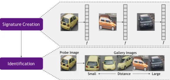
Figure 2.18 illustrates the overall pipeline for a vehicle re-identification problem. First we

have asignature extractor orcreator which creates the embedding discussed above. This embedding is then compared to the other objects which the system knows about (a.k.a. that gallery). The gallery is made up of all other images in the systems world. Theprobe image is then compared to each one to decide which other vehicle it is closest (hopefully the same vehicle identity). The order

of the gallery images in Figure 2.18 shows an optimal ranking of thegallery images after a correctly trained feature extractor has been created. Notice that the gallery images with the smallest distance

from theprobe image are the same vehicle and even close to the same pose while the larger distance ones are of other vehicles.

2.2.3.1 Datasets

VeRiis proposed in [9] is one of the first datasets created solely for the task of vehicle re-identification.

This dataset encompasses 40,000 bounding box annotations of 619 vehicle (identities) across 20

cam-eras in traffic surveillance scenes. Each vehicle is captured in 2-18 camcam-eras in various viewpoints

and varying illuminations. Notably, the viewpoints are not restricted to only front/rear but also side

(42)

Figure 2.18: Re-Identification Process for Creating Embeddings for Objects

(a) VeRi Dataset [9] (b) VehicleID Dataset [39] (c) PKU-VD Dataset [48]

Figure 2.19: Vehicle Re-Identification Datasets

make and model of vehicles, color, and inter-camera relations and trajectory information. A few

example images from the VeRi dataset can be seen in Figure 2.19a.

vID is proposed in [39] comprises 221,763 bounding box annotations with a much larger group

of identities (26,267) and are captured across various surveillance cameras in a city. Annotations

include 250 vehicle models as well as having an order of magnitude more identities than the VeRi

dataset. However, the viewpoints only include front and rear views for the vehicles. A few example

images from the VeRi dataset can be seen in Figure 2.19b.

PKU-VDis proposed in [48] and is the newest and largest of the vehicle re-identification datasets.

This dataset comprises about two million images and their fine grained labels including vehicle

model and color. This dataset is split into two sub-datasets, namely VD1 and VD2 based on cities

from which they are captured. The images in VD1 are captured from high resolution cameras while

(43)

in VD1 and VD2, respectively. A few example images from the VeRi dataset can be seen in Figure

2.19c.

2.2.3.2 Architecture and Loss Function

As mentioned previously, most retrieval or re-identification networks are based on traditional

image classification network designs. For example, many of these networks have a backbone of a

typical network like VGG [26], ResNet [28], MobileNet [49], or one of the other normal image

classification networks. The main difference between typical classification networks and a network

used for re-identification is the last few layers of the network. Firstly, one of the main challenges

with re-identification problems is the large number of classes that need to be identified. In most

image recognition tasks there are hundreds or even thousands of objects (in the case of ImageNet)

which would need to be identified. However, in the task of re-identification, the objects can easily

scale to tens of thousands or even millions of identities. For this reason, a traditional softmax

classification layer will not be able to handle this type of data. Furthermore, in the task of retrieval

or re-identification we are not necessarily trying to find an exact class, but rather compare the

feature that we have extracted to another known object.

In a typical architecture for re-identification, the object is presented to a feature

extrac-tor followed by an identification portion which consists of a fully connected layer and an optional

normalization layer. Instead of them passing this result to a fully-connected layer to identify the

object, thesignature is taken from this portion of the network to perform distance comparisons in embedding space. But the question is, without a softmax classification layer, how is the network

trained to be able to recognize differences in the objects of different identities? The answer that

we have come up with for this question is to utilize manifold learning with triplet loss as well as

different sampling techniques to optimize the loss value while training.

Consider a datasetX ={(xi, yi)}Ni=1ofNtraining imagesxi∈RDand their corresponding

class (identity) labelsyi∈ {1· · ·C}. Re-identification approaches aim to learn an embeddingf(x;θ) : RD_→

RF _{to map images in}

RD_{onto a feature (embedding) space in}

RF_{such that objects of similar}

identity are metrically close in this feature space.

Let D(xi, xj) : RF ×RF → R be a metric measuring distance of images xi and xj in

embedding space. For simplicity we drop the input labels and denoteD(xi, xj)as Dij. A value of