Approximation algorithms for clustering and facility location problems

(1)

c

(2)

APPROXIMATION ALGORITHMS FOR CLUSTERING AND FACILITY LOCATION PROBLEMS

BY

SHALMOLI GUPTA

DISSERTATION

Submitted in partial fulfillment of the requirements

for the degree of Doctor of Philosophy in Computer Science

in the Graduate College of the

University of Illinois at Urbana-Champaign, 2018

Urbana, Illinois

Doctoral Committee:

Professor Chandra Chekuri, Chair

Assistant Professor Karthekeyan Chandrasekaran

Professor Sariel Har-Peled

Professor Sheldon H. Jacobson

(3)

Abstract

In this thesis we design and analyze algorithms for various facility location and clustering problems. The problems we study are NP-HARDand therefore, assuming P6=NP, there do not existpolynomial time algorithms to solve them optimally. One approach to cope with the intractability of these problems is to designapproximation algorithmswhich run in polynomial-time and output anear-optimalsolution forallinstances of the problem. However these algorithms do not always work well in practice. Often heuristics with no explicit approximation guarantee perform quite well. To bridge this gap between theory and practice, and to design algorithms that are tuned for instances arising in practice, there is an increasing emphasis onbeyond worst-case analysis. In this thesis we consider both these approaches.

In the first part we design worst case approximation algorithms for UNIFORMSUBMODULARFACILITY

LOCATION(USFL), and CAPACITATEDk-CENTER(CAPKCENTER) problems. USFL is a generalization of the well-known UNCAPACITATEDFACILITYLOCATIONproblem. In USFL the cost of opening a facility is a

submodular function of the clients assigned to it (the function is identical for all facilities). We show that a natural greedy algorithm (which gives constant factor approximation for UNCAPACITATEDFACILITY

LOCATIONand other facility location problems) has a lower bound ofΩ(logn), wherenis the number of clients. We present anO(log2k)approximation algorithm wherekis the number of facilities. The algorithm is based on rounding a convex relaxation. We further consider several special cases of the problem and give improved approximation bounds for them. The CAPKCENTERproblem is an extension

of the well-knownk-center problem: each facility has a maximum capacity on the number of clients that can be assigned to it. We obtain a 9-approximation for this problem via a linear programming (LP) rounding procedure. Our result, combined with previously known lower bounds, almost settles the integrality gap for a natural LP relaxation.

In the second part we consider several well-known clustering problems like k-center, k-median, k-means and their corresponding outlier variants. We use beyond worst-case analysis due to the practical relevance of these problems. In particular we show that when the input instances are 2-perturbation resilient (i.e. the optimal solution does not change when the distances change by a multiplicative factor of 2), the LP integrality gap fork-center (and also asymmetric k-center) is 1. We further introduce a model of perturbation resilience for clustering with outliers. Under this new model, we show that previous results (including our LP integrality result) known for clustering under perturbation resilience also extend for clustering with outliers. This leads to a dynamic programming based heuristic fork-means with outliers (k-MEANS-OUTLIER) which gives an optimal solution when the instance is 2-perturbation resilient. We propose two more algorithms fork-MEANS-OUTLIER— a sampling based algorithm which

gives anO(1)approximation when the optimal clusters are not “too small”, and an LP rounding algorithm which gives anO(1)approximation at the expense of violating the number of clusters and outliers by a small constant. We empirically study our proposed algorithms on several clustering datasets.

(4)

(5)

Acknowledgments

This thesis would not have been possible without the help and support of a number of people. First and foremost, I would like to thank my advisor, Prof. Chandra Chekuri, for his persistent guidance and infinite patience. He was encouraging and supportive throughout the years, especially at times when I was frustrated with the lack of research progress and was uncertain of myself. His door was always open for me, and his insights and invaluable feedback have contributed immensely towards my research, writing, and presentation skills. I am truly grateful to have had a mentor like Chandra — his passion for learning and teaching, approach to research, innate humility and sense of fairness will always be an inspiration.

I would like to thank my other committee members, Prof. Karthik Chandrasekaran, Prof. Sariel Har-Peled, Prof. Sheldon Jacobson, and Dr. Maxim Sviridenko for their time, support and helpful comments. I am very grateful to all my co-authors, collaborators, and internship mentors; I have learned a lot working with them. Many thanks to Dr. Eyal Amir for his mentorship, I could always count on him for sound advice on research, career, and life in general. I would also take this opportunity to gratefully acknowledge the financial support from Prof. Chandra Chekuri’s NSF grants CCF-1319376 and CCF-1526799.

I would like to thank all the faculty and students of the UIUC theory group. In particular, I am grateful to Prof. Sariel Har-Peled for his teaching, advice, and support. It was always enjoyable talking to Sariel, and I will fondly remember his “hello-hello-shalom-shalom”s for years to come. Special thanks to my wonderful colleagues and office mates over the years: Matthew Bauer, Hsien-Chih Chang, Konstantinos Koiliaris, Nirman Kumar, Patrick Lin, Vivek Madan, Kent Quanrud, Benjamin Raichel, Yipu Wang, Chao Xu — the stimulating and often bizarre conversations were always a welcome break! I would also like to thank the administrative staff in the Department of Computer Science for helping me navigate the plethora of official rules and deadlines.

Life in UIUC would have been much less interesting and enjoyable without my friends. Debapriya, Sreeradha, Swarnali, Srijan, Sourabh, Ankita, Utsav, and Piyush — the coffee and chai, the good food, the Durga Puja, the trips, watching FRIENDS for the hundredth time, solving world problems over late-nightaddas— I will forever cherish the countless joyful moments I spent with you. Thanks for making this place a home away from home.

I am truly blessed to have the most wonderful family. Their unconditional love and support over the years have played an indispensable role towards my growth as a person, and in my career. Hope I can always make you proud.

Finally, my love and thanks go to Mainak, for being an amazing partner and friend. Thank you for putting up with me and being there for me in the best and worst times. Your constant encouragement, optimism, calm demeanor, and cool-headed advising helped me through some of the most tumultuous moments. Most of all, thank you for all the laughter. This incredible journey would have been incomplete with you.

(6)

Introduction

Many real-world problems, such as warehouse placement, routing vehicles, scheduling jobs, can be modeled as discrete optimization problems. Unfortunately, many of these problems are NP-HARD.

Thus, unless P=NP, there do not existefficient(polynomial time) algorithms to solve them optimally. A common approach to designing efficient algorithms for NP-HARDproblems is to relax the requirement of

finding an optimal solution. Such algorithms, known asapproximation algorithms, run in polynomial time, but instead of producing the optimal solution, they return a feasible solution which is guaranteed to benear-optimal, i.e., a solution whose value is within a small multiplicative factor (calledapproximation ratio) of the optimum value. Approximation algorithms have been extensively studied for a wide variety of NP-HARD problems[101,105].

For several NP-HARDproblems, in practice, heuristics often return exceptionally good solutions, which are much closer to the optimal solution than indicated by the best approximation guarantees known for these problems. One reason is thatworst-caseorhard instancesare often contrived and may not arise in real applications. Thus worst-case analysis is often overly pessimistic of an algorithm’s performance on typicalinstances or real world instances. The motivation to better understand real instances, and design algorithms by exploiting the structural properties of these instances has inspired the so-calledbeyond worst-case analysis of algorithms(BWCA). In a rapidly developing line of work by the algorithms community, various models have been proposed to abstract real instances, such as, input being generated from some distribution or optimal solution being significantly better than other candidate solutions. Algorithms have been proposed for these models and have led to numerous positive results[96].

In this thesis we consider discrete optimization problems through the lenses of both worst-case and beyond worst-case analysis. The problems we consider can be broadly categorized as the facility location (FL) problems. FL problems form an important class of combinatorial optimization problems and have been widely studied in computer science and operations research since the early 1960’s. These problems can be characterized by four common elements:

• A set of locations wherefacilitiesmay be opened. There can be a cost associated with opening a facility – calledfacility cost.

• A set ofclientswhich need to be served. There is a cost associated with serving a client, typically measured by the distance between the client and the facility to which it is assigned – frequently calledassignmentorconnection cost.

• A list of constraints which are imposed on the open facilities or client assignment. For e.g., a fixed number of facilities may be opened, or clients may need to be assigned to multiple facilities.

(8)

• A cost function measuring the quality of solution, which depends on the open facilities and client assignment.

The goal in FL is to determine a set of facilities to open and an assignment of clients to these open facilities such that all the constraints are satisfied while minimizing the cost function. Some well-known problems in FL are UNCAPACITATEDFACILITYLOCATION,k-median, andk-center.

In UNCAPACITATEDFACILITYLOCATION(UncapFL) problem, we are given a set of facilities, a set of clients, and metric distance functiond defined over the facilities and clients. Additionally, each facilityi has a fixed opening cost of f_i. The goal is to open a subset of facilities so as to minimize the sum oftotal facility cost(sum of facility cost of open facilities) and thetotal connection cost(sum of distances from each client to its nearest open facility).

In contrast to UncapFL, ink-center andk-median, there is no facility opening cost, instead there is a restriction that at mostkfacilities can be opened. The objective is to minimize the (1) maximum distance between a client and the nearest open facility (k-center); (2) sum of distances of clients to nearest open facility (k-median).

There is a rich body of literature on UncapFL,k-median, andk-center problems, and constant factor approximation algorithms are known for all three — resp. 1.488[77], 2.675[32], 2[57,66]. A wide variety of techniques have been employed to design and analyze the algorithms: (1) filtering[80,98]; (2) primal-dual[70]; (3) local search [15,59,73]; (4) greedy[57,65,66,68,69]; (5) LP rounding

[35,46,78,99]. On the negative side, it is hard to approximate UncapFL,k-median,k-center within a factor of 1.463[58], 1+2/e[69], 2 resp. We refer the interested reader to the following survey papers for more detailed overview[1,88,103].

While the UncapFL problem finds its application mainly in industrial situations (like warehouse placement), thek-median andk-center problems are studied more in the context ofclustering. The goal of clustering is to partition the input objects into groups such that objects in the same group are similar. To this end, often objects are represented as points in a metric space, and similarity is measured in terms of distance between them. Since clustering is one of the main motivations behind studyingk-median andk-center, in literature for these problems, the input is not separated into clients and facilities. The input is simply a set of points or vertices in metric space, andkof them are chosen ascentersto minimize the assignment cost. Further, clustering has motivated studying these problems in fixed dimensional Euclidean space as well (refer to[2,30,44,54], and references therein).

k-means — a closely related problem, is widely used by the Machine Learning and Data Mining community for various clustering applications. Here the goal is to choosekpoints as centers, such that sum ofsquared distanceto the nearest center is minimized. Although various approximation algorithms are known for this problem[6,71](including the ones fork-median which extend to this problem), they are rarely used in practice. Most of these algorithms conceptually too involved to find wide-spread use. The most commonly used algorithm is in fact a simple heuristic called Lloyd’s algorithm[81], which although has no explicit guarantee, performs remarkably well on real data with careful initialization[14].

(9)

Thus for clustering there is a gap between what isknownin theory and what is actuallyusedin practice. In fact thek-means problem, and clustering in general, is one of the driving forces behind BWCA.

The central theme of this thesis is design and analysis of algorithms for various FL problems. However, philosophically there are two parts to it. In the first part (Chapter2, Chapter3) we consider some natural generalizations of FL problems (namely, UNIFORMSUBMODULARFACILITYLOCATIONand CAPACITATED k-CENTER) and design traditional approximation algorithms for them. The results are interesting primarily from a theoretical perspective. In the second part (Chapter4, Chapter 5) we take a more practical standpoint — we consider FL problems in the context of clustering (namelyk-median,k-means,k-center and their outlier variants), and design algorithms which have strong theoretical guarantees when the input satisfies some structural properties. However, the algorithms are simple enough to be used as heuristic in practice.

1.1 Preliminaries

In this section, we review some basic terminologies and definitions we use in different chapters. Definition1.1 (Non-negative function). Let f : 2V 7→Rbe a real-valued set function defined over a finite

setV. The function f isnon-negativeif f(A)≥0 for allA⊆V. Definition1.2 (Normalized function). Let f : 2V _7→

Rbe a real-valued set function defined over a finite

setV. The function f isnormalizedif f(;) =0.

Definition1.3 (Monotone function). Let f : 2V_7→Rbe a real-valued set function defined over a finite

setV. The function f ismonotoneif f(A)≤ f(B)for any two setsA,B⊆V such thatA⊆B. Definition1.4 (Submodular function). Let f : 2V _7→

Rbe a real-valued set function defined over a finite

setV. The function f issubmodularif, for allA,B⊆V we have

f(A) +f(B)≥ f(A∪B) +f(A∩B) (1.1) Equivalently, a submodular function can be defined as a set function exhibitingdiminishing marginal returns— the function f is submodular if, for any two subsetsA,B⊆V such thatA⊆Band any element v∈V\B, we have

f(A_∪(v))₋ f(A)_≥ f(B_∪(v))₋f(B) (1.2) A classical example of submodular function iscoverage function. We say f is a coverage function when elements ofV are sets over some other ground setX, and f(A) =

S v∈A v .

Definition1.5 (Metric). A metric on a setV is a function d :V ×V 7→R_≥0 (also called the distance function), such that the following three properties are satisfied: (1)d(u,v) =0 if and only ifu=v; (2) (symmetry)d(u,v) =d(v,u)for allu,v∈V ; (3) (triangle-inequality)d(u,v) +d(v,w)≤d(u,w)for all u,v,w∈V .

(10)

Definition1.6 (Metric space). A metric space is defined as anordered pair(V,d)whereV is a non-empty set andd is a metric defined overV.

Definition1.7 (Integrality gap). For a minimization problemπ, the integrality gap for a linear program-ming L P is sup

I∈π

OPT(I)

OPT_{L P}(I), where OPT(I)and OPTL P(I)are respectively the integral optimal value and fractional optimal value forI. That is, the integrality gap is the worst case ratio over all instancesIofπ, of the integral optimal value and the fractional optimal value.

For a maximization problem, integrality gap is defined as the supremum of the inverse ratio.

1.2 Thesis Outline

Below we provide a high level overview of problems we consider in this thesis and our contribution.

1.2.1 Uniform Submodular Facility Location

Consider the scenario where a grocery store chain wants to determine the most effective locations in a city to open outlets. The company has done a market survey to get an idea of the monthly grocery list of each household. The operational cost of an outlet depends on the different types of products it carries. The problem of deciding where to open the outlets, and which products each individual outlet should carry such that the joint operational cost of the grocery store and average distance a customer has to travel for grocery shopping is minimized can be modeled as the UNIFORMSUBMODULARFACILITY

LOCATION(USFL) problem.

In USFL problem, we are given as input a set of kfacilitiesF, a set of nclientsD, a normalized monotone submodular facility cost function f : 2D→R₊, and a distance metricd defined onF∪D.

The objective is to partition the clients into sets_{S_i_}_i_∈_F, where client setS_i is assigned to facilityi, such that P i∈F f(Si) + P i∈F P j∈Si d(i,j)is minimized.

This is a special case of the SUBMODULARFACILITYLOCATION(SFL) problem, in which the submodular facility cost functions can be different for each facility. SFL has been previously considered by Svitkina and Tardös [100], Chekuri and Ene [40]. They gave an O(logn)-approximation for the problem. Further,[100]also showed that this approximation is best possible via an approximation preserving reduction from the SETCOVERproblem. A natural question is whether USFL is any easier to approximate.

We show that a natural greedy algorithm has a lower bound of Ω(logn)for USFL. The same greedy algorithm is known to yield anO(1)approximation for various facility location problems[62,68]. Thus our negative result demonstrates the difficulty of the problem. On the positive side, we give anO(log2k) approximation for USFL via a natural convex relaxation. At first glance this result seems weaker than the O(logn)approximation known for the more general SFL problem. However, known hardness results for the SETCOVERproblem, preclude any polylog(k)-approximation for SFL. Thus our result distinguishes

(11)

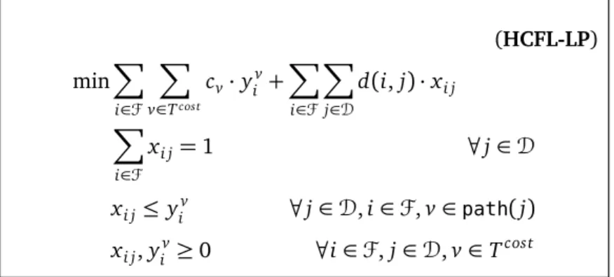
We also consider a special case of USFL known as HIERARCHICALCOSTFACILITYLOCATION(HCFL). Here, the facility cost function is given by a rooted tree Tcost, whose set of leaves is D. Each node v∈Tcost has a non-negative costc_v. Letpath(v)denote the unique path from nodev to the root of the tree. The facility cost function for a subsetS _⊆Dis f(S) = P

v∈S

j∈S

path(j)

c_v. Svitkina and Tardös[100] gave anO(1)approximation for this problem via an intricate local search based algorithm. We present a simpler LP rounding based algorithm, which has an approximation bound ofO(logk). Our algorithm is conceptually much simpler, and the benefit of an an LP rounding based approach is that it easily extends to a more general case where the facility cost function for a facilityiis given by f_i(S) = f(S) +h_i (here h_i is a fixed cost and can differ for facilities).

The details are in Chapter2, which is based on a manuscript with Chandra Chekuri.

1.2.2 Capacitated

k

-center

Suppose Amazon wants to setup fixed number of pickup locations in a city. It has shortlisted potential locations, and each location has a maximum capacity constraint on the number of customers it can manage (which can depend on factors like the number of lockboxes it can install at that location, number of employess etc). Further, Amazon knows the number of active Prime Members in each neighborhood. The problem of deciding, where to setup the pickup locations and how to assign each neighborhood to a pickup location without over-congesting them, and at the same time ensuring customer satisfaction i.e. each Prime Member has a pickup location in vicinity can be modeled as the CAPACITATEDk-CENTER

(CAPKCENTER) problem.

Formally in CAPKCENTER, the input consists of a set of verticesV, a distance metricd, a non-uniform capacity function L:V _7→Z+ defined onV, and a parameterk. The objective is to choosekvertices as centers, along with an assignment of every vertex to an open center which minimizes the maximum distance between a vertex and the center it is assigned to while honoring the capacity constraints: i.e., no open centervis assigned more vertices than its capacity L(v).

Although k-center admits an easy 2-approximation[66], the capacitated version of problem i.e. (CAPKCENTER) is much harder to approximate. In fact the natural LP relaxation has an unbounded integrality gap. Cygan, Hajiaghayi, and Khuller[50], obtained the first constant factor approximation for the CAPKCENTERproblem. Their algorithm works by preprocessing the instance to overcome the unbounded integrality gap of the natural LP relaxation, followed by an involved rounding procedure. The approximation factor is not computed explicitly, but is estimated to be roughly in the hundreds. We present a much simpler and clean rounding procedure (following the preprocessing step of[50]) to obtain a 9-approximation. It is known the integrality gap of the LP (after preprocessing) is at least 7[50]. Thus, our result almost settles the integrality gap: it is either 7, 8 or 9.

(12)

1.2.3 Clustering under Perturbation Resilience

In clustering we are givennpoints in metric space, and the goal is to partition them intokclusters such that some objective function measuring the quality of clusters is minimized. Thek-center,k-median, and k-means are arguably the most popular and well-studied clustering objectives. Althought the problems are known to be NP-HARD, many heuristic algorithms like Lloyd’s algorithm work quite well in practice. Several models have been proposed to understand real-world instances and why they may be computationally easier. One such model is based on the notion ofinstance stabilityorperturbation resilience, introduced by[17,28]. An instanceIis said to beα-perturbation resilient for someα >1 if the optimum clustering remains the same even if pairwise distances between points are altered by a multiplicative factor of at mostα.

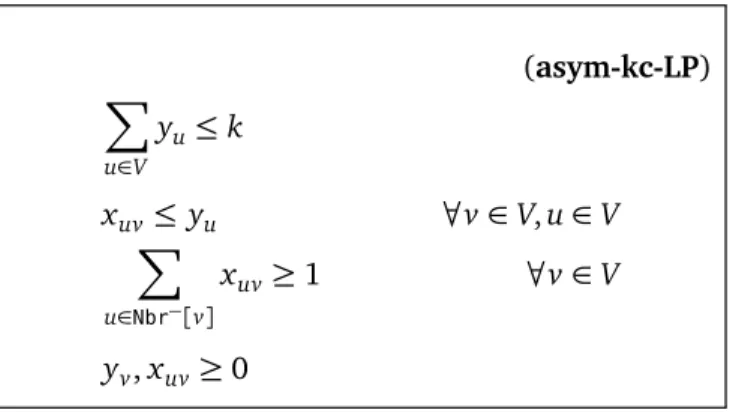
After several papers [17,23,24], a recent breakthrough result by Angelidakis, Makarychev and Makarychev[12]showed that 2-perturbation resilient instances of several clustering problems with center based objectives (which includesk-median,k-center,k-means) can be solved exactly in polynomial time. The algorithms proposed so far are combinatorial in nature. In this thesis, we attempt to understand the structure of the Linear Programming (LP) solution for these instances. In particular, fork-center (and asymmetrick-center) we prove that the LP is integral for 2-perturbation resilient instances. The result is interesting because it gives a new guarantee: when running the LP on ak-center (or asymmetric k-center) clustering instance, either we are guaranteed to have found the optimal solution (if the LP solution is integral), or we are guaranteed that the instance is not 2-perturbation resilient (if the LP solution is not integral). The previous algorithms known for this problem do not have this guarantee and can be arbitrarily bad if the instance is not perturbation resilient.

We introduce a model of perturbation resilience for clustering with outliers (see the next section for definition). We show that results previously known for clustering under perturbation resilience (including our LP integrality result) can be extended to clustering with outliers under this new model.

The details are in Chapter4, which is largely based on the paper[41].

1.2.4 k

-means with Outliers

The goal of clustering is to partition the input data intokgroups, such that data belonging to same cluster are similar. The problem is often abstracted as thek-means problem. The effectiveness ofk-means hinges on the assumption that the input data can be naturally partitioned intokdistinct clusters, which is often an unrealistic assumption in practice. Real-world data typically has background noise, and the k-means clustering is extremely sensitive to it. Noise can drastically change the quality of the clustering solution and it is important to take this into account in designing algorithms for thek-means objective. This motivates thek-means with outliers (k-MEANS-OUTLIER) problem. In this version of the problem,

the clustering objective isk-means, but the algorithm is additionally allowed to discard a subset of data points from the input. These discarded points are labeled asoutliersand are ignored in the objective, thus allowing the clustering algorithm to focus on correctly partitioning the bulk of the dataset that is

(13)

potentially noise-free and can be cleanly separated.

Formally, ink-MEANS-OUTLIER, we are given a set of points V, a metric distance functiond defined overV, and integer paramtersk,z. The goal is to find a set of kcentersC ⊆V, and a set of outliers Z_⊆V, with_|Z_{| ≤}z, such that P

p∈V min

c∈C d

2₍_p,_c₎_{is minimized.}

Although several bicriteria, and constant factor approximation algorithms are known for this problem

[36,43,56,61,74], they have not found use in practice. Unlikek-means, not many heuristics are known (except[38]which is a straight-forward extension of LLoyd’s). Designing practical algorithms has remained a challenging open question. We propose three algorithms — (1) a sampling based algorithm which gives constant factor approximation under mild size constraint on optimal clusters, (2) an LP rounding based algorithm which gives a constant factor at the expense of creating a few extra centers and outliers, (3) a dynamic programming based algorithm which can exactly solve the problem if the instance is perturbation resilient. We evaluate these algorithms on real data.

(14)

Chapter 2

Uniform Submodular Facility Location

2.1 Introduction

Svitkina and Tardös[100]introduced the SUBMODULARFACILITYLOCATION(SFL) problem: the input consists of a set ofkfacilitiesF, a set ofnclientsD, and for each facilityi∈F, a normalized monotone submodular facility cost function f_i: 2D→R+, and a distance metricd defined onF∪D. The objective is to partition the clients into sets_{S_i_}_i_∈_F, where client setS_i is assigned to facilityi, such that the sum of facility costandconnection costis minimized. Formally the goal is to minimize: P

i∈F fi(Si) + P i∈F P j∈Si d(i,j). The well-known UNCAPACITATED FACILITY LOCATION (UncapFL) problem is a special case of SFL; it is obtained by setting f_i(S) = h_i for all non-emptyS _⊆ D. Svitkina and Tardös gave an O(logn) -approximation for SFL via a greedy algorithm. Moreover, via a reduction from the SET COVERproblem,

they showed that SFL is Ω(logn)-hard. Subsequently, Chekuri and Ene [40] in the context of the SUBMODULARCOSTALLOCATION(SCA) problem, described a convex programming relaxation for SFL

based on the Lovász-extesion of submodular functions. They showed that this relaxation has an integrality gap ofO(logn)for SFL. It is worth noting that in the general setting ofS F L, the distance functiond on F∪Dneed not be a metric; any non-negative distance function can be captured by the non-uniform submodular functions and we can in fact simply consider the objective function P

i∈F

f_i(S_i).

In this chapter, we consider the case when the facility cost functions are identical i.e. f_i = f,∀i∈F, where f is a normalized monotone submodular function. We call this the UNIFORM SUBMODULAR

FACILITYLOCATION(USFL) problem. That is, the objective is to minimize: P i∈F

f(S_i) +P i∈F

P

j∈Sid(i,j)

under the assumption thatdis a metric. USFL is NP-HARDand APX-HARDeven for this special case since

it generalizes the UncapFL problem with uniform facility cost.

It is natural to ask the question if a uniform cost function across all facilities makes the problem easier to approximate. For some specific submodular functions constant factor is known; Svitkina and Tardös gave an O(1)-approximation for a special case called the HIERARCHICAL COST FACILITY

LOCATION (HCFL)[100]based on an involved local-search algorithm. Even for the CONCAVE COST

FACILITYLOCATION(CCFL) problem, where facility cost is a concave function of the number of clients assigned to it, a constant factor is known via a simple greedy algorithm whose analysis is based on dual-fitting[62](infact their result holds for the more general case, where each facility has a different concave cost function). One can consider a simple generalization of CCFL: each client j∈Dhas a weight w_j and now each f is a concave function of the total weight of clients assigned to it. Even in this case, we can get a constant approximation via a simple reduction to UncapFL.

(15)

on the following questions:

Question 2.1. Is there a constant factor approximation for USFL?

Question 2.2. Is the integrality gap of the Lovász-extension based relaxation for USFL O(1)?

To better understand the Lovász-extension based relaxation for USFL and provide some insight into the difficulties of rounding the relaxation, we consider the special case of HIERARCHICALCOSTFACILITY

LOCATION(HCFL) problem. Here, the facility cost function is given by a rooted treeTcost, whose set of leaves isD. Each node v ∈Tcost has a non-negative cost c_v. Letpath(v)denote the unique path from node vto the root of the tree, andparent(v)denote node v’s parent in Tcost. The facility cost function for a subsetS⊆Dis f(S) = P

v∈S

j∈S

path(j)

cv. In other words, the facility cost of assigning a subset of clients is given by the cost of the subgraph ofTcost induced by the nodes that lie on a path from the root to some leaf inS. As we mentioned earlier, Svitkina and Tardös presented a local-search based O(1) approximation algorithm for this problem[100](referSection 2.1.2 for more on HCFL). The Lovász-extension based relaxation and the natural LP relaxation are equivalent for HCFL. This raises the question:

Question 2.3. Is the integrality gap of the natural LP relaxation for HCFL O(1)?

The preceding questions are challenging. There has been no concrete evidence so far to suggest that ano(logn)approximation is possible for USFL. In this work we make some progress in answering these questions, and provide some insight into the difficulty of approximating USFL.

Remark. It is useful to consider a special case of SFL that is more general than USFL. This is obtained by allowing the fi to be different but in a limited way; each functionfi is of the form fi(S) =hi+f(S) whereh_i is a fixed cost for opening the facilityi, and f is a common submodular function. Questions2.1 and2.2are relevant for this more general class. Some of our results hold in this more general setting.

2.1.1 Results

One of the simplest algorithms for UncapFL is a simple greedy algorithm. Jain et al. [68]used an elegant dual-fitting analysis to prove that this greedy algorithm gives anO(1)-approximation for UncapFL and also establishes anO(1)integrality gap for the LP relaxation. The greedy algorithm also gives anO(1)-approximation for CCFL[62]. Note that this is the same greedy algorithm that gives an O(logn)-approximation for the much more general SFL problem that captures the Set Cover problem. It is natural to consider the greedy algorithm for USFL. We consider a special case of USFL: for any subset of clientsS_⊆D, f(S) =min P j∈S w_j,B

wherew_j’s are weight of each client j_∈D, andBis a constant. Surprisingly we show a lower bound ofΩ(logn)on the performance of the greedy algorithm for this problem even when the metric onF∪Dplays no role (all distances are 0).

(16)

Theorem 2.1. There is anΩ(logn)lower bound on the performance of Greedy Algorithm for USFL. Our main result for USFL is the following theorem.

Theorem 2.2. There is an O(logk)-approximation for USFL when the metric onF_∪Dis a tree metric. For general metrics there is an O(log2k)-approximation. Here k=|F|is the number of facilities and the approximations are with respect to the Lovász-extension based relaxation.

At first glance the preceding theorem seems weaker than theO(logn)approximation known for the more general SFL problem. However, known hardness results for the SET COVERproblem[89]rule out an approximation that is poly-logarithmic inm, the number sets. Via the reduction from SETCOVERto SFL, one can rule out any polylog(k)-approximation for SFL.

Claim 2.1. For SFL there is no2log1−δc(k)k_{-approximation for any constant c}_<₁_/₂_{unless SAT can be decided} in timeexpO(2log1−δc(n)n)whereδ_c(n) =1/(log logn)c.

Thus,Theorem 2.2separates the approximability of SFL and USFL for the first time. Our algorithm and analysis to proveTheorem 2.2rely very much on the uniformity of the facility function, and the fact thatd is a metric.

Finally, we consider the HCFL problem, which is a special case of USFL. We consider the natural LP relaxation of the HCFL problem and show that the integrality gap isO(logk)via a simple randomized LP rounding algorithm, wherek=|F|.

Our approximation results hold for the more general case, where the facility cost function is given by f_i(S) =h_i+f(S), hereh_i is a fixed cost that depends on facilityi, and f is a monotone non-negative submodular function.

2.1.2 Related Work

There is a very large literature on UncapFL and many related problems including clustering problems such ask-median. Various techniques in approximation have evolved from this work. We refer the reader to[1,88,103]for surveys, books on approximation[101,105], and[77]for the current best known result of 1.488-approximation. SFL and USFL are more closely related to the uncapacitated facility location problems. The capacitated versions where facilites have a limit on the number of clients they serve are more closely related to convex cost functions. Local search techniques have been the main technique for capacitated problems[4,26,46,73,92]until recent work based on LP relaxations[10]. A relevant paper here is a constant factor approximation for universal facility location[84,104]which captures capacitated facility location as a special case.

Lovász-extension based relaxations have been fruitful for problems involving minimizing submodular costs in several settings; we refer the reader to [39,40,42,45,51,67]. In particular the relaxation from[40]on SCA is the main inspiration for this work.

HCFL generalizes the facility location problem with service installation costs introduced by Shmoys, Swamy and Levi[97], and Ravi and Sinha[94]— the cost function in this case is given by a two level

(17)

tree. Ravi and Sinha[94]showed that even in this two-level case, if the node costs are different for each facility the problem is set cover hard. Shmoys et al.[97]considered the case where the node costs are different for each facility, however there is an ordering on the facilities, such that for each earlier facility the node costs are less than a facility which comes later in the ordering. They gave a 6-approximation for this problem using primal-dual approach. For the case, when the cost tree is identical for each facility they gave an improved approximation bound of 2.391 using randomized rounding.

Svitkina and Tardos[100]extended the problem to the multiple-levels case, under the restriction that the facility costs are same for each facility. They gave a 4.237 approximation for this problem using an involved local search method. Observe, one can obtain anO(d)approximation using rounding approach of[97], whered is the depth of the cost tree. Thus, the main novelty of Svitkina et al.’s result is getting an approximation bound independent of the depth of the tree. We mention that HCFL can be cast as a rather special case of USFL where the submodular function is a weighted set coverage function.

Chapter Outline. The rest of the chapter is organized as follows: in Section 2.2we describe the Lovász-extension based relaxation of USFL; inSection 2.3we give an example to show that Greedy fails for USFL; inSection 2.4we present a primal rounding algorithm for USFL and prove an integrality gap ofO(log2k); InSection 2.5we describe the natural LP relaxation of HCFL and prove that the integrality gap of this relaxation isO(logk); Finally we conclude the chapter with some open problems inSection 2.6.

2.2 Mathematical Programming Relaxations

We describe the convex relaxation based on the Lovász-extension from[40]as well as an equivalent relaxation based on the notion of “stars”.

2.2.1 Lovász-extension based relaxation

Lovász-extension of Submodular Function. LetXbe a finite ground set of cardinalityn. An arbitrary set function f : 2X _→R, can be extended to the continuous domain by defining a function from the

hypercube[0, 1]n toRthat agrees with f on the vertices of the hypercube. One such extension is given

by the Lovász-extension, denoted by ˆf: ˆf(x) = Ef(xθ)=R₀1f(xθ)dθ, where, for a given vector x ∈[0, 1]n_, _xθ _{∈ {}_{0, 1}_}n _{is defined as} _xθ

j =1 if xj ≥θ, and 0 otherwise. Lovász proved that ˆf(x)is convex iff f is submodular[82].

An alternative equivalent definition of Lovász-extension is as follows: Definition2.1. Given a vector x ∈[0, 1]n_{, and let} _X ₌_{_i

1,i2, ...,in}such that xi1 ≥ xi2. . .≥ xin. Let

(18)

Here,α_j ≥0, andP_jα_j=1. Further for any x_i_j =Pn_k₌_jα_j. Then, ˆ f(x) = n X j=0 αj·f(Aj) (2.1)

In other words,{α_j}j gives a distribution over a chain of sets, such that the marginal probability of each element isx_i

j, and ˆf(x)is the expected value of f over this distribution. It is easy to see from

Definition 2.1, given x, the value of ˆf can be computed in polynomial time, via a value oracle for f. We will state and prove some properties of the Lovász-extension of a monotone submodular function for completeness.

Observation 2.1. Consider two vectors x,x0_∈[0, 1]nsuch that x0_≤x i.e. for every i_∈X,x_i0_≤x_i. If f is a monotone submodular function, then fˆ(x0)≤ fˆ(x).

Proof: For anyθ∈[0, 1], letX_θ ={i∈X :x_i≥θ}, andX_θ0 ={i∈X :x0_i≥θ}. Since x0≤x, for every θ∈[0, 1], we haveX_θ0 ⊆X_θ. The monotonicity of the submodular function f implies, f(X_θ0)≤ f(X_θ), ∀θ∈[0, 1]. The claim then simply follows from the definition of Lovász extension:

ˆ f(x)₋ ˆf(x0) = Z 1 0 f(X_θ)dθ₋ Z 1 0 f(X_θ0)dθ = Z 1 0 f(X_θ)−f(X_θ0) dθ ≥0

This completes the proof.

Observation 2.2. Given a vector x∈[0, 1]n _and_β_∈₍_{0, 1}_{], let X}

β ={i∈X :xi≥β}. If f is a monotone non-negative submodular function then, f(X_β)_≤ _β1 _·fˆ(x).

Proof: For anyθ _∈(0, 1], letX_θ ={i∈X:xi≥θ}. Note ifθ≤β, then Xβ⊆Xθ. Thus

ˆ f(x) = Z 1 0 f(xθ)dθ = Z 1 0 f(X_θ)dθ ≥ Z β 0 f(X_θ)dθ ≥ Z β 0 f(X_β)dθ =β·f(X_β).

(19)

In the above, the first inequality is due to non-negativity of f and the second is due to monotonicity.

Lemma 2.1. Given a vector x _∈[0, 1]n, andβ_∈(0, 1], consider the scaled vector ˆx_∈[0, 1]n, such that ˆ

xi=min{_β1 ·xi, 1}. If f is a monotone submodular function, then fˆ(xˆ)≤ _β1 ·fˆ(x).

Proof: Consider any vector ˆx ∈[0, 1]n. Letβ·xˆbe the vector obtained by scaling eachx_i by a factor ofβ. UsingDefinition 2.1, it is straightforward to see ˆf(ˆx) = _β1 _· fˆ(β· ˆx). Now consider a vectors x ∈[0, 1]n_{, and vector ˆ}_x _{be as specified in the lemma statement. Observe,}_β_·_ˆ_x _≤_x_{. Therefore using} Observation 2.1we get, ˆ f(xˆ) = 1 β ·fˆ(β·ˆx) ≤ 1 β ·fˆ(x). This completes the proof.

Lemma 2.2. Let x(1),x(2), . . . ,x(k)_∈[0, 1]n andβ_∈(0, 1], such that for every i_∈X , k P `=1 x(_i`)=1. Then f(X)≤ k P `=1 ˆ f(x(`)).

Proof: UsingDefinition 2.1of Lovász-extension we can write, k X `=1 ˆ f(x(`)) = k X `=1 n X j=0 α(_j`)·f(A(_j`))

That is we have a collection of setsA=_{A(_j`): 1_≤`_≤k, 0_≤ j≤n}with weights{α(_j`)_}_`_,_j. Consider an elementi_∈X, letA(i) =_{A_∈A:i_∈A_}be the sets which containi. Observe, the sum of weights of the sets inA(i)is 1, sincePk

`=1x (`)

i =1, we call this the marginal weight of elementiover the collectionA. We claim that we can uncross the collection A (and modify weights accordingly) such that the weighted value does not increase, and the marginal weight of each element remains unchanged. Consider two setsB,C ∈Asuch that neitherB⊂C, notC⊂B. Because of submodularity of f, we can replace B,C with B_∪C, B_∩C without increasing the cost (f(B) + f(C)_≥ f(B_∪C) + f(B_∩C)). Repeated application of this uncrossing application gives our claim.

Thus we can find a chain of setsA0with weight vectorw0such that, k X `=1 ˆ f(x(`))≥ X Y∈A0 w0_Yf(Y).

Observe, since the marginal weight each element is 1 andA0is a chain, we must haveA0=_{X}. Thus Pk

(20)

Lemma 2.3. Let x(1),x(2), . . . ,x(k)∈[0, 1]n_and_β_∈₍_{0, 1}_{]. Let X}

β ={i∈X :P`k=1x (`)

i ≥β}. If f is a monotone non-negative submodular function then, f(X_β)≤_β1Pk

`=1fˆ(x(`)).

Proof: For each vectorx(`), consider the scaled vector ˆx(`), where ˆx_i(`)=min_{_β1 _·x_i(`), 1_}for eachi∈X. ByLemma 2.1, k X `=1 ˆ f(ˆx(`))≤ 1 β · k X `=1 ˆ f(x(`)).

Now consider the vectors ¯x(`)≤ ˆx(`)for every`∈[k], where ¯x_i(`)=0 if i∈/X_β, else ¯x_i(`)≤ ˆx_i(`), such thatPk_`₌₁¯x_i(`)=1. SincePk_`₌₁ˆx_i(`)≥1 for everyi∈X_β, the vectors ¯x(`)are valid. ByObservation 2.1 we get, k X `=1 ˆ f(x¯(`))≤ k X `=1 ˆ f(ˆx(`))

Restricting the functions f and ˆf on setX_β, and usingLemma 2.2we get,

f(X_β)≤ k X `=1 ˆ f(x¯(`)) ≤ k X `=1 ˆ f(xˆ(`)) ≤ 1 β · k X `=1 ˆ f(x(`))

This completes the proof.

Relaxation via Lovász-extension. We can define a relaxation for USFL via the Lovász extension. In what follows, we useito index the facilities inF, j to index the clients inD. For eachiand j, there is a variablexi j, which is 1 if client jis assigned to facilityi. Let vector x(i)denote then-dimensional vector obtained by considering the variablesx_{i j},j∈D. The relaxation is as follows:

(USFL-REL) minX i∈F ˆ f(x(i)) +X i∈F X j∈D d(i,j)·xi j X i∈F x_{i j}=1 ∀j∈D x_{i j}_≥0 _∀i_∈F,j_∈D

(21)

The preceding relaxation is a specialization of the relaxation in[40]for the SCA problem which is equivalent to SFL in the monotone case. In SCA the objective function is changed toP_i_∈_Fˆfi(x(i)).

2.2.2 The “star” relaxation

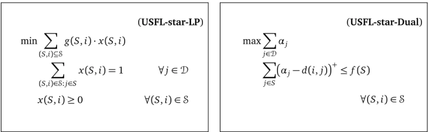
We now describe a different relaxation. A starconsists of a facility i and a setS of clients. Let S = 2D_×F denote the set of all possible stars. One can view the allocation problem as finding a collection of stars that cover all the clients. We can express this as an IP relaxation by considering the collection of 0, 1 variables x(S,i)for each star(S,i)_∈S. We assign a cost g(S,i)to(S,i), where g(S,i) =f(S) +P_j_∈_Sd(i,j). The allocation problem requires that each client jis assigned to exactly one star. (In the monotone submodular function setting one can relax this to require that each client jis required to be assigned to at least one star.) Based on this we obtain the following LP relaxation and the corresponding dual. (USFL-star-LP) min X (S,i)⊆S g(S,i)_·x(S,i) X (S,i)∈S:j∈S x(S,i) =1 _∀j∈D x(S,i)_≥0 ∀(S,i)_∈S (USFL-star-Dual) maxX j∈D αj X j∈S αj−d(i,j) + ≤ f(S) ∀(S,i)∈S

Figure 2.2: LP relaxation and corresponding Dual for USFL via star formulation

In the dualUSFL-star-Dual, α_j−d(i,j)+=max{0,α_j−d(i,j)}. Intuitively,α_jis the payment that client jis willing to make towards getting assigned to a facility. A part of it goes towards paying for the distanced(i,j), and the remaining goes towards paying for the facility cost. We note that for monotone functions we can change the equality constraint in the primal to≥constraint and this implies that in the dual the variablesα_j can be assumed to be non-negative. One can also define the star relaxation for the more general SFL problem by definingg(S,i) = f_i(S) +P

j∈S d(i,j).

One can show that the Lovász-extension based relaxation and the star relaxation are equivalent via the equivalence of the Lovász-extension and the convex closure of a function when the function in question is submodular; see[40].

2.3 A Bad Example for the Greedy Algorithm

One can define a simple Greedy algorithm for SUBMODULARFACILITYLOCATION. The algorithm is similar to the well-known Greedy algorithm for SETCOVERproblem. Recall, given a set of clientsS, and

(22)

facilityi, the function g(S,i) = f_i(S) +P j∈S

d(i,j). The greedy algorithm is as follows: At the start of an iteration, lettingD0be the uncovered clients, the algorithm finds the star(S∗,i∗)that has the smallest g(S,i)/|S|ratio among all stars, removes the clientsS∗that are covered, and iterates. The final solution is the set of all stars that are added. Finding the minimum ratio star can be done via submodular function minimization.[100]showed that this algorithm yields anO(logn)-approximation for SFL;[40]reproves this via dual fitting with respect to SFL-REL.

We consider a slightly stronger Greedy algorithm. LetS_i be the clients assigned to facilityi. Initally Si = ;, for all i. In each iteration, the greedy algorithm finds the star (S,i) that has the smallest

g(S∪Si,i)−g(Si,i)

|S| ratio. This Greedy algorithm when specialized to UncapFL yields a constant factor

approximation[68]. In fact it yields a constant factor even for the CCFL problem[62]. These results are shown via dual-fitting for the dual of the star relaxation. It is natural to ask whether the Greedy algorithm gives a constant factor approximation for USFL. Here we prove a lower bound ofΩ(logn)for the algorithm even for a simple submodular function.

A bad example. Let L be an integer power of 2. We consider an instance of USFL with clientsD partitioned into setsS0,S1, . . . ,SlogL, such that |Si|= 2Li, and each client j ∈Si has weight wj =2i. Therefore, the total number of clientsnsatisfiesL≤n=

logL P i=0

L

2i ≤2·L. Suppose, we havek=1+logL

facilities F numbered _{0, 1, . . . ,k₋1_}. The clients and facilities are co-located, that is d(i,j) = 0 ∀i,j∈F∪D. Finally, the facility cost is given by the truncated linear function f(S) =min_{w(S), 4L}, where w(S)denotes P

j∈S w_j.

Consider the Greedy algorithm. We will break ties adversarially, though the example can be modified to avoid this. We claim that in the first iteration Greedy will pick the star(S₀, 0). In the second iteration the star(S1, 1)and so on. That is, it will pick the stars(S0, 0),(S1, 1), . . . ,(Sk−1,k−1). A formal proof of this claim can be found in theClaim 2.2. The total cost of the greedy solution is,

k−1 X i=0 f(S_i) = logL X i=0 min_{w(S_i), 4L_} (2.2) = logL X i=0 min_{L 2i ·2 i_{, 4L} } (2.3) =L·(logL+1) (2.4)

However, the optimal solution will assign all the clients to a single facility, and the cost will bef(D) =4L. Thus the gap between Greedy and the optimum solution isΩ(logn). The example can be made robust to minor variations in the algorithm by perturbing the distances slightly. We point out that the weight of a client is not a demand and plays a role only in defining the facility location cost f and has no effect on the distance cost.

(23)

Claim 2.2. In the i+1th iteration the greedy algorithm will be pick the star(S_i,i), i∈[logL].

Proof: Given a star(S,`), where facility`has clientsS_`assigned to it (S_`_∩S=φ), we define the price of the star asprice(S,`) = g(S∪S`,`_|_S)−_|g(S`,`). Thus in each iteration, greedy picks the star with minimum

price(S,`).

It is easy to see in iteration 1, greedy will pick(S₀, 0). Assume that in each iterationi0≤i, greedy has picked the star(S_i0₋1,i0−1). Now consider thei+1thiteration. The star(Si,i)is yet to be picked, and hasprice(S_i,i) =w(S_i)/|Si|=2i.

We claim that there is no unassigned star which has cheaper price. Assume for the sake of contradiction that there exists a set of unassigned clients ¯S, and facilityt such that for the star(S,¯ t),price(S¯,t)<

price(S_i,i) =2i. Let ¯S consist ofnz clients from each partitionSz,z∈[i, . . . , logL]. We can assume without loss of generality, t<i. Therefore, by induction hypothesis, greedy has already picked the start (St,t), andSt is the set of clients assigned to facilityt at the start of iterationi+1.

price(S,¯ t)_·S¯ = logL X z=i n_z_·price(S,¯ t) <2i_· logL X z=i nz

Now, for any client j_∈S_z,z_∈[i, . . . , logL], we havew_j_≥2i. Therefore,

2i_· logL X z=i nz≤ logL X z=i X j∈Sz T_¯ S wj =w(_S¯₎ Further, 2i_· logL P z=i nz ≤2i· logL P z=i

|Sz| ≤2·L. Therefore combining the two we get, 2i· logL P z=i nz≤min w(_S¯₎_{, 2L} _. Note that,w(S_t) =2t_·₂Lt = L. Thus g(St,t) =min{w(St), 4L}=L. Therefore,g(S¯∪St,t)−g(St,t)≥ minw(S)¯ , 3L . Putting everything together we get,price(S¯,t)·S¯

< g(S¯∪S_t)−g(S_t). However, this contradicts with the definition ofprice(S,¯ t).

2.4 Rounding the Convex Relaxation

In this section we consider a primal rounding algorithm for USFL via USFL-REL. We provide an O(log2k)-approximation and integrality gap by giving anO(logk)-approximation for the case of tree metrics. We also consider some simpler metrics, to show that the difficulty of the problem arises from not only the submodularity of the facility cost, but also from the underlying metric complexity.

(24)

2.4.1 Uniform Metric and Star Metric

The simple case when there is a uniform metric onF_∪D, the problem can be optimally solved by assigning every client to a single facility. The total cost of this solution is f(D) +nαwhereα is the uniform distance between any client and any facility. One can easily show that this is also a lower bound on the cost of the fractional solution.

Even when the metric is induced by a star onF∪D, one can solve the problem optimally by assigning all the clients to the facility nearest to the root of the star.

2.4.2 Uniform Metric on Facilities

Consider, the case when there is a uniform metric on the facilities, i.e. for any two facility i,i0∈ F,d(i,i0) =α. Note that client to client to facility distance can be non-uniform. The USFL problem is NP-HARDeven in this special case (the SETCOVERreduction, gives such an instance). We can get a

constant factor approximation using rounding ofUSFL-REL.

The high level idea is as follows: given a fractional solution x, letF_j =_{i: xi j >0}be the set of facilities to which client jis assigned. Further, letd_av(j) =P_i_∈_Fd(i,j)·x_{i j} be the average connection cost for client j. Ifd_av(j)of a client is high compared toα, we can assign the client to any facility and by triangle inequality, the connection cost increases by only a constant factor. For clients whose average connection cost is small, one needs to be more careful. The fractional assignment of such a client will be to nearby facilities, and hence assigning it to an arbitrary facility can increase the connection cost significantly. However, we can show that, a constant fraction of client’s assignment will be to the nearest facility, which gives us a simple rounding scheme.

Uniform-Metric-Rounding

Letxbe a solution toUSFL-REL.

LetD0_{← {}_j_∈_D_:_d

av(j)≥α2}.

Choose an arbitrary facilityi_`_∈F, assign clientsD0toi_`.

For each client j∈D\D0_{, assign} _j_{to the nearest facility in}_F

j.

Algorithm 2.1: Rounding Algorithm for Uniform Metric

Leti(j)be the facility to which client j is assigned, andSi={j∈D:i(j) =i}be the set of clients assigned to facilityi∈F.

Lemma 2.4. For each client j∈D, d(i(j),j)_≤3_·dav(j).

Proof: For any clientj, leti1(j)be the nearest facility inFj(ties broken arbitrarily). Clearly,d(i1(j),j)≤ dav(j). For a client j ∈ D\D0, d(i(j),j) = d(i1(j),j) ≤ dav(j). For a client j ∈D0, using triangle

(25)

inequality,

d(i(j),j)≤d(i1(j),j) +d(i1(j),i(j)) ≤d_av(j) +α

≤3_·dav(j) This completes the proof.

Lemma 2.5. For each client j∈D\D0, we have xi1(j)j≥ 1 2

Proof: We can assumeF_j

>1, otherwise the claim trivially holds true. Suppose x_i

1(j)j <1/2. Let i2(j)be the second closest facility to which jis fractionally assigned i.e. d(i2(j),j)_≥d(i1(j),j), and ∀i∈Fj\ {i1(j),i2(j)},d(i,j)≥d(i2(j),j). dav(j) = X j∈Fj d(i,j)·xi j ≥d(i1(j),j)_·x_i₁₍_j₎_j+ (1₋x_i₁₍_j₎)_·d(i2(j),j) ≥ 1 2·(d(i1(j),j) +d(i2(j),j)) ≥ d(i1(j),i2(j)) 2 (by triangle inequality) = α 2

This is a contradiction as for all j∈D\D0,d_av(j)< α/2.

Lemma 2.6. Total facility cost is, P i∈F

f(S_i)≤2·P i∈F

ˆ

f(x_i) +OPT.

Proof: For any facility i∈F, letS_i ={j: x_{i j} ≥1/2_}. Consider a facilityi∈F\ {i_l}. ByLemma 2.5, S_i_⊆S0_i. By monotonicity andObservation 2.2, f(S_i)_≤2_·fˆ(x_i).

Now consider the facility i_`, it was additionally assigned client set D0. ThusSi_` =D0∪ Si_`\D0 , whereS_i_`\D0⊆S_i0 `. f(S_i_`)≤ f(S_i_`\D0) +f(D0) ≤ f(S_i0 `) +f(D) ≤2_·fˆ(xi_`) +OPT

The first two inequalities follow from submodularity and monotonicity of f respectively, while the last inequality uses monotonicty andObservation 2.2. Thus overall we get, P

i∈F

f(S_i)≤ P i∈F

2·fˆ(x_i) +OPT Theorem 2.3. Algorithm 2.1gives a 3-approximation.

(26)

2.4.3 The Tree Metric Case

We consider the case when the distance metric onF_∪Dis given by a treeT. We show that in this case, rounding the fractional optimal solution toUSFL-RELyields anO(logk)-approximation. We need a simple and well-known fact on the existence of a balanced separator in trees. In fact we need a slight generalization.

Fact 2.1. Let T= (V,E)be a tree and let; 6=S⊆V . Then there is a vertex v∈S, such that every component T0of T_{\ {}v_}, has at most 2|₃S| vertices from S.

We will refer tov as a balanced separator with respect toS inT.

The rounding procedure. Letx be a solution toUSFL-REL. For each client j, letdav(j) = P

i∈Fd(i,j)·

x_{i j} be the average connection cost of j in the fractional solution, andR_j=2d_av(j). LetF0_j ={i∈F: d(i,j)_≤R_j_}be the facilities within a ball of radiusR_j around client j. We call this theR_j-ball of client j. By Markov inequality, it is easy to see that the total fractional assignment of j to facilities within the R_j-ball is atleast 1/2; that is,P_i_∈_F0

j xi j ≥1/2.

Our rounding scheme, finds the balanced separatoriwith respect toFinT, and any unassigned client jwhich isclose(withinR_j distance) to this facilityiis assigned to it. Then the problem is recursively solved on each of the subtrees created after removali. Formal description is provided below.

Tree-Metric-Rounding

Letxbe a solution toUSFL-REL.

A← ;. 〈〈Ais the set of assigned clients〉〉

Letibe the balanced separator with respect toFinT

Si← {j∈D\A|d(i,j)≤2

P

i∈Fd(i,j)·xi j}.

Assign clients in setSito facilityi.

A←A∪Si.

for eachT0∈T\ {i}

Recursively find assignment on subtreeT0.

Algorithm 2.2: Rounding Algorithm for Tree Metric Case

Analysis. We now analyze the approximation provided by our algorithm. At the end of the algorithm, letSi be the clients assigned to facility i, andi(j)be the facility to which client j is assigned. The recursive algorithm partitions the facilities into levels. The number of levels isO(logk)since we pick a balanced separator with respect toFin each tree. We say that a facilityiis at level`ifiis chosen as a balanced separator of a tree at recursion depth`; the first separator chosen is at level 1. LetF_`be the set of facilities at level`.

Approximation algorithms for clustering and facility location problems