Working Paper 09-47 Departamento de Economía Economic Series (26) Universidad Carlos III de Madrid
June 2009 Calle Madrid, 126
28903 Getafe (Spain) Fax (34) 916249875
Estimation of Tail Thickness Parameters from
GJR-GARCH Models
∗
Emma M. Iglesias† Michigan State University
Oliver B. Linton‡
London School of Economics and Universidad Carlos III June 12, 2009
Abstract
We propose a method of estimating the Pareto tail thickness parameter of the unconditional distribution of a financial time series by exploiting the implications of a GJR-GARCH volatility model. The method is based on some recent work on the extremes of GARCH-type processes and extends the method proposed by Berkes, Horváth and Kokoszka (2003). We show that the estimator of tail thickness is consistent and converges at rate √T to a normal distribution (where T is the sample size), provided the model for conditional variance is correctly specified as a GJR-GARCH. This is much faster than the convergence rate of the Hill estimator, since that procedure only uses a vanishing fraction of the sample. We also develop new specification tests based on this method and propose new alternative estimates of unconditional value at risk. We show in Monte Carlo simulations the advantages of our procedure in finite samples; and finally an application concludes the paper.
Keywords: Pareto tail thickness parameter; GARCH-type models; Value-at-Risk; Extreme value theory; Heavy tails.
JEL Classification: C12; C13; C22; G11; G32.
∗ We thank J. B Hill and seminar participants at Aarhus University (CREATES) and Indiana University for helpful comments.
† Department of Economics, Michigan State University, 101 Marshall-Adams Hall, East Lansing, MI 48824-1038, USA. e-mail: [email protected]. Financial support from the MSU Intramural Research Grants Program is gratefully acknowledged.
‡ Department of Economics, London School of Economics, Houghton Street, London, WC2A 2AE, United Kingdom. E-mail address: [email protected]. Financial support from the ESRC and the Leverhulme foundation is gratefully acknowledged.
1
Introduction
Estimation of the tail thickness parameter is the subject of a large and active literature. Koedijk, Schafgans and de Vries (1990), Hols and de Vries (1991) and Wagner and Marsh (2005) showed the advantages of modeling fat-tailed distributions of exchange rate changes. Stock returns are known to have heavy tails following the work of Osborne (1959), Mandelbrot (1963), Fama (1965, 1976) and Markowitz (1991). Classical extreme value theory was worked out for i.i.d. data but there have been some extensions to the time series case. There are two general cases. The …rst case includes stationary linear processes. In that case, the tail thickness parameter is the same as the tail thickness of the error distribution and of the associated i.i.d. process that has the same marginal distribution as the original process. This is true under quite weak conditions on the dependence of the process. Also, in this case dependence does not a¤ect rates of convergence or even asymptotic distributions of standard estimators like the Hill (1975) estimator, see Embrechts, Klüppellberg and Mikosch (1998) so that standard error construction is particularly simple. The second case includes many nonlinear processes and may have one or more violation of the above properties. For example, it is well known that GARCH (Generalized Autoregressive Conditional Heteroskedastic, see Engle (1982) and Bollerslev (1986) for more details) processes whose errors have light tails have heavy tails so that the dependency model itself in‡uences the tail thickness of the observed data. Indeed, this is one of the original motivations for the ARCH/GARCH models, that they generate leptokurtosis from normal innovations. The second issue is whether the dependence in‡uences the asymptotic distribution of standard estimators (see e.g. Hsing (1991), Dress (2000, 2003), Resnick and St¼aric¼a (1997, 1998) and St¼aric¼a (1998)). This issue has received less treatment and there are few concrete results. In practice, most applications to …nancial data appear to assume that the usual simple asymptotic distributions go through, see e.g. Gabaix, Gopikrishnan, Plerou and Stanley (2006, page 493), where they note that most of the methods used nowadays in practice for estimating power law exponents (including the Hill (1975) estimator) assume independent observations.
Recent work has shown the precise relation between the parameters of the GARCH process and the error distribution and the tail thickness parameter of the implied return series (see Mikosch and St¼aric¼a (2000)). We use this relation as an alternative method of estimating the tail thickness parameter. Provided the conditional variance is correctly speci…ed as a GJR-GARCH model of Glosten, Jagannathan and Runkle (1993) and the error is i.i.d. or a martingale di¤erence sequence, we show that the resulting estimator of tail thickness converges at rate pT to a normal distribution (where T is the sample size). This is much faster than the convergence rate of the Hill estimator, since that procedure only uses a vanishing fraction of the sample. Quoting Kearns and Pagan (1997, page 173) in relation to the Hill estimator: “it seems unlikely that good estimates of a tail index could be made unless the sample size available is quite large, since the asymptotic theory shows that the convergence rate is …xed by m(the number of order statistics used in the computations) and this can only rise slowly with T”. Moreover, quite recently, Wagner and Marsh (2005) have shown the
poor …nite sample properties and large biases that the Hill estimator may produce. They propose an alternative procedure to take into account fat tails involving numerical integration and subsampling. The estimator that we use in this paper has also the objective of taking into account the fat tails, but it is much easier to compute.
Therefore, our estimator has three main advantages in relation to the Hill estimator: (1) it has a convergence rate of pT to a normal distribution; (2) there is no bandwidth parameter to choose and it is easy to compute, just requiring a univariate grid search (Jansen and de Vries (1991) note the di¢ culties of choosing in practice m in …nite samples); (3) We do not need to assume that the error process is independent and identically distributed.
The idea to construct the estimator that we use in this paper has already been considered by St¼aric¼a and Pictet (1997). However, they assume a-priori knowledge of the distribution of the innovation in the GARCH process, in particular a normal or t distribution. Berkes, Horváth and Kokoszka (2003) extended St¼aric¼a and Pictet (1997) to allow for not specifying that distribution
a priori in a GARCH(1,1). Quoting Berkes, Horváth and Kokoszka (2003), they show in a small simulation study the performance of their estimator, however the goal of their study was “merely to gain some insight into the behaviour of the estimator, and we do not view the results...as a guide for practitioners; for this a more extensive study focusing on a speci…c application at hand would be required”.
The main novelties in our paper are as follows. First, we extend the results of Berkes, Horváth and Kokoszka (2003) to allow for observations that follow the GJR-GARCH(1,1) model of Glosten, Jagannathan and Runkle (1993). Glosten, Jagannathan and Runkle (1993) and Linton and Mam-men (2005) are examples that provide evidence of the importance of the GJR-GARCH model in Economics and Finance. Indeed, our main results do not require that the error process is indepen-dent and iindepen-dentically distributed. We also allow for the existence of dynamics in the mean equation.
Second, we provide a comprehensive simulation study that shows the good …nite sample properties of our estimator versus the Hill (1975) estimator and another competitive estimators such as the one proposed in Huisman et al (2001). Third, we also propose a new estimator of Value at Risk based on the tail thickness estimator. The new estimator can be used as a speci…cation test of the type of GARCH model, and we propose a Hausman type test to do this. Finally, several applications to real data provide evidence of the advantages of this procedure.
The plan of the paper is as follows. In Section 2 we present the structure of the model. Section 3 shows the estimator while Section 4 provides the corresponding distribution theory. Section 5 presents simulation results that support the advantages of our estimator versus the Hill estimator and an application to daily stock return and oil prices. Finally, Section 6 concludes. The proofs are contained in the Appendix.
2
The Main Tool
We frame the main idea in a rather simple model that ignores mean dynamics. This is partly for pedagogic bene…t, but there are also some gaps in the theory with regard to processes with both mean and variance dynamics. The method can be applied in such cases though, as we show below. Suppose that ut = "t t (1a) 2 t = !+ u 2 t 1+ 2 t 1; (1b)
where "t is a stationary ergodic process with E["tjFt 1] = 0 and E["2t 1jFt 1] = 0, where Ft
denotes the sigma …eld generated by fut; ut 1; : : :g; i.e., ut is a semi-strong GARCH(1,1) process.
Nelson (1990) shows that provided "2
t is also i.i.d. non-degenerate andEln( "2t + )< 0; that (1a)
and (1b) has a strictly stationary and ergodic solution and we can write
2 t =! " 1 + 1 X j=1 Yj i=1 " 2 t i+ # :
This case would be called the strong GARCH process. Linton, Pan, and Wang (2007) extend this result to the semi-strong case where "t is not-necessarily i.i.d.
Mikosch and St¼aric¼a (2000) show the following result, which relates the tail thickness parameter to the dynamic parameters of the GARCH process and the marginal distribution of the innovations. We use relation (2) to generate estimators based on solving the sample equivalent equations. Let
At= "2t + :
Proposition 1. Suppose that "t is i.i.d., that the law of lnAtis nonarithmetic, that E[lnAt]<
1; that Pr[lnAt > 0] > 0; and that there exists p0 1 such that E[A
p
t] < 1 for all p < p0 and
E[Ap0
t ] =1: Then the following statements hold:
(a) The equation
( ) =EhAt=2i 1 = 0 (2)
has a unique solution in (0; p0).
(b) Assume additionally that ! >0 and satis…es (2). Then 2
t is a stationary process. There
exists a positive constant c0 =E[(!+At 2t) =2 (At 2t) =2 ]=[( =2)E(At=2lnAt)]such that Pr ( t > x) c0x ; asx! 1 Pr (jutj> x) E[j"tj ] Pr ( t> x); as x! 1:
Moreover, the vector (u; ) is jointly regularly varying with index :
For example, the IGARCH case has = 2 for all values of ; such that + = 1: For other processes varies with the parameters ; and with the marginal distribution of"2t: This theorem only requires the random variable At to have some positive moment.
We point out one important implication of the last sentence of proposition 1 (using a more direct argument). For x >0; Pr (ut> x) = Pr ("t t> x) = Pr ("t1("t>0) t> x): Furthermore, by
Breiman (1965) we have
Pr ("t1("t >0) t > x)'c0E["t1("t>0)]x asx! 1:
Likewise, Pr ( ut > x)'c0E[( "t) 1("t<0)]x as x! 1: It follows that
lim
x!+1
Pr (ut> x)
Pr ( ut> x)
=c2(0;1); (3)
so that both tails of u share the same index. This is true no matter what type of asymmetry holds in the distribution of "t; the asymmetry of "t a¤ects only c not : By contrast, the conditional tail
thickness of ut given the past is the tail thickness of "t so that the magnitudes of either tail are
determined also by the magnitudes of the corresponding tail of"t:The upper and lower tail thickness
parameters can di¤er in the conditional distribution but not in the unconditional distribution. There is some empirical evidence that the tails can be quite di¤erent with heavier tails on the downside for some assets and vice-versa for other assets.
The relation (2) can be obtained for other GARCH type processes, so long as they have a random coe¢ cient representation 2
t =At 2t 1+Bt;whereAt; Btare i.i.d. This includes asymmetric GARCH
and a number of other processes, see Straumann (2003) for speci…c results. We use the results for the case of a GJR-GARCH(1,1) of Glosten, Jagannathan and Runkle (1993) where (1b) is replaced by 2 t =!+ u 2 t 1+ u 2 t 11fut 1 <0g+ 2t 1 (4)
and where 1f:g is an indicator function and At= ( + 1f"t<0g)"2t + :
Remark 1. The results of Mikosch and St¼aric¼a (2000) do not extend in an obvious way to the semi-strong case, except in the IGARCH case, because the semi-strong class of processes is so large it contains many possible behaviours for tail indexes. However, we note that for any stationary semi-strong process with innovation "t there exists an (associated) strong GARCH process, i.e., an
i.i.d. sequencezt with the same marginal distribution as"t generating (1a):Since ( )only depends
on the marginal distribution of "t;the that solves ( ) = 0can be interpreted as the tail thickness
of the associated strong process.
Remark 2. Suppose that we observeyt withB(L)yt=ut; whereB(L) = 1 b1L : : : bpLp is
a lag polynomial with all roots outside the unit circle, while the process utobeys (1a) and (4). Then
what is the tail thickness of yt? Unfortunately, the existing results do not cover this case in general.
However, Ling and McAleer (2003, Theorem 2.2) show that the value of for ut will be a lower
bound for the value of of yt (since the existence of the thmoment inut implies the existence of
the th moment in yt): Therefore, if we ignore the dynamics in the mean equation, we can obtain
a lower bound of the value of for yt. Moreover, as Lange, Rahbek and Jensen (2006) note, it has
same index and they share the same (see also Borkovec (2000) and Borkovec and Klüppellberg (2001)):A generalization of this result to the AR(p)-GARCH(1,1) is, from the best of our knowledge, not available in the literature.
3
The Estimator
We propose an estimator of the parameter for the GJR GARCH(1,1) case with autoregressive mean dynamics (extending the results of St¼aric¼a and Pictet (1997) and Berkes, Horváth and Kokoszka (2003)). Speci…cally, suppose that we observe the time series fy1; : : : ; yTg generated by
B(L)(yt ) = ut; (5)
where B(L) = 1 b1L : : : bpLp is a lag polynomial with all roots outside the unit circle and the
process utobeys (1a) and (4). Let = ( ; b1; : : : ; bp; !; ; ; )>2Rp+5 denote the vector of unknown
parameters. We partition = ( >1; >2)>;where
1 = ( ; b1; : : : ; bp)> and 2 = (!; ; ; )>:
Letb= (b;bb1; : : : ;bbp;!;b b;b;b)> be some
p
T consistent estimator of computed from the data
fy1; : : : ; yTg; and let b2t = b!+bbu2t 1 +bbu2t 11fbut 1 <0g+b 2t 1; t = 1; : : : ; T with some initial
values, whereubt =Bb(L)(yt b);Bb(L) =B(L;bb) = 1 bb1L : : : bbpLp;and de…ne the standardized
residualsb"t=ubt=bt: De…ne also b
At= b+b1fubt <0g b"2t +b: (6)
The estimator of tail thickness is any solutionb to
bT( ) = 1 T T X t=1 b At=2 1: (7) bT(b) =op(T 1=2); (8)
This can be computed by grid search over some suitable range, which we denote by K R+.
This is a two-step estimator and it is not clear whether this is semiparametrically e¢ cient, Bickel, Klaassen, Ritov, and Wellner (1993), even in the strong GARCH case. We should at least use an e¢ cient estimator of the marginal distributionF"of"t:This distribution is subject to two restrictions,
namely E("t) = 0 and var("t) = 1; and it can be shown that the e¢ cient estimator of F"(e)when "t
is observed is b F"(e) = 1 T T X t=1 1 "Nt e ; where "Nt = "t 1 T PT t=1"t q 1 T PT t=1("t 1 T PT t=1"t)2 :
This suggests that one should use fully e¢ cient estimators of ;like the semiparametric estimator of Linton (1993), and the rescaled residuals b"t= (b"t T1
PT t=1b"t)= q 1 T PT t=1(b"t T1 PT t=1b"t)2:
There are several alternative estimators of that do not use the GARCH structure at all. Ordering the data as u1:T u2:T : : : uT:T;de…ne
HT(j) = 1 m mX1 i=0 (loguT i:T loguT m:T)j b+T = H (1) T bT = 1 1 2 0 B @1 HT(1) 2 HT(2) 1 C A 1 bT = b+T +bT:
Here, m = m(T) is a smoothing parameter that satis…es m ! 1 and m=T ! 0: The estimator
b+T was proposed by Hill (1975); it is consistent and asymptotically normal for i.i.d. data with
1= >0. It has been shown also to be consistent for dependent sequences(see Hill (2006)). Dekkers, Einmahl, and de Haan (1989) proposed the moment estimator bT and showed that is consistent and
asymptotically normal for all :Gabaix and Ibragimov (2006) have recently suggested a …nite sample improvement to the Hill estimator based on a simple adjustment. However, the rate of convergence of these estimators is slower than root-n. Furthermore, only recently has the distribution theory for these estimators been extended to a general time series context, see Hill (2006).
4
Distribution Theory
In this section we give the asymptotic distribution for b de…ned in (8) in the semi-strong GJR-GARCH(1,1) model. The estimator is in the class of two-step GMM estimators with some parameters entering in a non-smooth way, and we adapt the proof strategy of Chen, Linton, and Van Keilegom (2003) to this problem. We require quite weak conditions with respect to the existence of moments of the observed series. We also give consistent standard errors for this general case. The distribution theory simpli…es considerably when the strong GJR-GARCH assumption holds, as the in‡uence function of the estimator is a martingale di¤erence sequence. We propose some Hausman type tests of the GJR-GARCH speci…cation under strong and semi strong assumptions.
Let Fb
a be the -algebra of events generated by a vector of random variables fZt; a t bg.
The stationary processes fZtg is called strongly mixing [Rosenblatt (1956)] if
sup
A2F0
1;B2Fk1
jPr (A\B) Pr(A) Pr(B)j s(k)!0 as k ! 1: (9)
For a matrix B; denotejjBjj= tr(B>B)1=2:
We will suppose that the estimator of 0 satis…es an asymptotic expansion p T(b 0) = 1 p T T X t=1 t( 0) +op(1); (10)
where the properties of t( 0) are detailed below along with our other regularity conditions.
Assumption A
A1 We suppose that ("t; t; t) is a strictly stationary process satisfying E[ t] = 0; E["tjFt 1] = 0;
E["2
t 1jFt 1] = 0; and E(j"tj2r) < 1 and E(jj tjjr) < 1 for some r > 2: The Lebesgue
density of "t exists and is boundedly di¤erentiable. Furthermore, ("t; t; t) is a sequence of
strong mixing random variables with mixing numbers m; m = 1;2; : : : ; that satisfy m
Cm (4r 2)=(2r 2) for positive C and ;as m ! 1
A2 !; ; and are strictly positive
A3 2
0 is a …nite positive constant and the initial values of "t and yt are drawn from the strictly
stationary distribution,
A4 E[ln (( + 1f"t<0g)"2t + )]<0;E[j( + 1f"t<0g)"2t + j p=2
] 1and E[j"tjpln+"t]<1; A5 2[ ; p ] K for some >0:
A6 The quantityM 6= 0; where
M = 1 2E h A 0=2 t ln(At) i :
The asymptotic expansion (10) satisfying A1 can hold for the Gaussian QMLE under the semi-strong GARCH model, Lee and Hansen (1994) and Jensen and Rabhek (2004a, 2004b), but also for a number of other estimators like the semiparametric estimator of Linton (1993) and the LAD estimator of Peng and Yao (2003). The extension from GARCH to the GJR-GARCH model involves simply the use of the indicator function, and the asymptotic theory of the QMLE for the GJR-GARCH and other types of asymmetric GJR-GARCH models is given in Straumann and Mikosch (2006). For a very broad class of GARCH models, the mixing coe¢ cients m would decay geometrically,
see for example Carrasco and Chen (2002), see also Meitz and Saikkonen (2006) for some results for AR(p)-GARCH models.
Let t=A
0=2
t 1;which depends only on "t and is mean zero by construction. Under the strong
GJR-GARCH model, tis i.i.d., whereas under the semi-strong model it may be an autocorrelated
se-quence. De…neAt( ) = ( + 1f"t( ) <0g)"2t( )+ = ( + 1fut( 1)<0g)"2t( )+ , where"t( ) =
ut( 1)= t( ) with ut( 1) =B(L;b)(yt ) and 2t( ) = !+ u2t 1( 1) + u2t 1( 1)1fut 1( 1)<0g+ 2 t 1( ) ! >0; t= 1; : : : ; T; and let ( ; ) =E[A =2 t ( )] 1: Then de…ne @ ( ; ) @ 1 = @ @ 1 EhAt=2( )i @ ( ; ) @ 2 = @ @ 2 EhAt=2( )i = 2E @At @ 2 ( )A(t 2)=2( )
for each ; : The quantities@At( )=@ 2 are obtained from the standard recursions for GJR-GARCH
processes, see equations (27)-(30) in the appendix. Let
t = t+
@ ( 0; 0)
@ > t V = lrvar( t)
where lrvar( t) = P1j= 1cov( 0; j) denotes the long-run variance of the stationary process t:
In the appendix we prove the following result.
Theorem. Suppose that assumptions A1-A6 hold. Then, p
T(b 0)
D
!N(0; ); =M 2V:
This estimator converges faster than the Hill estimator and so is more e¢ cient. The asymptotic variance re‡ects the estimation of the parameters as well as the tail thickness parameter :St¼aric¼a and Pictet (1997) propose the estimator with ( ) = R A =2(")f(")d" 1; where f is a known
density either the Gaussian or t distribution. In that case the asymptotic variance is much simpler, at least under the assumption thatf is indeed the true density. One can also obtain joint asymptotic normality of [pT(b 0);
p
T(b 0)] - these estimators are generally asymptotically mutually
correlated.
We next provide consistent estimators of the asymptotic covariance matrix. De…ne the following quantities: b =Mc 2V ;b c M = 1 2T T X t=1 b Abt=2ln(Abt) b V =[lrvar(bt) bt=Abtb=2 1 + @b(b;b) @ > bt;
and bt= t(b). Here, we use a standard long run variance estimator
[ lrvar(bt) = T X j= T K(j=bT)bj bj = 1 T T j X t=1
btbt j; for j 0; and bj =b j forj <0;
where K(:) is a weighting function andbT is a bandwidth sequence satisfying bT !0 and T bT !0.
Finally, @b(b;b) @ 1 = 1 2T T T X t=1 h Abt=2(b1+ T;b2) Ab =2 t (b1 T;b2) i @b(b;b) @ 2 = b 2 1 T T X t=1 @At @ 2 (b)A(tb 2)=2(b);
where T ! 0 and T T ! 1: Under some additional conditions, e.g., Andrews (1991), we have
b P
! : In some cases, like the QMLE in a semi-strong GARCH process, t is a martingale di¤erence sequence and so part of the long run variance simpli…es; in even rarer cases, t is a martingale di¤erence sequence.
4.1
Durbin-Wu-Hausman Tests
The estimator we propose (extending the results of St¼aric¼a and Pictet (1997) and Berkes, Horváth and Kokoszka (2003)) provides a consistent (and rapidly converging) estimator of the tail thickness parameter under the special circumstances of our model, but when these conditions are violated our estimator may be inconsistent. In this section we discuss how to use the two estimators to perform some speci…cation tests.
The Hill estimator of satis…es
p
m(b+T ) =)N(0; )
as m = m(T) ! 1 for some ; under quite general conditions on the dynamics, Hill (2006): In particular, our particular class of volatility speci…cations is not required. Hill (2006) has shown that: (a) under the strong GARCH(1,1) speci…cation the asymptotic variance = 2 is as if the process were i.i.d. with the same marginal distribution; (b) in the general case, the asymptotic variance is larger and depends on some covariance terms. The result in (a) holds because although the strong GARCH process has dependent extremes, a crucial stochastic array has linearly independent extremes. This property is found in many similar strong GARCH type processes. However, this property is not guaranteed to hold in for example a semi-strong GARCH process, and in this case is not necessarily equal to 2:Hill proposes an estimator of the asymptotic variance that is consistent under general conditions, this is
b = 1 m T X s=1 T X t=1 K s t bT b ZsZbt; (11)
where Zbt= [(ln(ut=um+1)))+ (m=T)b+T]and bT is some bandwidth sequence. If the strong GARCH
process is believed then instead one can estimate the asymptotic standard deviation by b+
T:
The above distribution theory can be used to provide a speci…cation test of the underlying GARCH model based on a Hausman test. Under the strong GARCH speci…cation,
b b+
T b+T=
p
m =)N(0;1); (12)
and one can reject for large or small values of this statistic. Under the semi-strong GARCH speci…-cation,
b b+T q
b=m
and one can reject for large or small values of this statistic. In either case it is only necessary to estimate the asymptotic variance of the Hill estimator as it converges faster than the parametric method. Another speci…cation test can be based on the implication of equal tail magnitude under the strong GARCH speci…cation. That is, one can compute b+TL using the data u1; : : : ; uT and
letting b+TU =b+T; under the hypothesis of equal tails
b+TU b +L T q 2b=m =)N(0;1): (14)
4.2
Value at Risk
Estimation of value at risk is an important application of tail thickness estimation. Nowadays, this is often done through some dynamic model like ours. However, most applications compute conditional value at risk, see McNeil, Frey, and Embrechts (2005, p161). We propose to use the dynamic model but to compute the unconditional value at risk using the implied tail thickness parameter. Danielsson and de Vries (2000) have reviewed the arguments concerning unconditionality and conditionality in risk forecasting, and …nd arguments on both sides. One issue with the conditional approach is how to apply it in a multiperiod context, since for example GARCH models do not aggregate well, Drost and Nijman (1993).
From Proposition 1, we have
Pr [ t > x] 1 2E[j"tj ] Pr ( t> x) 1 2E[j"tj ]c0x cx (15) as x! 1; where c0 = E[(!+At 2t) =2 (At 2t) =2 ] [( =2)E(At=2lnAt)] :
Therefore, the value at risk (using negative returns) for small is
= Pr [ut> V ar ] cV ar ;
which gives
V ar = (c= )1= :
We propose an estimate of cand hence of V ar by exploiting the results of Proposition 1:
b c= 1 2 1 T T X t=1 jb"tjb 1 T PT t=1[ !b+Abtb 2 t b=2 b Atb2t b =2 ] [(b=2)1 T PT t=1(Ab b=2 t lnAbt)] : (16) d V ar = (bc= )1=b: (17) The distribution theory of bc and hence of V ard follows from the joint asymptotic normality of
[pT(b 0); p
T(b 0)]and certain sample averages; in particular both quantities are p
and asymptotically normal, but with a very complicated limiting variance, which for the sake of space we do not report here.
The Pareto tail assumption (15) in combination with the using the Hill estimator implies the alternative estimator of c and hence of V ar :
bc+T = 1 T m m X i=1 ub + T T i:Ti: (18) d V ar+T = (bc+T= )1=b+T; (19)
as is known in the literature. These estimates both converge at the same rate as b+T:
5
Numerical Work
5.1
Simulations
In this Section we provide simulations of our estimator versus the Hill estimator. We compare our results to the existing ones in the literature (such as Groenendijk et al. (1995) and Huisman et al (2001)) when that is possible; and that is why we use the process given in (1a)-(1b). All simulations correspond to 10000 replications. The true value of ! is equal to 0:81 in all experiments. For the process given in (1a)-(1b), 14 cases are considered. We draw from"t N(0;1)and we simulate from
the following speci…cations:
(1): (!; ; ) = (0:81;0:1;0:9) ; (2): (!; ; ) = (0:81;0:1;0:8) ; (3): (!; ; ) = (0:81;0:15;0:8)
(4): (!; ; ) = (0:81;0:1;0:5) ; (5): (!; ; ) = (0:81;0:1;0:3) ; (6): (!; ; ) = (0:81;0:1;0:1)
(7): (!; ; ) = (0:81;0:5;0:1) ; (8): (!; ; ) = (0:81;0:9;0:1) ; (9): (!; ; ) = (0:81;0:3;0:1)
(10): (!; ; ) = (0:81;0:3;0:05) ; (11): (!; ; ) = (0:81;1;0) ; (12): (!; ; ) = (0:81;2;0)
(13): (!; ; ) = (0:81;0:48;0) ; (14): (!; ; ) = (0:81;0;0):
Cases 1-10 correspond to di¤erent GARCH type processes, and cases 11-13 correspond to ARCH processes. The simulation exercise has been specially designed for comparison purposes with Groe-nendijk et al. (1995) and Huisman et al (2001, Table 5). We consider two cases: when we estimate the conditional heteroskedastic process and when it is not estimated. In this way, we can separate the e¤ect of purely estimating when the GARCH coe¢ cients are known, and when they are also estimated.
5.1.1 The GARCH process is not estimated
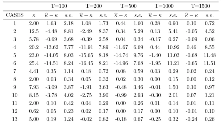
Table 1 gives simulation results for samples sizes T=100, 200, 500, 1000, 1500 and where b and its true standard errors (s:e) are obtained according to the estimator of Section 3 using a grid search. For computational purposes, the grid search of in the simulations is in the interval from 0.01 to
10 except in Cases 2 and 4-6, where since takes the larger values, the search interval has been extended from 0.01 until 30.
Table 1 : Without estimating the GARCH parameters
T=100 T=200 T=500 T=1000 T=1500 CASES b s:e: b s:e: b s:e: b s:e: b s:e:
1 2.00 1.63 2.18 1.08 1.73 0.44 1.60 0.28 0.90 0.10 0.72 2 12.5 -4.48 8.81 -2.49 8.37 0.34 5.29 0.13 5.41 -0.05 4.52 3 5.78 -0.69 3.68 -0.39 2.58 0.04 0.34 -0.17 0.27 -0.09 0.06 4 20.2 -13.62 7.77 -11.91 7.89 -11.67 6.69 0.44 10.92 0.46 8.55 5 23.0 -14.05 8.03 -15.65 8.18 -14.74 9.76 -1.40 11.03 -0.68 11.48 6 25.4 -14.51 8.24 -16.45 8.21 -14.96 7.68 -1.95 11.21 -0.65 11.51 7 4.41 0.35 1.14 0.18 0.72 0.08 0.59 0.03 0.29 0.02 0.24 8 2.00 0.03 0.34 0.05 0.32 0.02 0.30 0.00 0.15 0.00 0.12 9 7.93 -3.09 3.87 -1.91 3.63 -0.48 3.46 -0.01 1.50 0.10 0.97 10 8.15 -3.78 4.02 -2.75 3.90 -0.99 2.93 -0.30 2.01 0.07 1.21 11 2.00 0.10 0.42 0.04 0.29 0.00 0.26 0.01 0.14 0.01 0.11 12 0.62 0.05 0.23 0.02 0.17 0.00 0.17 0.00 0.10 -0.01 0.10 13 5.00 0.19 1.24 -0.02 0.82 -0.18 0.67 -0.25 0.32 -0.24 0.26
The second column of Table 1 provides the true values of . Some of them have been obtained from Groenendijk et al. (1995), Huisman et al (2001) and the rest have been simulated. Under the assumption
of "t N(0;1); ( ) =E[( "2t + ) =2
] 1can be expressed in terms of generalized Laguerre polynomials and the equation ( ) = 0 can be solved numerically.
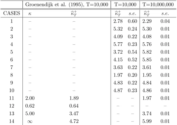
In order to compare our results in Table 1 with previous studies, Groenendijk et al. (1995) contain simulation results for ARCH type processes when 10,000 observations are available. Table 2 shows the values for our di¤erent ARCH processes (cases 11-13) and the true value of obtained from Groenendijk et al. (1995) with T=10,000: Comparing Tables 1 and 2, we obtain in Table 1 more precise point estimates than the Hill estimator of (i.e. b+
T) in Groenendijk et al. (1995) for the
true values of with even less than 1500 observations. Specially for large values of such as case 13, our estimator in Table 1 performs much better than the Hill estimator, since for = 5, we only obtain b+
T =3.74 even with 10,000,000 observations, while b = 5.19 even with T=100. Note again,
that the Hill estimator in Table 2 is shown for T=10,000 while in Table 1, we have much smaller sample sizes. Note also that in Table 2 we have extended the simulation results of Groenendijk et al. (1995) in cases 11, 13 and 14, since in those situations the Hill estimator does not provide a very precise estimate with 10,000 observations. Even with a sample size of 10,000,000, the Hill estimator o¤ers poor estimates for cases 13 and 14.
To get a comparison in the GARCH cases between Tables 1 and 2, we have extended again the simulation results of Groenendijk et al. (1995) of the Hill estimator of with m = 0:05T (m is the
number of order statistics) for our cases 1-10. Note that DuMouchel (1983) suggests that m= 0:1T
is a good rule, and m = 0:05T is a very common approach used in practice. We see again how in Table 2 for case 1, b+T is still far for the true = 2 even with 10,000 and 10,000,000 observations; while in Table 1, our estimator already provides a value close to 2 for T=500 and 1000. Note as well how the standard errors in Table 1 are also quite small for those sample sizes. Moreover, again for large values of such as cases 2 and 4-6, our estimator in Table 1 is able to provide estimates of that are much less biased than b+T in Table 2.
Case 3 provides a comparison with the results in Huisman et al (2001, Table 5, page 212). Using Huisman et al (2001) method, we get for sample sizes 100, 250, 500 and 1000 values equal to 7.04, 6.25, 5.88 and 5.56 respectively for the estimates of the true value of = 5:78: We see in Table 1 that our estimates are more precise in …nite samples than those in Huisman et al (2001).
Also, another important feature of our estimator is that if we compare Tables 1 and 2, specially for high values of ; the Hill estimator cannot provide estimates with small biases even with very large sample sizes. We have also computed the Hill’s (1975) estimator by choosing m with a mean squared error criterion by the bootstrap along the lines of Hill (2006), and the biases are not reduced in this case either. Our estimator in Table 1 provide values very close to the true ones in …nite samples. In case 14, when the true value of goes to 1 (see Groenendijk et al. (1995, Table 2, page 261)), the Hill estimator is able to reach a maximum estimated value of equal to 4.72 for 10,000 observations and of 5.99 for 10,000,000 observations. As we can see from Tables 1 and 2, specially for large values of generated by fat tails of the GARCH model, the Hill estimator is not able to produce a good estimate in …nite samples. In this simulation study we show that GARCH models can produce very large values of ; and specially in this case, the Hill estimator does not provide good …nite sample results. Kesten (1973) guarantees that our equation bT( ) = 0 should
Table 2 : Monte Carlo results for b+ T Groenendijk et al. (1995), T=10,000 T=10,000 T=10,000,000 CASES b+T b + T s:e: b + T s:e: 1 – – 2.78 0.60 2.29 0.04 2 – – 5.32 0.24 5.30 0.01 3 – – 4.09 0.22 4.08 0.01 4 – – 5.77 0.23 5.76 0.01 5 – – 3.72 0.54 5.82 0.01 6 – – 4.15 0.52 5.85 0.01 7 – – 3.63 0.22 3.61 0.01 8 – – 1.97 0.20 1.95 0.01 9 – – 4.83 0.22 4.84 0.01 10 – – 4.87 0.23 4.86 0.01 11 2.00 1.89 – – 1.97 0.01 12 0.62 0.64 – – – – 13 5.00 3.47 – – 3.74 0.01 14 1 4.72 – – 5.99 0.01
In the second column we provide again the true values of from Groenendijk et al. (1995).
5.1.2 The GARCH process is estimated
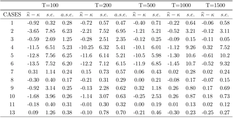
Table 3 shows the simulation results when the conditional heteroskedastic process is estimated. In the …rst, seventh and ninth cases, we have an IGARCH(1,1) and we know that = 2: Table 3 gives again simulation results for samples sizes T=100, 200, 500, 1000, 1500. b;true standard errors (s:e) and asymptotic standard errors (a:s:e:) from the previous Theorem in Section 4 are provided.
Kearns and Pagan (1997), note in their page 173 how “it seems unlikely that good estimates of a tail index could be made unless the sample size available is quite large, since the asymptotic theory shows that the convergence rate is …xed by m (the number of order statistics used in the computations) and this can only rise slowly with T”. Kearns and Pagan (1997) use around 29,000 observations to obtain a good estimate of the tail index when data is IGARCH(1,2); while Groe-nendijk et al. (1995) need 10,000 observations to get precise estimates of the tail index for an ARCH(1). We see in Table 3 how we can already obtain a very precise point estimate, with even much less than 1500 observations.
Case 3 provides a comparison with the results in Huisman et al (2001, Table 5). Again, our estimates have less bias than the ones in Huisman et al (2001). Note that one important remark is that Huisman et al (2001) method needs to remove correctly parametrically the heteroskedasticity by using a weighted-least squares estimation method, the same as in happens with our method that needs a correct speci…cation of the conditional variance equation.
Table 3: Estimating the GARCH parameters
T=100 T=200 T=500 T=1000 T=1500
CASES b s:e: a:s:e: b s:e: a:s:e: b s:e: b s:e: b s:e:
1 -0.92 0.32 0.28 -0.72 0.57 0.47 -0.40 0.71 -0.22 0.64 -0.06 0.58 2 -3.65 7.85 6.23 -2.21 7.52 6.95 -1.21 5.21 -0.52 3.21 -0.12 3.11 3 -0.59 2.69 1.25 -0.28 2.51 2.35 -0.12 0.25 -0.09 0.15 -0.11 0.05 4 -11.5 6.51 5.23 -10.25 6.32 5.41 -10.1 6.01 -1.12 9.26 0.32 7.52 5 -12.8 7.56 6.25 -11.6 6.14 5.21 -10.5 5.98 -1.30 10.6 -0.61 10.2 6 -13.5 7.52 6.20 -12.2 7.12 6.15 -11.9 6.85 -1.45 10.7 -0.52 9.32 7 0.31 1.14 0.24 0.15 0.73 0.57 0.06 0.43 0.02 0.28 0.02 0.24 8 -0.30 0.40 0.17 -0.21 0.31 0.29 0.00 0.21 -0.08 0.17 -0.07 0.15 9 -0.92 3.14 0.25 -0.13 2.28 0.62 0.32 1.18 0.26 0.80 0.17 0.69 10 -1.68 3.96 0.26 -1.14 3.07 0.63 -0.25 2.53 0.26 0.87 0.18 0.73 11 -0.18 0.40 0.31 -0.01 0.30 0.32 0.00 0.19 0.01 0.13 0.02 0.12 13 0.09 1.26 0.38 -0.10 0.78 0.70 -0.21 0.46 -0.30 0.23 -0.25 0.27
5.2
Application
One of the conclusions from the previous Monte Carlo results, is that our new estimator seems to have clear advantages compared with the traditional Hill estimator mainly when the true value of is large. We conduct now an empirical application to show the usefulness of our approach.
As Kearns and Pagan (1997) point out, there are many reasons why we want to have precise estimates of : For example, banks are interested in risk management and therefore, this relates to the probability of having either a large positive or negative realization of the random variables underlying the portfolios, i.e., computation of value at risk. Precise estimates of can also help us to discriminate between di¤erent probability models, and also, they can help us to …nd out how many moments of the data exist (see e.g., Loretan and Phillips (1994)). All this justi…es the need to concentrate our e¤orts in improving the estimation procedures of : We proceed now to apply our method to di¤erent economic time series data.
Jansen and de Vries (1991) analyzed the behavior of the returns of the daily S&P500, and they used the Hill estimator to …nd an estimate for the value. They analyzed the period 1962-1986. They were worried about a structural change at 1973, so they split the sample size 1962-1986 in two subperiods. The Hill estimate for the …rst subperiod (from 1962-1973) of for the lower tail equals 3.71 and is 3.65 for the second period 1973-1986 (See Table 3, page 22 of Jansen and de Vries (1991, page 22)). However, Jansen and de Vries (1991) ignore both the modeling of the conditional variance equation and the dynamics in the mean equation.
Kearns and Pagan (1997) stated that Jansen and de Vries (1991) are neglecting a GARCH(1,1) in the conditional variance by applying the Hill estimator. More recently, Linton and Mammen (2005,
page 806) analyzed the behavior of the daily S&P500 in the period 1955-2002, and they …nd that an AR(2)-GJR-GARCH(1,1) model is more adequate for these data. They use the standard GJR model proposed by Glosten, Jagannathan and Runkle (1993) where
yt = d+b1yt 1+b2yt 2+ ut z}|{" t t; (20a) 2 t = !+ u 2 t 1+ u 2 t 11fut 1 <0g+ 2t 1: (20b)
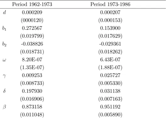
Our objective is to …nd out if by using explicitly an AR(2)-GJR-GARCH(1,1) model, we can get better estimates for :Note that, as discussed in Section 2, all the theory that we develop in Sections 2-4 is valid not only for the regular GARCH(1,1) model in the conditional variance, but also for a GJR-GARCH(1,1). Therefore, following Linton and Mammen (2005), we …tted also an AR(2)-GJR-GARCH(1,1) model for the two subperiods given in Jansen and de Vries (1991) as in (20a)-(20b), and Table 4 shows the results. Note that in both subperiods, when we check for neglected serial correlation both in the residuals and in the squares of the residuals, we cannot reject the null hypothesis of neglected serial correlation with the diagnostic tests of Ljung-Box (1978). This provides evidence that there is not dependence inb"t, and therefore, we can rely on the results of a strong-type
GJR-GARCH(1,1) model.
Table 4: Parametric estimation. Standard errors given in parenthesis Period 1962-1973 Period 1973-1986 d 0.000209 0.000207 (0000120) (0.000153) b1 0.272567 0.153900 (0.019799) (0.017629) b2 -0.038826 -0.029361 (0.018731) (0.018262) ! 8.20E-07 6.43E-07 (1.35E-07) (1.88E-07) 0.009253 0.025727 (0.008733) (0.005330) 0.197930 0.031138 (0.016906) (0.007163) 0.873158 0.951192 (0.011048) (0.005890)
From Table 4 and following Linton and Mammen (2005), the daily S&P500 can be better mod-eled by an AR(2)-GJR-GARCH(1,1) compared with the regular GARCH(1,1) of Kearns and Pagan (1997). Indeed we get statistically signi…cant results that there are asymmetric e¤ects in both sub-periods. Then, we proceed as follows: for each of the two subperiods, we …t an AR(2) process to
the daily returns of the S&P500. We take these residuals, and we …t a regular GJR-GARCH(1,1) to those residuals. Note that the fact of estimating …rst the mean equation and later to take the residuals to …t the conditional variance equation is a very common approach in empirical applications (see, e.g., Ball and Torous (1999, page 2349)).
Later we take the …tted standardized residuals (b"t) from the GJR-GARCH(1,1) and we …nd a
grid search of as in (8) where (see Straumann (2003))
b
At= b+b1fb"t<0g b"2t +b: (21)
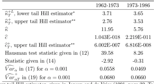
Our results are given in Table 5. In Table 5, we also report the results for the upper and lower tail Hill estimates, the statistics given in (12) and (14) and estimates of cde…ned in (3).
Table 5: Estimated values of for daily returns of S&P500 1962-1973 1973-1986
b+TL;lower tail Hill estimator 3.71 3.65 b+T; upper tail Hill estimator 2.76 3.53
b 11.95 5.76
b
c 1.043E-018 2.219E-011
b
c+T; upper tail Hill estimator 6.002E-007 6.816E-008 Hausman test statistic given in (12) 39.58 8.26 Statistic given in (14) -2.92 -0.31
d
V ar in (17) for = 0:001 0.0558 0.0469
d
V ar+T in (19) for = 0:001 0.0680 0.0660
Lower tail Hill estimator, given in Jansen and de Vries (1991, page 22, Table 3) We usem = 0:05T.
We get a value ofb that equals 11.95 from the grid search (taken in the interval 0.01 and 30) for the period 1962-1973. So, in this case, the estimated value of through the grid search (taking into account the AR(2)-GJR-GARCH(1,1) structure) is much larger than the estimated value of that is obtained through the Hill estimator without having into account the AR(2)-GJR-GARCH(1,1) (see Jansen and De Vries (1991, Table 3 in page 22)). However when we compute the Hausman test statistic given in (12), we obtain a clear rejection that b produces a consistent estimate of :
If we apply the same procedure for the second subperiod, we get an estimated value of equal to 5.76. So, we get a much higher value for than Jansen and de Vries (1991) with the Hill estimator. This is in accordance to the Monte Carlo results that we got in the previous section, where the Hill estimator seems to have large biases for large values of , while the estimator through the grid search is able to reduce those biases in this case. We therefore …nd much more evidence of a structural break than Jansen and de Vries (1991) in 1973 for the daily S&P500, when we take into account explicitly an AR(2)-GJR-GARCH(1,1) model as Linton and Mammen (2005) for the estimation of
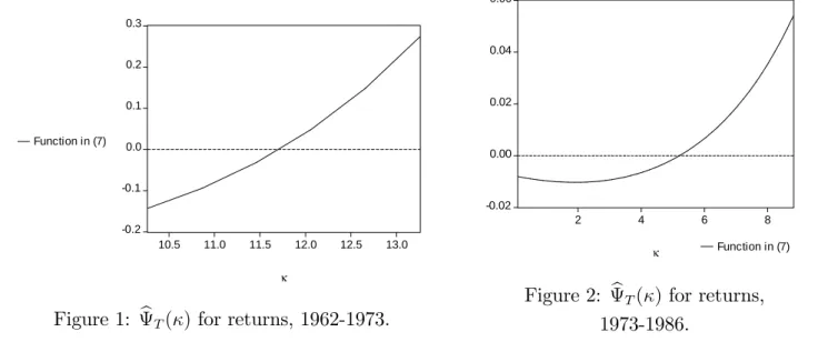
throughb. However, when we use the Hausman test statistic in (12), we reject the null hypothesis that bproduces a consistent estimate of :Therefore, in Table 5, we conclude that the Hill estimator is preferred to b in both subperiods. Moreover, there is statistically evidence through (14) that we reject the null hypothesis that the upper and lower tails are equal in the …rst time period although not in the second one. Figures 1 and 2 plot the values of bT( )in (8) as a function of for the two
subperiods. -0.2 -0.1 0.0 0.1 0.2 0.3 10.5 11.0 11.5 12.0 12.5 13.0 κ Function in (7)
Figure 1: bT( )for returns, 1962-1973.
-0.02 0.00 0.02 0.04 0.06 2 4 6 8 κ Function in (7)
Figure 2: bT( ) for returns,
1973-1986.
Table 5 also reports the estimates of cin (3) both with our proposed estimator(bc)and with the Hill estimator bc+T :
In Table 5, for the period 1962-1973 we obtain a value of bequal to 11.95 but the Hausman type test rejects that provides a consistent estimator, and the Hill estimator bc+T is clearly preferable to be used for value at risk purposes. For the period 1973-1986, although we obtain a very similar point estimate for c both withbcand bc+T; in this case, the Hausman type test advises the use ofb+T instead of b; and therefore, we prefer V ard+T instead of V ard in both time periods. Table 5 also provides
d
V ar+T and V ard in both time periods for = 0:001 as an example. Another important remark is that for example in Figure 2 we have started the search of at 0.01 and we do not evaluate the function at 0. That is why the function in Figure 2 does not show clearly graphically that b(0) = 0:
The same happens for the rest of the pictures.
In order to show more evidence of the di¤erent estimates of that we can obtain with di¤erent estimation procedures and that b can be useful in some applications, we proceed now to analyze di¤erent time series of oil prices. We obtained the data from the Oil Price Information Service (OPIS)1. Petroleum product prices from OPIS have been the focus of attention of many authors in
the literature, such as Slade (1986), Pinkse, Slade and Brett (2002) and Doyle and Samphantharak
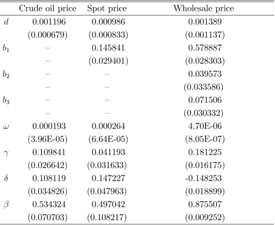
(2005). We have daily data (no weekends) from 12/21/1998 until 01/30/2004 of the prices on crude oil price (crude), spot prices of gasoline (spot), and wholesale prices of gasoline (wholesale). We …rst compute the returns on each of the prices as the …rst di¤erence of the logarithms, and the three returns can be shown to reject the null hypothesis of a unit root with an Augmented Dickey Fuller (1979) and Phillips and Perron (1988) tests. Later we …t a GJR-GARCH(1,1) model with a constant in the mean equation for the returns of crude, an AR(1) with a constant in the mean equation and a GJR-GARCH(1,1) for the returns of the spot prices and an AR(3) with a constant in the mean equation and a GJR-GARCH(1,1) for the returns on the wholesale of prices of gasoline. These are the models that allow not to reject the null hypothesis of neglected serial correlation both in the residuals and in the squares of the residuals with the diagnostic tests of Ljung-Box (1978) for the three time series. This provides evidence that we are in the presence of strong-type GJR-GARCH(1,1) models in the three cases. Table 6 shows the estimates of the previous models following again the notation as in (20a)-(20b), and whereb3 corresponds to the coe¢ cient of the third lag ofyt in the mean equation.
Later, we proceed as before, and we …rst …t, for example for the returns on spot prices of gasoline, an AR(1) and a constant in the mean equation, we take the residuals, and we …t a GJR-GARCH(1,1). We take the standardized residuals and we …nd a grid search of as in (21). Table 7 shows the results both when we use the Hill estimator (with the upper and lower tails) and when we use the grid search.
Table 6: Parametric estimation. Standard errors given in parenthesis Crude oil price Spot price Wholesale price
d 0.001196 0.000986 0.001389 (0.000679) (0.000833) (0.001137) b1 – 0.145841 0.578887 – (0.029401) (0.028303) b2 – – 0.039573 – – (0.033586) b3 – – 0.071506 – – (0.030332) ! 0.000193 0.000264 4.70E-06 (3.96E-05) (6.64E-05) (8.05E-07)
0.109841 0.041193 0.181225 (0.026642) (0.031633) (0.016175) 0.108119 0.147227 -0.148253 (0.034826) (0.047963) (0.018899) 0.534324 0.497042 0.875507 (0.070703) (0.108217) (0.009252)
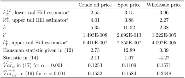
Table 7: Estimated values of for daily returns of oil prices
Crude oil price Spot price Wholesale price
b+TL; lower tail Hill estimator 2.55 3.15 3.96 b+T; upper tail Hill estimator 4.01 3.88 2.27
b 5.35 10.02 2.38
b
c 1.493E-008 2.692E-013 1.222E-005
b
c+T; upper tail Hill estimator 5.410E-007 7.855E-007 4.097E-005 Hausman statistic given in (12) 2.73 12.89 0.39 Statistic in (14) 2.11 1.07 -4.27 d V ar in (17) for = 0:001 0.1253 0.1109 0.1571 d V ar+T in (19) for = 0:001 0.1532 0.1584 0.2448 We usem = 0:05T.
One interesting remark in Table 7 is thatb+L
T is larger thanb
+
T for wholesale price (as expected);
however, this is not true for crude oil price and spot price. This fact is in accordance with for example Table 2 in Jansen and de Vries (1991), where they also …nd in 3 of their 10 stocks that b+L
T is smaller
than b+
T:This again con…rms the existence of large biases in the Hill estimator that can produce that
in practice, we can get estimates of the Pareto exponent parameters where the lower tail is much thicker than the upper tail.
Again, Table 7 con…rms that the Hill estimator tends to produce smaller values for the estimated than through the grid search. This is a …nding that we get repeatedly both in the Monte Carlo results in the previous Section and in the applications. Figures 3 and 4 also show, for the cases of crude oil price and spot price, the values of bT( )in (8) as a function of :Note that the grid search
has been carried out in the interval [0:01;30]. Figure 3 shows how bT( ) equals zero for b = 5:35:
However, Figure 4 shows how for spot price, the value of for which the objective function equals 0 is 10.02. Figure 5 corresponds to wholesale price, where the values of have been re-scaled to show more clearly the point where the objective function equals 0.
-2 0 2 4 6 8 10 12 2 4 6 8 κ Function in (7)
Figure 3: bT( ) for crude oil price.
-5 0 5 10 15 20 25 30 8 10 12 14 16 κ Function in (7)
Figure 4: bT( ) for spot price.
-0.02 0.00 0.02 0.04 0.06 0.08 1.5 2.0 2.5 3.0 3.5 κ Function in (7)
Figure 5: bT( ) for wholesale price.
Table 7 also reports the results of the Hausman type tests of Section 4. The analysis of the Hausman test in (12) shows that for spot price we clearly reject the null hypothesis that b provides a consistent estimator, so in this case we should use the Hill estimator. For crude oil price, the test rejects at 1% (critical value 2.58) and 10% (critical value 1.64) although it is not a very clear rejection at 1% (2.73 is not very far from the critical value of 2.58). And for wholesale price, the test cannot reject that b provides a consistent estimator.
The analysis of the test for equal tails in (14), reveals that we cannot reject that null hypothesis for crude oil price and for spot price. Therefore, there are no gains in computing an upper tail and a lower tail through the Hill estimator in these two cases.
Therefore, the conclusion is that for crude oil price there is some statistical evidence of the advantage of b to produce a less biased estimate of instead of using b+
T; and as obtained through
upper tail from the Hill estimator (4.01). The Hausman type test in (12) does not provide a very clear rejection at 1% signi…cance level, and also (14) reveals that there is not statistically signi…cant evidence against equal lower and upper tails at 1%. For spot price there is statistical evidence that the Hill estimator should be clearly used. And for wholesale price, there is evidence that bprovides a consistent estimate of that is higher than b+T (and therefore b is clearly preferred to b+T in this case). Moreover, there is also evidence that b+TL is statistically signi…cantly di¤erent from b+T for wholesale price, and therefore both b and b+TL should be used in this case.
Finally, both bc and bc+T show very similar estimates of c. Since for both crude oil price and wholesale price there is evidence of the advantages of usingbversusb+T;for these two series we prefer the measure of value at risk given by (17) instead of (19), while for the case of spot price, (19) is clearly superior. Table 7 also reports the values of V ard and V ard+T for example for = 0:001. For crude oil price, and wholesale price (where we prefer our new measure V ard versus V ard+T), it is clear that V ard produces a di¤erent result thanV ard+T.
6
Conclusion
We propose a method of estimating a Pareto tail thickness parameter and gave its corresponding distributional theory in the context of the GJR-GARCH model (extending the results of St¼aric¼a and Pictet (1997) and Berkes, Horváth and Kokoszka (2003)). Provided the conditional variance is correctly speci…ed, the resulting estimator of tail thickness converges at rate pT to a normal distribution (where T is the sample size). This is much faster than the convergence rate of the Hill estimator, since that procedure only uses a vanishing fraction of the sample. However, our asymptotics are predicated on the correctness of the model for conditional variance at the least, and this may be questionable. In the case where the model does not hold it would be nice to use the new estimator in a ‘prewhitening’ strategy as has been done in other literatures, namely spectral density estimation, see Linton and Xiao (2002) for a recent discussion, but we have not been directly able to carry this idea over successfully to estimating Pareto tails. One related approach that might achieve similar objectives is due to Fan and Ullah (1999), which involves combining our estimator with the Hill estimator sob =bb+T+(1 b)b;where the weighting sequencebis data dependent and satis…es: b !p 0 when the GJR-GARCH model is true and b !p 1 otherwise. It can be expected that this procedure can be madepT consistent when the GJR-GARCH model is true but still retains consistency otherwise. We also propose a new estimator in the literature of Value at Risk based on the tail thickness estimator. The new estimator can be used as a speci…cation test of the GARCH model, and we propose a Hausman type test to do this.
We …nd quite heavy tails for the daily stock return data and the various oil return series, there being some discrepancies between the Hill estimator and our GJR-GARCH-based estimator. In some cases, these di¤erences are statistically signi…cant. It is interesting that in some cases, the
GJR-GARCH model-based estimator yields heavier tails than the Hill estimator, although the opposite also happens. In any case, the tail thicknesses are quite substantial and their precise numerical value has a big impact on the implied Value at Risk, which makes it very important to have the most precise estimates possible. We hope that our methodology can contribute to that objective.
7
Appendix
Proof of Theorem. Consider the infeasible estimator e that is any solution to
T(e) =op(T 1=2); T( ) = 1 T T X t=1 At=2 1:
This estimator is a standard (parametric) …rst order condition estimator and its properties follow by standard arguments. We …rst show consistency. First, we have by Andrews (1987) ULLN
sup 2Kj T( ) ( )j=op(1); (22) because 0( ) = E[A =2 t ln(At)]=2 < 1 and E[sup 0:j 0 j jA 0=2 t ln(At)j] E[jA ( + )=2 t j] < 1 for
some >0: Then by the uniqueness of ; we havee!p :
Furthermore, 0 = T(e) = T( 0) + 0T( )(e 0); wherej j je 0jand 0T( ) = (2T) 1 PT t=1A =2
t ln(At):By the Andrews ULLN again we have
0 T( ) P ! 12EhAt=2ln(At) i =M;
where M is bounded away from zero and in…nity, since E[sup 0:j 0 j j 00( )j] =
E[sup 0:j 0 j jA
=2
t fln(At)g2j]<1: Also, by the CLT for stationary mixing processes we have
p T T( 0) = 1 p T T X t=1 h A 0=2 t E A 0=2 t i D !N(0; V1) V1 = 1 X j= 1 cov( t; t+j); where t=A 0=2
t 1is mean zero. Therefore,
p T(e 0) = M 1 p T T( 0) +op(1) D !N(0; M 2V1):
We now turn to the feasible estimator. To establish consistency of b it su¢ ces to show that
sup
2K
For any we can write T( ; ) =T 1PTt=1At=2( ): Then we decompose
T( ; ) = T( ; 0) + T( ; ) T( ; 0)
= T( ) +E[ T( ; )] E[ T( ; 0)] + T( ; );
where T( ; ) = T( ; ) E[ T( ; )] f T( ; 0) E[ T( ; 0)]g: The process T( ; ) is
sto-chastically equicontinuous in in the sense that
sup
2K
sup
k 0k T
j T( ; )j=op(1); (24)
where T is a sequence of positive numbers tending to zero such that Pr[jj 0jj T]!1; such a
sequence is guaranteed by the consistency ofb:The result (24) follows by standard empirical process theory since the parameters ; 2 enter in a nice smooth way, while the parameters 1 enters as shifts
inside an indicator function, see for example CLV (2003). Then it follows that with probability tending to one sup 2K bT( ) T( ) T sup k 0k T sup 2K @E[ T( ; )] @ @E[ T( ; 0)] @ +op(1) =op(1):
It follows that (23) holds and hence b is consistent.
To establish asymptotic normality ofb we Taylor expand to …rst order
0 = bT(b) = bT( 0) + b0T( )(b 0); (25)
where is an intermediate value. It follows from the consistency property that there exists a sequence
T !0with Pr[jb j T;
p
Tjj 0jj T]!1: For this sequence we obtain
sup :j 0j T sup :jj 0jj T j 0T( ; ) 0( ; )j = op(1) p T sup :j 0j T sup :jj 0jj T j T( ; )j = op(1) sup :j 0j T sup :jj 0jj T @E[ T( ; )] @ @ ( ; ) @ = op(1);
by standard empirical process results. From this it follows that:
bT( 0) = T( 0) + @E[ T( ; 0)] @ > (b 0) +op(T 1=2) b0 T( ) = 0( 0) +op(1):
In conclusion we obtain the expansion
p T(b 0) = M 1 " p T T( 0) + @ ( 0) @ > 1 p T T X t=1 t # +op(1): (26)
The central limit theorem follows from the mixing assumption.
Note that"t( ) is di¤erentiable in 2 = (!; ; ; )>;and we obtain:
@ T( ; ) @ 2 = 1 T T X t=1 @At=2( ) @ 2 = 2 1 T T X t=1 @At @ 2 ( )A(t 2)=2( ); where: @At @! ( ) = 2 ( + 1fut( 1)<0g) @"t @!( )"t( ) = ( + 1fut( 1)<0g) ut( 1)"t( ) 3 t( ) @ 2 t @! ( ); (27) @At @ ( ) = 2 ( + 1fut( 1)<0g) @"t @ ( )"t( ) + 1 = ( + 1fut( 1)<0g) ut( 1)"t( ) 3 t( ) @ 2t @ ( ) + 1; (28) @At @ ( ) = 2 ( + 1fut( 1)<0g) @"t @ ( )"t( ) +" 2 t( ) = ( + 1fut( 1)<0g) ut( 1)"t( ) 3 t( ) @ 2 t @ ( ) +" 2 t( ); (29) @At @ ( ) = 2 ( + 1fut( 1)<0g) @"t @ ( )"t( ) +" 2 t( ) (1fut( 1)<0g) = ( + 1fut( 1)<0g) ut( 1)"t( ) 3 t( ) @ 2 t @ ( ) +" 2 t( ) (1fut( 1)<0g); (30) where @ 2 t @! ( ) = 1 + @ 2t 1 @! ( ) = "t 1 X i=0 i+ t@ 20 @! # ; @ 2t @ ( ) = u 2 t 1( 1) + @ 2 t 1 @ ( ) = "t 1 X i=0 i u2t i 1+ t@ 2 0 @ # ; @ 2 t @ ( ) = u 2 t 1( 1)1fut 1( 1)<0g+ @ 2 t 1 @ ( ); @ 2 t @ ( ) = 2 t 1( ) + @ 2t 1 @ ( ) = "t 1 X i=0 i 2 t i 1( ) + t@ 20 @ # :
References
[1] Andrews, D.W.K., (1987), Consistency in nonlinear econometric models: A generic uniform law of large numbers,Econometrica 55, 1465-1471.
[2] Andrews, D.W.K., (1991), Heteroskedasticity and Autocorrelation Consistent Covariance Ma-trix Estimation.Econometrica 59, 817-858.
[3] Ball, C. A. and W. N. Torous (1999), The Stochastic Volatility of Short-Term Interest Rates: Some International Evidence,The Journal of Finance 54, 6, 2339-2359.
[4] Berkes, I., L. Horváth and P. Kokoszka (2003), Estimation of the Maximal Moment Exponent of a GARCH(1,1) Sequence, Econometric Theory 19, 565-586.
[5] Bickel, P. J., Klaassen, C. A. J., Ritov, Y. and J. A. Wellner (1993),E¢ cient and adaptive esti-mation for semiparametric models. The John Hopkins University Press, Baltimore and London. [6] Bollerslev, T. (1986), Generalized Autoregressive Conditional Heteroscedasticity, Journal of
Econometrics 31, 307-327.
[7] Borkovec, M. (2000), Extremal Behavior of the Autoregressive Process with ARCH(1) Errors,
Stochastic Processes and their Applications 85, 2, 189-207.
[8] Borkovec, M. and C. Klüppellberg (2001), The Tail of the Stationary Distribution of an Autore-gressive Process with ARCH(1) Errors,Annals of Applied Probability 11, 4, 1220-1241.
[9] Breiman, L. (1965), On Some Limit Theorems Similar to the Arc Sin Law,Theory of Probability and Its Applications 10, 323-331.
[10] Carrasco, M. and Chen, X. (2002), Mixing and Moment Properties of Various GARCH and Stochastic Volatility Models,Econometric Theory, 18, 17-39.
[11] Chen, X., O. Linton and I. Van Keilegom (2003). Estimation of Semiparametric Models when the Criterion is not Smooth,Econometrica 71, 1591-1608.
[12] Danielsson, J. and C.G. de Vries (2000). Value-at Risk and Extreme Returns. http://www.riskresearch.org/
[13] Dekkers, A., J. Einmahl and L. De Haan (1989), A Moment Estimator for the Index of an Extreme-value Distribution,Annals of Statistics 17, 1833-1855.
[14] Dickey, D. A. and W. A. Fuller (1979), Distribution of the Estimators for Autoregressive Time Series with a Unit Root,Journal of the American Statistical Association 74, 427-431.
[15] Doyle, J. J. Jr. and K. Samphantharak (2005), $2.00 Gas! Studying the E¤ects of Gas Tax Moratorium, Working Paper, MIT Center for Energy and Environmental Policy Research 05-017.
[16] Drees, H. (2000), Weighted Approximations of Tail Processes for mixing random variables,
[17] Drees, H. (2003), Extreme Quantile Estimation for Dependent Data with Applications to Fi-nance,Bernouilli 9, 4, 617-657.
[18] Drost, F.C., and T.E. Nijman (1993), Temporal Aggregation of GARCH Processes, Economet-rica 61, 909-927.
[19] DuMouchel, W. H. (1983), Estimating the Stable Index in Order to Measure Tail Thickness: A Critique,Annals of Statistics 11, 1019-1031.
[20] Embrechts, P., C. Klüppellberg and T. Mikosch (1998), Modelling Extremal Events for Insurance and Finance, Springer, New York.
[21] Engle, R. F. (1982), Autoregressive Conditional Heteroscedasticity with Estimates of the Vari-ance of United Kingdom In‡ation,Econometrica 50, 987-1007.
[22] Fama, E. F. (1965), The Behavior of Stock Market Prices, Journal of Business 38, 34-105. [23] Fama, E. F. (1976), Foundations of Finance, New York: Basic Books.
[24] Fan, Y., and A. Ullah (1999). Asymptotic normality of a combined regression estimator. Journal of Multivariate Analysis 71, 191-240.
[25] Gabaix, X., P. Gopikrishnan, V. Plerou and H. E. Stanley (2006), Institutional Investors and Stock Market Volatility,Quarterly Journal of Economics, 461-504.
[26] Gabaix, X. and R. Ibragimov (2006), Rank-1/2: A Simple Way to Improve the OLS Estimation of Tail Exponents, Harvard Institute of Economic Research Discussion Paper No. 2106.
[27] Glosten, L. R., R. Jagannathan and D. E. Runkle (1993), On the Relationship Between the Expected Value and the Volatility of the Nominal Excess Returns on Stocks,Journal of Finance
48, 1779-1801.
[28] Groenendijk, P. A., A. Lucas and C. G. de Vries (1995), A Note on the Relationship Between GARCH and Symmetric Stable Processes, Journal of Empirical Finance 2, 253-264.
[29] Hill, B. M. (1975), A Simple General Approach to Inference about the Tail of a Distribution,
Annals of Statistics 3, 1163-1174.
[30] Hill, J. B. (2006), On tail index estimation for dependent, heterogenous data, Working Paper, Florida International University.
[31] Hols, M. C. A. B. and C. G. de Vries (1991), The Limiting Distribution of Extremal Exchange Rate Returns,Journal of Applied Econometrics 6, 287-302.
[32] Hsing, T. (1991), On Tail Index Estimation using Dependent Data, Annals of Statistics 19, 3, 1547-1569.
[33] Huisman, R., K. G. Koedijk, C. J. M. Kool and F. Palm (2001), Tail-Index Estimates in Small Samples, Journal of Business and Economic Statistics 19, 2, 208-216.
[34] Jansen, D. W. and C. G. de Vries (1991), On the Frequency of Large Stock Returns: Putting Booms and Busts into Perspective, Review of Economics and Statistics 73, 18-24.
[35] Jensen, S. T. and A. Rahbek (2004a), Asymptotic Normality of the QML Estimator of ARCH in the Nonstationary Case,Econometrica, 72, 2, 641-646.
[36] Jensen, S. T. and A. Rahbek (2004b), Asymptotic Inference for Nonstationary GARCH, Econo-metric Theory 20, 6, 1203-1226.
[37] Kearns, P. and A. Pagan (1997), Estimating the Density Tail Index for Financial Time Series,
Review of Economics and Statistics 79, 2, 171-175.
[38] Kesten, H. (1973), Random Di¤erence Equations and Renewal Theory for Products of Random Matrices,Acta Mathematica 131, 207-48.
[39] Koedijk, K. G., M. M. Schafgans and C. G. de Vries (1990), The Tail Index of Exchange Rate Returns,Journal of International Economics 29, 93-108.
[40] Lange, T., A. Rahbek and S. T. Jensen (2006), Estimation and Asymptotic Inference in the First Order AR-ARCH Model, Preprint no.4, Department of Mathematical Sciences, University of Copenhagen.
[41] Lee, S.-W. and B. E. Hansen (1994), Asymptotic Theory for the GARCH(1,1) Quasi-Maximum Likelihood Estimator, Econometric Theory 10, 29-52.
[42] Ling, S. and M. McAleer (2003), Asymptotic Theory for a Vector ARMA-GARCH Model,
Econometric Theory 19, 280-310.
[43] Linton, O. (1993), Adaptive estimation in ARCH models, Econometric Theory 9, 539-569. [44] Linton, O. and E. Mammen (2005), Estimating Semiparametric ARCH(1) Models by Kernel
Smoothing Methods,Econometrica 73, 3, 771-836.
[45] Linton, O., J. Pan, and H. Wang (2007), Estimation for a non-stationary semi-strong GARCH model with heavy tailed errors. Manuscript, LSE.
[46] Linton, O. and Z. Xiao (2002). A Nonparametric Prewhitened Covariance Estimator, Journal of Time Series Analysis 23, 215-250.
[47] Ljung, G. M. and G. E. P. Box (1978), On a Measure of a Lack of Fit in Time Series Models,
Biometrika 65, 297-303.
[48] Loretan, M. and P. C. B. Phillips (1994), Testing the Covariance Stationarity of Heavy-Tailed Time Series: An Overview of the Theory with Applications to Several Financial Time Series,
Journal of Empirical Finance 1, 211-248.
[49] Mandelbrot, B. (1963), The Variation of Certain Speculative Prices, Journal of Business 36, 392-417.
[50] Markowitz, H. (1991), Foundations of Portfolio Theory, The Journal of Finance 7, 469-477. [51] McNeil, A.J., R. Frey, and P. Embrechts (2005). Quantitative Risk Management. Princeton
University Press, Princeton.
[52] Meitz, M. and P. Saikkonen (2006). Stability of nonlinear AR-GARCH Models. SSE Working paper no. 632.
[53] Mikosch, T. and C. St¼aric¼a (2000), Limit Theory for the Sample Autocorrelations and Extremes of a GARCH(1,1) Process, Annals of Statistics 28, 5, 1427-1451.
[54] Nelson, D.B. (1990), Stationarity and Persistence in the GARCH(1,1) model, Econometric The-ory 6, 318-34.
[55] Osborne, M. F. M. (1959), Brownian Motion in the Stock Market, Operation Research 7, 145-173.
[56] Peng, L., and Q. Yao (2003), Least absolute deviations estimation for ARCH and GARCH models, Biometrika 90, 967-975.
[57] Phillips, P. C. B. and P. Perron (1988), Testing for a Unit Root in Time Series Regression,
Biometrika 75, 335-346.
[58] Pinkse, J., M. E. Slade and C. Brett (2002), Spatial Price Competition: A Semiparametric Approach,Econometrica 70, 3, 1111-1153.
[59] Resnick, S. and C. St¼aric¼a (1997), Asymptotic Behavior of the Hill’s Estimator for Autoregressive Data,Stochastic Models 13, 4, 703-721.
[60] Resnick, S. and C. St¼aric¼a (1998), Tail Estimation for Dependent Data, Annals of Applied Probability 8, 4, 1156-1183.
[61] Rosenblatt, M. (1956), A central limit theorem and strong mixing conditions, Proc. Nat. Acad. Sci.4, 43-47.
[62] Slade, M. E. (1986), Exogeneity Tests of Market Boundaries Applied to Petroleum Products,
The Journal of Industrial Economics 34, 3, 291-303.
[63] St¼aric¼a, C. (1998), On the Tail Empirical Process for Stochastic Di¤erence Equations, Working paper.
[64] St¼aric¼a, C. and O. Pictet (1997), The tales the tails of GARCH processes tell. Unpublished Working paper.
[65] Straumann, D., (2003). Estimation in Conditionally Heteroscedastic Time Series Models. PhD Thesis, University of Copenhagen.
[66] Straumann, D. and T. Mikosch (2006), Quasi-Maximum-Likelihood Estimation in Conditionally Heteroscedastic Time Series: A Stochastic Recurrence Equations Approach, The Annals of Statistics 34, 5, 2449-2495.
[67] Wagner, N. and T. A. Marsh (2005), Measuring Tail Thickness under GARCH and an Applica-tion to Extreme Exchange Rate Changes, Journal of Empirical Finance 12, 165-185.