2008/64
■
Nonnegative factorization
and the maximum edge biclique problem
CORE
Voie du Roman Pays 34
B-1348 Louvain-la-Neuve, Belgium. Tel (32 10) 47 43 04
Fax (32 10) 47 43 01
E-mail: [email protected] http://www.uclouvain.be/en-44508.html
CORE DISCUSSION PAPER 2008/64
Nonnegative factorization and the maximum edge biclique probem Nicolas GILLIS 1 and François GLINEUR2
November 2008
Abstract
Nonnegative Matrix Factorization (NMF) is a data analysis technique which allows compression and interpretation of nonnegative data. NMF became widely studied after the publication of the seminal paper by Lee and Seung (Learning the Parts of Objects by Nonnegative Matrix Factorization, Nature, 1999, vol. 401, pp. 788--791), which introduced an algorithm based on Multiplicative Updates (MU). More recently, another class of methods called Hierarchical Alternating Least Squares (HALS) was introduced that seems to be much more efficient in practice.
In this paper, we consider the problem of approximating a not necessarily nonnegative matrix with the product of two nonnegative matrices, which we refer to as Nonnegative Factorization~(NF)~; this is the subproblem that HALS methods implicitly try to solve at each iteration. We prove that NF is NP-hard for any fixed factorization rank, using a reduction to the maximum edge biclique problem.
We also generalize the multiplicative updates to NF, which allows us to shed some light on the differences between the MU and HALS algorithms for NMF and give an explanation for the better performance of HALS. Finally, we link stationary points of NF with feasible solutions of the biclique problem to obtain a new type of biclique finding algorithm (based on MU) whose iterations have an algorithmic complexity proportional to the number of edges in the graph, and show that it performs better than comparable existing methods.
Keywords: nonnegative matrix factorization, nonnegative factorization, complexity, multiplicative updates, hierarchical alternating least squares, maximum edge biclique.
1 CORE, Université catholique de Louvain, Belgium. E-mail: [email protected] 2CORE, Université catholique de Louvain, Belgium. E-mail: [email protected].
We thank Pr. Paul Van Dooren and Pr. Laurence Wolsey for helpful discussions and advice. The first author is a research fellow of the Fonds de la Recherche Scientifique (F.R.S.-FNRS). The second one is also member of ECORE, the newly created association between CORE and ECARES.
This paper presents research results of the Belgian Program on Interuniversity Poles of Attraction initiated by the Belgian State, Prime Minister's Office, Science Policy Programming. The scientific responsibility is assumed by the authors.
1
Introduction
(Approximate) Nonnegative Matrix Factorization (NMF) is the problem of approximating a given nonnegative matrix by the product of two low-rank nonnegative matrices: given a matrixM ≥0, one has to compute two low-rank matricesV, W ≥0 such that
M ≈V W . (1.1)
This problem was first introduced in 1994 by Paatero and Tapper [25], and more recently received a considerable interest after the publication of two papers by Lee and Seung [21, 22]. It is now well established that NMF is useful in the framework of compression and interpretation of nonnegative data ; it has for example been applied in analysis of image databases, text mining, interpretation of spectra, computational biology and many other applications (see e.g. [2, 9, 11] and references therein). How can one interpret the outcome of a NMF? Assume each columnM:j of matrixM represents an element of a data set: expression (1.1) can be equivalently written as
M:j ≈
X
k
V:kWkj, ∀j (1.2)
where each element M:j is decomposed into a nonnegative linear combination (with weights Wkj) of nonnegative basis elements ({V:k}, the columns of V). Nonnegativity of V allows interpretation of the basis elements in the same way as the original nonnegative elements in M, which is crucial in applications where the nonnegativity property is a requirement (e.g. where elements are images described by pixel intensities or texts represented by vectors of word counts). Moreover, nonnegativity of the weight matrix W corresponds to an essentially additive reconstruction which leads to a part-based representation: basis elements will represent similar parts of the columns of M. Sparsity is another important consideration: finding sparse factors improves compression and leads to a better part-based representation of the data [19].
We start this paper with a brief introduction to the NMF problem: Section 2 recalls existing complexity results, introduces two well-known classes of methods: multiplicative updates [22] and hierarchical alternating least squares [6] and proposes a simple modification to guarantee their conver-gence. The central problem studied in this paper, Nonnegative Factorization (NF), is a generalization of NMF where the matrix to be approximated with the product of two low-rank nonnegative matrices is not necessarily nonnegative. NF is introduced in Section 3, where it is shown to be NP-hard for any given factorization rank, using a reduction to the problem of finding a maximum edge biclique. Stationary points of the NF problem used in that reduction are also studied. This section ends with a generalization of the NMF multiplicative updates rules to the NF problem and a proof of their convergence. This allows us to shed new light on the standard multiplicative updates for NMF: a new interpretation is given in Section 4, which explains the relatively poor performance of these methods and hints at possible improvements. Finally, Section 5 introduces a new type of biclique finding algo-rithm that relies on the application of multiplicative updates to the equivalent NF problem considered earlier. This algorithm only requires a number of operations proportional to the number of edges of the graph per iteration, and is shown to perform well when compared to existing methods.
2
Nonnegative Matrix Factorization (NMF)
Given a matrixM ∈Rm×n+ and an integerr∈N0, theNMF optimization problem using the Frobenius norm is defined as min V∈Rm×r,W∈Rr×n ||M −V W||2F = X i,j (M−V W)2ij such thatV, W ≥0 (NMF)
Rm×n denotes the set of real matrices of dimensionm×n;Rm×n+ the set of nonnegative matrices i.e. Rm×n with every entry nonnegative, and0 the zero matrix of appropriate dimensions.
A wide range of algorithms have been proposed to find approximate solutions for this problem (see e.g. [2, 4, 6, 7, 10, 11, 13, 24]). Most of them use the fact that although problem (NMF) is not convex, its objective function is convex separately in each of the two factorsV andW (which implies that finding the optimal factorV corresponding to a fixed factorW reduces to a convex optimization problem, and vice-versa), and try to find good approximate solutions by using alternating minimization schemes. For instance, Nonnegative Least Squares (NNLS) algorithms can be used to minimize (exactly) the cost function alternatively over factorsV andW (see e.g. [5, 20]).
Actually, there exist other partitions of the variables that preserve convexity of the alternating minimization subproblems: since the cost function can be rewritten as ||M −Pr
i=1V:iWi:||F, it is clearly convex as long as variables do not include simultaneously an element of a column of V and an element of the corresponding row of W (i.e. Vki and Wil for the same index i). Therefore, given a subset of indexes K ⊆R={1,2, . . . , r}, (NMF) is clearly convex for both the following subsets of variables PK = n V:i i∈K o ∪ nWj: j∈R\K o
and its complement
QK = n V:i i∈R\K o ∪ nWj: j∈K o .
However, the convexity is lost as soon as one column of V (V:i) and the corresponding row of W (Wi:) are optimized simultaneously, so that the corresponding minimization subproblem can no longer be efficiently solved up to global optimality.
2.1 Complexity
Vavasis studies in [30] the algorithmic complexity of the NMF optimization problem; more specifically, he proves that the following problem, calledExact Nonnegative Matrix Factorization1, is NP-hard:
(Exact NMF) Given a nonnegative matrixM ≥0 of rankk, find, if possible, two nonneg-ative factorsV ≥0 andW ≥0 of rankk such thatM =V W.
The NMF optimization problem is therefore also NP-hard, since when the rankr is equal to the rank kof the matrixM, any optimal solution to the NMF optimization problem can be used to answer the Exact NMF problem (the answer being positive if and only if the optimal objective value of the NMF optimization problem is equal to zero).
The NP-hardness proof for exact NMF relies on its equivalence with a NP-hard problem in poly-hedral combinatorics, and requires both the dimensions of matrix M and its rank k to increase to obtain NP-hardness. In contrast, in the special cases when rank kis equal to 1 or 2, the exact NMF problem can always be answered in the affirmative:
1. Whenk= 1, it is obvious that for any nonnegative rank-one matrixM ≥0 there is nonnegative factorsv≥0 and w≥0 such thatM =vwT.
Moreover, the NMF optimization problem with r = 1 can be solved in polynomial time: the Perron-Frobenius theorem implies that the dominant left and right singular vectors of a nonneg-ative matrixM are nonnegative, while the Eckart-Young theorem states that the outer product of these dominant singular vectors is the best rank-one approximation ofM; these vectors can be computed in polynomial-time using for example the singular value decomposition [15]. 1
This is closely related to thenonnegative rank of matrixM, which is the minimum value ofrfor which there exists
V ∈Rm+×r andW∈R
r×n
2. When nonnegative matrixM has rank 2, Thomas has shown [29] that exact NMF is also always possible (see also [8]). The fact that any rank-two nonnegative matrix can be exactly factorized as the product of two rank-two nonnegative matrices can be explained geometrically as follows: viewing columns of M as points in Rm, the fact that M has rank 2 implies that the set of its columns belongs to a two-dimensional subspace. Furthermore, because these columns are nonnegative, they belong to a two-dimensional pointed cone, see Figure 1. Since such a cone is always spanned by two extremes vectors, this implies that all columns ofM can be represented exactly as nonnegative linear combinations of two nonnegative vectors, and therefore the exact NMF is always possible2.
Figure 1: Rank-two exact NMF (k= 2): m= 3 and n= 10.
Moreover, these two extreme columns can easily be computed in polynomial time (using for example the fact that they define an angle of maximum amplitude among all pairs of columns). Hence, when the optimal rank-two approximation of matrixM is nonnegative, the NMF opti-mization problem withr= 2 can be solved in polynomial time. However, this optimal rank-two approximation is not always nonnegative, so that the complexity of the NMF optimization in the caser = 2 is not known. Furthermore, to the best of our knowledge, the complexity of the exact NMF problem and the NMF optimization problem are still unknown for any fixed rankr orkgreater than 3.
2.2 Multiplicative Updates (MU)
In their seminal paper [22], Lee and Seung propose multiplicative update rules that aim at minimizing the Frobenius norm between M and V W. To understand the origin of these rules, consider the Karush-Kuhn-Tucker first-order optimality conditions for (NMF)
V ≥0, W ≥0 (2.1)
∇V||M −V W||2F ≥0, ∇W||M−V W||2F ≥0 (2.2)
V ◦ ∇V||M −V W||2
F =0, W ◦ ∇W||M−V W||2F =0 (2.3) where◦ is the Hadamard (component-wise) product between two matrices, and
∇V||M −V W||2F =−2(M−V W)WT, ∇W||M−V W||2F =−2VT(M−V W). (2.4) 2
The reason why this property no longer holds for higher values of the rankk is that ak-dimensional cone is not necessarily spanned by a set ofkvectors whenk >2.
Injecting (2.4) in (2.3), we obtain
V ◦(V W WT) = V ◦(M WT) (2.5)
W ◦(VTV W) = W ◦(VTM). (2.6)
From these equalities, Lee and Seung derive the following simple multiplicative update rules (where [.]
[.] is Hadamard (component-wise) division)
V ←V ◦ [M W
T]
[V W WT], W ←W ◦
[VTM]
[VTV W] (2.7)
for which they are able to prove a monotonicity property:
Theorem 1([22]). The Frobenius norm||M−V W||F is nonincreasing under the multiplicative update
rules (2.7).
The algorithm based on the alternated application of these rules is not guaranteed to converge to a first-order stationary point (see e.g. [2], and references therein), but a slight modification proposed in [23] achieves this property (roughly speaking, MU is recast as a variable metric steepest descent method and the step length is modified accordingly). We propose another possibility to overcome this problem by replacing the above updates by the following:
Theorem 2. For every constant >0, ||M −V W||F is nonincreasing under
V ←max , V ◦ [M W T] [V W WT] , W ←max , W ◦ [V TM] [VTV W] (2.8)
for any(V, W)≥. Moreover, every limit point of this algorithm is a stationary point of the following optimization problem
min
V≥,W≥||M −V W||
2
F. (2.9)
Proof. See Section 3.3 of this paper, where the more general Theorem 9 is proved.
2.3 Hierarchical Alternating Least Squares (HALS)
Cichoki et al. [6] and independently several other authors [14, 18] have proposed to solve the problem of Nonnegative Matrix Factorization by considering successively each rank-one factor V:kWk: while keeping the rest of the variables fixed, which can be expressed as
M ≈V:kWk:+ X i6=k V:iWi: ⇔ V:kWk:≈M− X i6=k V:iWi: or V:kWk:≈Rk (2.10)
where matrixRk is called thekth residual matrix.
Ideally, one would like to find an optimal rank-one factorV:kWk:according to the Frobenius norm, i.e. solve the following problem
min V:k∈Rm,Wk:∈Rn
||M −V W||2F =||Rk−V:kWk:||2F such thatV:k, Wk:≥0 (2.11) but, instead of solving this problem directly, these authors propose to optimize columnV:kand rowWk: separately in an alternating scheme, because the optimal solution to these two (convex) subproblems can be easily computed in closed form, see e.g. [16]:
V:∗k = argminV :k≥0||Rk−V:kWk:|| 2 F = max 0, RkW T k: ||Wk:||22 (2.12) Wk∗: = argminWk:≥0||Rk−V:kWk:||2F = max 0,V T :kRk ||V:k||22 . (2.13)
This scheme, which amounts to a block coordinate descent method (for which any cyclic order on the columns of V and the rows of W is admissible), is called Hierarchical Alternating Least Squares
(HALS)3 and it has been observed to work remarkably well in practice: it outperforms, in most cases, the other algorithms for NMF [7, 14, 16]. Indeed, it combines a low computational cost per iteration (the same as the multiplicative updates) with a relatively fast convergence (significantly faster than the multiplicative updates), see Figure 3 for an example. We will explain later in Section 4 why this algorithm performs much better than the one of Lee and Seung.
A potential issue with this method is that, in the course of the optimization process, one of the vectors V:k (or Wk:) and the corresponding rank-one factor V:kWk: may become equal to zero (this happens for example if one of the residualsRkis nonpositive). This then leads to numerical instabilities (the next update is not well-defined) and a rank-deficient approximation (with a rank lower thanr). A possible way to overcome this problem is to replace the zero lower bounds onV:kandWk:in (2.12) and (2.13) by a small positive constant, say≪1 (as for the MU), and consider the following subproblems
V:∗k= argminV:k≥||Rk−V:kWk:||2F and W ∗
k:= argminWk:≥||Rk−V:kWk:||
2
F, (2.14) which lead to the modified closed-form update rules:
V:k∗ = max , RkW T ||Wk:||22 and Wk∗:= max , V TRk ||V:k||22 . (2.15)
This idea was already suggested in [6] in order to avoid numerical instabilities. In fact, this variant of the algorithm is now well-defined in all situations because (2.14) guaranteesV:k >0 and Wk: >0 at each iteration. Furthermore, one can now easily prove that it converges to a stationary point.
Theorem 3. For every constant > 0, the limit points of the block coordinate descent algorithm initialized with positive matrices and applied to the optimization problem (2.9)are stationary points. Proof. We use the following result of Powell [27] (see also [3, p.268]): the limit points of the iterates of a block coordinate descent algorithm are stationary points provided that the following two conditions hold:
• each block of variables is required to belong to a closed convex set,
• the minimum computed at each iteration for a given block of variables is uniquely attained. The first condition is clearly satisfied here, since V:k and Wk: belong respectively to ([,+∞[)m and ([,+∞[)n, which are closed convex sets. The second condition holds because subproblems (2.14) can be shown to be strictly convex, so that their optimal value is uniquely attained by the solutions provided by rules (2.15). Strict convexity is due to the fact that the objective function of these problems are sums of quadratic terms, each involving a single variable and having a strictly positive coefficient.
3
Nonnegative Factorization (NF)
Looking back at subproblem (2.11), i.e. approximating the residual Rk with a rank-one term V:kWk:, we have seen that the optimal solution separately for bothV:kandWk:can be written in a closed form. In the previous section, subproblem (2.11) was then solved by a block coordinate descent algorithm.
A question arises: Is it possible to do better? i.e. Is it possible to efficiently solve the problem for both vectors simultaneously? In order to answer this question, we introduce the problem of Nonnegative
Factorization4 which is exactly the same as Nonnegative Matrix Factorization except that the matrix to factorize can beany real matrix, i.e. is not necessarily nonnegative. GivenM ∈Rm×nand r ∈N0, the Nonnegative Factorization optimization problem using the Frobenius norm is:
min V∈Rm×r,W∈Rr×n
||M −V W||2F
V ≥0, W ≥0 (NF)
Of course, this problem is a generalization of (NMF) and is NP-hard as well. However Nonnegative Factorization will be shown below to be NP-hard for anyfixed factorization rank (evenr = 1), which is not the case of (NMF) (cf. Section 2.1). The proof is based on the reduction to the maximum edge biclique problem.
3.1 Complexity
The main result of this section is the NP-hardness result for Nonnegative Factorization for any fixed factorization rank. We first show how the optimization version of the maximum edge biclique problem (MBP) can be formulated as a rank-one Nonnegative Factorization problem (NF-1d). Since the decision version of (MBP) is NP-complete [26], this implies that (NF-1d) is NP-hard. We then prove that (NF) is NP-hard as well using a simple construction.
The Maximum Edge Biclique Problem in Bipartite Graphs
A bipartite graph Gb is a graph whose vertices can be divided into two disjoint sets V1 and V2 such that there is no edge between two vertices in the same set
Gb = (V, E) =
V1∪V2, E⊆(V1×V2)
.
Abiclique Kb is a complete bipartite graph i.e. a bipartite graph where all the vertices are connected Kb= (V0, E0) =
V10∪V20, E0 = (V10×V20)
.
Finally, the so-called maximum edge biclique problem in a bipartite graphGb = (V, E) is the prob-lem of finding a biclique Kb = (V0, E0) in Gb (i.e. V0 ⊆ V and E0 ⊆ E) maximizing the number of edges. The decision problem: Given B, does Gb contain a biclique with at least B edges? has been shown to be NP-complete [26]. Therefore the corresponding optimization problem is at least NP-hard. LetMb ∈ {0,1}m×n be the adjacency matrix of the unweighted bipartite graphGb = (V1∪V2, E) i.e. Mb(i, j) = 1 if and only if (V1(i), V2(j))∈ E. In order to avoid trivialities, we will suppose that each vertex of the graph is connected to at least one other vertex i.e. Mb(i,:)6=0, Mb(:, j)6=0,∀i, j. We denote by|E|the cardinality ofE i.e. the number of edges inGb; note that|E|=||Mb||2F. The set of zero values will be calledZ ={(i, j)|Mb(i, j) = 0}, and its cardinality|Z|satisfies|E|+|Z|=mn. With this notation, the maximum biclique problem in Gb can be formulated as
min v,w ||Mb−vw|| 2 F v∈ {0,1}m, w∈ {0,1}n (MBP) viwj ≤Mb(i, j),∀i, j 4
This terminology has already been used for the problem of finding a symmetric nonnegative factorization, i.e. one where V=W, but we assign it a different meaning in this paper.
In fact, one can check easily that this objective is equivalent to maxv,wPijviwj since Mb, v and w are binary: instead of maximizing the number of edges inside the biclique, one minimizes the number of edges outside.
Feasible solutions of (MBP) correspond to bicliques of Gb. We will be particularly interested in
maximal bicliques. A maximal biclique is a biclique which is not contained in a larger biclique: it is a locally optimal solution of (MBP).
The corresponding rank-one Nonnegative Factorization problem is defined as min
v∈Rm,w∈Rn
||Md−vw||2F
v≥0, w≥0 (NF-1d)
with the matrixMd defined as
Md= (1 +d)Mb−d1m×n, d >0 (3.1) where 1m×n is the matrix of all ones with dimension m×n. Md is the matrix Mb where the zero values have been replaced by−d. Clearly Md is not necessarily a nonnegative matrix.
To prove NP-hardness of (NF-1d), we are going to show that, ifdis sufficiently large, optimal solutions of (NF-1d)coincide with optimal solutions of the corresponding biclique problem (MBP). From now on, we say that a solution (v, w) coincides with another solution (v0, w0) if and only if vw = v0w0 (i.e. if and only if v0 = λv and w0 = λ−1w for some λ > 0). We also let M+ = max(0, M) and
M−= max(0,−M).
Lemma 1. Any optimal rank-one approximation with respect to the Frobenius norm of a matrix M
for which min(M)≤ −||M+||F contains at least one nonpositive entry.
Proof. If M =0, the result is trivial. If not, min(M) <0 since min(M) ≤ −||M+||F. Suppose now (v, w) > 0 is a best rank-one approximation of M. Therefore, since the negative values of M are approximated by positive ones and sinceM has at least one negative entry, we have
||M−vw||2F >||M−||2F. (3.2) By the Eckart-Young theorem,
||M −vw||2F =||M||2F −σmax(M)2 =||M||2F − ||M||22, whereσmax(M) is the maximum singular value of M. Clearly,
||M||2F =||M+||2F +||M−||2F and ||M||22 ≥min(M)2. So
||M−vw||2F ≤ ||M+||2F +||M−||2F −min(M)2≤ ||M−||F which is in contradiction with (3.2).
We restate here a well-known result concerning low-rank approximations (see e.g. [16, p. 29]).
Lemma 2. The local minima of the best rank-one approximation problem with respect to the Frobenius norm are global minima.
Theorem 4. Ford≥p
|E|, any optimal solution (v,w) of (NF-1d)coincides with an optimal solution of (MBP), i.e. vw is binary and vw≤Mb.
Proof. We focus on the entries ofvw which are positive and define K=ni∈ {1,2, . . . , m} vi >0 o and L=nj ∈ {1,2, . . . , n} wj >0 o . (3.3)
v0 =v(K), w0 =w(L) and Md0 =Md(K, L) are the submatrices with indexes in (K, L). Since (v, w) is optimal forMd, (v0, w0) must be optimal for Md0. Suppose there is a −dentry inMd0, then
min(Md0) =−d≤ −p|E|=−||(Md)+||F ≤ −||(Md0)+||F,
so that Lemma 1 holds for Md0. Since (v0, w0) is positive and is an optimal solution of (NF-1d) for Md0, (v0, w0) is a local minimum of the unconstrained problem i.e. the problem of best rank-one approximation. By Lemma 2, this must be a global minimum. This is a contradiction with Lemma 1: (v0, w0) should contain at least one nonpositive entry. Therefore, Md0 = 1|K|×|L| which impliesv0w0 =Md0 by optimality and then vw is binary andvw ≤Mb.
Corollary 1. Rank-one Nonnegative Factorization is NP-hard.
Intuitively, the reason (NF-1d) is NP-hard is that if one of the −dentries of Md is approximated by a positive value, sayp, the corresponding error isd2+2pd+p2. Therefore, the largerd, the more expensive it is to approximate−dby a positive number. Because of that, whendincreases, negatives values ofMd will be approximated by smaller values and eventually by zeros.
Therefore, for each negative entry of M, one has to decide whether to approximate it with zero or with a positive value. Moreover, when a value is approximated by zero, one has to choose which entries ofV andW will be equal to zero, as in the biclique problem. We suspect that the hardness of Nonnegative Factorization lies in these combinatorial choices.
We can now answer our initial question: Would it be possible to solve efficiently the problem
V:kWk:≈Rk=M−
X
i6=k
V:iWi:0
simultaneously for both vectors (V:k, Wk:)? Obviously, unless P=NP, we won’t be able to find a polynomial-time algorithm to solve this problem. Therefore, it seems hopeless to improve the HALS algorithm using this approach.
Remark 1. Corollary 1 suggests that NMF is a difficult problem for any fixed r ≥2. Indeed, even if one was given the optimal solution of an NMF problem except for one rank-one factor, it is not guaranteed that one would be able to find this last factor in polynomial-time since the corresponding residue is not necessarily nonnegative.
We now generalize Theorem 1 to factorizations of arbitrary rank.
Theorem 5. Nonnegative Factorization (NF)is NP-hard.
Proof. LetMb ∈ {0,1}m×nbe the adjacency matrix of a bipartite graphGbandr≥1 the factorization rank of (NF). We define the matrixAb as
Ab = diag(Mb, r) = Mb 0 . . . 0 0 Mb 0 .. . . .. ... 0 . . . Mb
which is the adjacency matrix of another bipartite graph G0b which is nothing but the graph Gb repeated r times. Ad is defined in the same way asMd, i.e.
Ad= (1 +d)Ab−d1m×n withd≥p
r|E|. Let (V, W) be the optimal rank-r nonnegative factorization ofAdand consider each rank-one factor V:kWk:≈Rk =Ad−Pi6=kV:iWi:: each of them must clearly be an optimal rank-one nonnegative factorization ofRk. Since Rk ≤Ad,
min(Rk)≤min(Ad) =−d≤ −||(Ad)+||F ≤ −||(Rk)+||F,
and Lemma 1 holds. Using exactly the same arguments as in Theorem 4, one can show that,∀k, (V:kWk:)ij = 0, ∀(i, j) s.t. Ad(i, j) =−d.
Therefore, the positive entries of each rank-one factor will correspond to a biclique ofG0b. By optimality of (V, W), each rank-one factor must correspond to a maximum biclique of Gb sinceG0b is the graph Gb repeated r times. Thus (NF-1d) is NP-hard implies (NF) is NP-hard.
3.2 Stationary points of (NF-1d)
We have shown that optimal solutions of (NF-1d) coincide with optimal solutions of (MBP) for d≥√E, which are NP-hard to find. In this section, we focus on stationary points of (NF-1d) instead: we show how they are related to the feasible solutions of (MBP). This result will be used in Section 5 to design a new type of biclique finding algorithm.
3.2.1 Definitions and Notation
The KKT conditions of (NF-1d), which define the stationary points, are exactly the same as for (NMF): (v, w) is a stationary point of (NF-1d) if and only if
v≥0, µ= (vw−Md)wT ≥0 and v◦µ=0 (3.4) w≥0, λ=vT(vw−Md) ≥0 and w◦λ=0. (3.5) Of course, we are especially interested in nontrivial solutions and we then assume v, w 6= 0 so that one can check that (3.4)-(3.5) are equivalent to
v= max0,Mdw T ||w||2 2 and w= max0,v TM d ||v||2 2 . (3.6)
Given d, we define three sets of rank-one matrices: Sd, corresponding to the nontrivial stationary points of (NF-1d), with
Sd={vw∈Rm×n0 |(v, w) satisfy (3.6)},
F, corresponding to the feasible solutions of (MBP), with
F ={vw∈Rm×n|(v, w) is a feasible of (MBP)},
and B, corresponding to the maximal bicliques of (MBP), i.e. vw ∈B if and only if vw ∈F and vw coincides with a maximal biclique.
3.2.2 Stationarity of Maximal Bicliques
The next theorem states that, fordsufficiently large, the only nontrivial feasible solutions of (MBP) that are stationary points of (NF-1d) are the maximal bicliques.
Theorem 6. Ford >max(m, n)−1, F∩Sd=B.
Proof. vw∈B if and only if vw∈F and is maximal i.e. (1) @isuch thatvi = 0 andMd(i, j) = 1,∀j s.t. wj 6= 0, (2) @j such thatwj = 0 and Md(i, j) = 1,∀is.t. vi6= 0.
Since vw is binary and v 6= 0, the nonzero entries of w must be equal to each other. Moreover,
d >max(m, n)−1 so that (1) is equivalent to
@i such that vi = 0 and Md(i,:)wT >0
⇐⇒ vi = 0 ⇒ Md(i,:)wT <0 and vi 6= 0 ⇒ vi = ||Md(i,:)||1 ||w||1 = Md(i,:)wT ||w||2 2 .
This is equivalent to the stationarity conditions for v 6= 0. By symmetry, (2) is equivalent to the stationarity conditions forw.
Theorem 6 implies that, fordsufficiently large,B⊂Sd. It would be interesting to have the opposite affirmation: fordsufficiently large, any stationary point of (NF-1d) corresponds to a maximal biclique of (MBP). Unfortunately, we will see later that this property does not hold.
3.2.3 Limit points of Sd
However, asdgoes to infinity, we are going to show that the points inSdget closer to feasible solutions of (MBP).
Lemma 3. The set Sd is bounded i.e. ∀d >0,∀vw∈Sd:
||vw||2 =||v||2||w||2 ≤ p |E|. Proof. Forvw ∈Sd, by (3.6), ||v||2= max 0,Mdw T ||w||2 2 2 ≤ ||max(0, Md)wT||2 ||w||2 2 ≤ ||max(0, Md)||F ||w||2 = p |E| ||w||2.
Lemma 4. Forvw∈Sd, if Md(i, j) =−dand if (vw)ij >0, then 0< vi < ||v||1 d+ 1 and 0< wj < ||w||1 d+ 1. Proof. By (3.6), 0< wj||v||22 =vTMd(:, j)≤ ||v||1−(d+ 1)vi ⇒ 0< vi < ||v||1 d+ 1.
Theorem 7. As d goes to infinity, stationary points of (NF-1d) get closer to feasible solutions of (MBP) i.e. ∀ >0, ∃D s.t. ∀d > D: max vw∈Sd min vbwb∈F ||vw−vbwb||F < . (3.7)
Proof. Letvw∈Sdand supposevw >0. W.l.o.g. ||w||2 = 1; in fact, ifvw ∈Sd,
λv1λw
∈Sd,∀λ >0. Note that Lemma 3 implies||v||2 ≤p
|E|. By (3.6), v=MdwT and w= vTMd ||v||2 2 .
Therefore, (v/||v||2, w) > 0 is a pair of singular vectors of Md associated with the singular value
||v||2 >0. If Md=1m×n, the only pair of positive singular vectors of Md is
1 √ m1m, 1 √ n1n so that vw=Mb coincides with a feasible solution of (MBP).
Otherwise, we define A=ni Md(i, j) = 1,∀j o and B =nj Md(i, j) = 1,∀i o , (3.8)
and their complements ¯A={1,2, . . . , m}\A, ¯B ={1,2, . . . , n}\B; hence, Md(A,:) =1|A|×n and Md(:, B) =1m×|B|. Using Lemma 4 and the fact that ||x||1 ≤
√ n||x||2,∀x∈Rn, we get 0< v( ¯A)< p m|E| d+ 1 1|A|¯ and 0< w( ¯B)< √ n d+ 11|B|¯ . (3.9) Therefore, since w≤1n and v≤
p |E|1m, we obtain ||v( ¯A)w−0||F < 1 d+ 1 mpn|E| and ||vw( ¯B)−0||F < 1 d+ 1 npm|E|.
It remains to show that v(A)w(B) coincide with a biclique of the (complete) graph generated by Mb(A, B) =1|A|×|B|. We distinguish three cases:
(1)A=∅. (3.9) implies ||v||2< d+11 mpm|E|so that w(B) = v T1 m×|B| ||v||2 2 = ||v||1 ||v||2 2 1|B|≥ √ m ||v||2 1|B|> d+ 1 mp|E|1|B| (3.10)
which is absurd ifd > mp|E|since ||w||2= 1.
(2)B =∅. Using (3.9), we have v(A) =Md(A,:)wT =||w||11|A|< n √ n d+1 and then ||v(A)w(B)−0||F < 1 d+ 1 n2√m. (3)A, B6=∅. Noting kw = ||v||1||v||2
2, Equation (3.10) givesw(B) =kw1|B|. Therefore, 1− |B¯| √ n d+ 1 <||w|| 2 2− ||w( ¯B)||22=||w(B)||22 =|B|k2w ≤ ||w||22 = 1, (3.11) Moreover,v(A) =1|A|×mwT =||w||11|A| so that
|B|kw ≤v(A) = (||w(B)||1+||w( ¯B)||1)1|A|<|B|kw+|B¯|
√
n
Finally, combining (3.11) and (3.12) and noting thatkw≤1 since||w||2= 1, 1−|B¯| √ n d+ 1 1|A|×|B|< v(A)w(B)< 1 +| ¯ B|√n d+ 1 1|A|×|B|.
We can conclude that, for dsufficiently large, vw is arbitrarily close to a feasible solution of (MBP) which corresponds to the biclique (A, B).
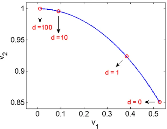
Recall we supposed vw >0. If vw ≯0, let (K, L) be the indexes defined in (3.3). The above result holds for v(K)w(L) >0 with the matrix Md(K, L). For dsufficiently large, v(K)w(L) is then close to a feasible solution of (MBP) for Md(K, L). Adding zero to this feasible solution gives a feasible solution for Mb. Example 1. Let Md= −d 1 1 1 . Clearly, 0 1 0 1
belongs to the set B, i.e. it corresponds to maximal biclique of the graph generated by Mb. By Theorem 6, for d >1, it belongs to Sd i.e. [(0 1)T,(0 1)] is stationary points of (NF-1d).
For d > 1, one can also check that the singular values of Md are disjoint and that the second pair
of singular vectors is positive. Since it is a positive stationary point of the unconstrained problem, it is also a stationary point of (NF-1d). As d goes to infinity, it must get closer to a biclique of
(MBP) (Theorem 7). Moreover Md is symmetric so that the right and left singular vectors are equal
to each other. Figure 2 shows the evolution5 of this positive singular vector of Mdwith respect tod. It
converges to(0 1)and then the product of the left and right singular vector converges to
0 0 0 1 ∈F. Figure 2: Evolution of (v1v2)T(v1v2) ∈ Sd. 5
By Wedin’s theorem (cf. matrix perturbation theory, see e.g. [28]), singular subspaces of Md associated with a positive singular value are continuously deformed with respect tod.
3.3 Multiplicative Updates for Nonnegative Factorization
In this section, the MU of Lee and Seung presented in Section 2.2 to find approximate solutions of (NMF) are generalized to (NF). Other than providing a way of computing approximate solutions of (NF), this result will also help us to understand why the updates of Lee and Seung are not very efficient in practice.
The Karush-Kuhn-Tucker optimality conditions of the (NF) problem are the same as for (NMF) (see Section 2.2). Of course, any real matrix M can be written as the difference of two nonnegative matrices: M =P−N withP, N ≥0. This can be used to generalize the algorithm of Lee and Seung. In fact, (2.5) and (2.6) become
V ◦(V W WT +N WT) = V ◦(P WT) (3.13)
W ◦(VTV W+VTN) = W ◦(VTP) (3.14) and using the same idea as in Section 2.2, we get the following multiplicative update rules :
Theorem 8. For V, W ≥ 0 and M = P −N with P, N ≥ 0, the cost function ||M −V W||F is nonincreasing under the following update rules:
V ←V ◦ [P W
T]
[V W WT +N WT], W ←W ◦
[VTP]
[VTV W +VTN]. (3.15)
Proof. We only treat the proof forV since the problem is perfectly symmetric. The cost function can be split intomindependent components related to each row of the error matrix, each depending on a specific row ofP,N andV, which we call respectivelyp,nandv. Hence, we can treat each row of V separately, and we only have to show that the function
F(v) = 1
2||p−n−vW|| 2
F. is nonincreasing under the following update
v0 ←v0◦
[pWT] [v0W WT +nWT]
, ∀v0>0. (3.16)
F is a quadratic function so that
F(v) =F(v0) + (v−v0)∇F(v0) + 1
2(v−v0)∇ 2F(v
0)(v−v0)T, ∀v0,
with∇F(v0) = (−p+n+v0W)WT and ∇2F(v0) =W WT. LetGbe a quadratic model ofF around
v0: G(v) =F(v0) + (v−v0)∇F(v0) + 1 2(v−v0)K(v0)(v−v0) T withK(v0) = diag [v0W WT+nWT] [v0]
. G has the following nice properties (see below): (1) Gis an upper approximation of F i.e. G(v)≥F(v),∀v;
(2) The global minimum ofG(v) is nonnegative and given by (3.16).
Therefore, the global minimum of G, given by (3.16), provides a new iterate which guarantee the monotonicity ofF. In fact,
F(v0) =G(v0)≥min
v G(v) =G(v ∗
It remains to show that (1) and (2) hold.
(1)G(v)≥F(v)∀v. This is equivalent toK(v0)−W WT positive semidefinite (PSD). Lee and Seung have proved [22] that A= diag
[v0W WT] [v0]
−W WT is PSD (see also [17]). Since B = diag
[nWT] [v0]
is a diagonal nonnegative matrix forv0 >0 andnWT ≥0,A+B =K(v0)−W WT is also PSD. (2) The global minimum ofG is given by (3.16):
v∗ = argminvG(v) = v0−K−1(v0)∇F(v0) = v0−v0◦ [−pWT + (v0W WT +nWT)] [v0W WT +nWT] = v0◦ [pWT] [v0W WT +nWT] .
As with standard multiplicative updates, convergence can be guaranteed with a simple modifica-tion:
Theorem 9. For every constant > 0 and for M = P −N with P, N ≥ 0, ||M −V W||F is nonincreasing under V ←max , V ◦ [P W T] [V W WT +N WT] , W ←max , W ◦ [V TP] [VTV W +VTN] (3.17)
for any (V, W) ≥ . Moreover, every limit point of this algorithm is a stationary point of the opti-mization problem (2.9).
Proof. We use exactly the same notation as in the proof of Theorem 3.15, so that F(v0) =G(v0)≥min
v≥ G(v) =G(v
∗)≥F(v∗), v
0≥
remains valid. By definition,K(v0) is a diagonal matrix implying thatG(v)is the sum ofr independent quadratic terms, each depending on a single entry of v. Therefore,
argminv≥G(v) = max, v0◦
[pWT] [v0W WT +nWT]
, and the monotonicity is proved.
Let ( ¯V ,W¯) be a limit point of a sequence {(Vk, Wk)}generated by (3.17). The monotonicity implies that {||M −VkWk||F} converges to ||M −V¯W¯||F since the cost function is bounded from below. Moreover, ¯ Vik = max , αik V¯ik , ∀i, k (3.18) where αik = Pi: ¯ WkT: ¯ Vi:W¯W¯kT:+Ni:W¯kT: ,
which is well-defined since ¯Vi:W¯W¯kT: >0. One can easily check that the stationarity conditions of (2.9) for ¯V are
¯
Vik≥, αik ≤1 and ( ¯Vik−) (αik−1) = 0, ∀i, k.
Finally, by (3.18), we have either ¯Vik=and αik ≤1, or ¯Vik > and αik = 1,∀i, k. The same can be done for ¯W by symmetry.
In order to implement the updates (3.15), one has to choose the matricesP andN. It is clear that
∀P, N ≥0 such that M =P −N, there exists a matrix C ≥0 such that the two components P and N can be written P = M++C and N = M−+C. When C goes to infinity, the above updates do not change the matrices V and W, which seems to indicate that smaller values of C are preferable. Indeed, in the caser = 1, one can prove thatC=0 is an optimal choice:
Theorem 10. ∀P, N ≥0 s.t. M =P−N, and ∀v∈Rn +, w∈Rm+: ||M−v1w||F ≤ ||M −v2w||F ≤ ||M−vw||F, (3.19) for v1 =v◦ [M+wT] [vwwT +M−wT] and v2 =v◦ [P wT] [vwwT +N wT].
Proof. The second inequality of (3.19) is a consequence of Theorem 3.15. For the first one, we treat the inequality separately for each entry ofv i.e. we prove that
||Mi:−v1iw||F ≤ ||Mi:−v2iw||F, ∀i. Let definevi∗ as the optimal solution of the unconstrained problem i.e.
vi∗= argminvi||Mi:−viw||F =
Mi:wT
wwT ,
and a, b, d≥0,e >0, as
a= (M+)i:wT, b= (M−)i:wT, d= (P−M+)i:wT and e=viwwT.
Noting thatP −M+=N −M−, we have
vi∗=vi a−b e , v1i =vi a e+b and v2i=vi a+d e+b+d . Supposev∗i ≥vi. Therefore, a−b e ≥1 ⇒ a−b−e≥0 ⇒ a−b e ≥ a e+b.
Moreover, 1≤ e+a+b+dd sincev2i is a better solution thanvi (Theorem 3.15). Finally, 1≤ a+d e+b+d ≤ a e+b ≤ a−b e ⇒ vi≤v2i≤v1i≤v ∗ i. The casevi∗≤vi is similar.
Unfortunately, this result does not hold for r >1. This is even true for nonnegative matrices, i.e. one can improve the effect of a standard Lee and Seung multiplicative update by using a well-chosen matrixC.
Example 2. With the following matrices
M = 0 0 1 0 1 1 1 1 0 , V = 1 1 1 0 1 1 , W = 1 0 0 1 0 1 and C= 0 0 1 0 0 0 1 0 0 ,
we have ||M −V0W||F < ||M −V00W||F where V0 (resp. V00) is updated following (3.15) using
P =M +C andN =C (resp. P =M and N =0).
However, in practice, it seems that the choice of a proper matrixC is nontrivial and cannot accelerate significantly the speed of convergence.
4
How good are the Multiplicative Updates (MU) of Lee and Seung?
In this section, we use Theorem 8 to interpret the multiplicative rules for (NMF) and show why the HALS algorithm performs much better in practice.4.1 An Improved Version of the MU
The aim of the MU is to improve a current solution (V, W) ≥ 0 by optimizing alternatively V (W fixed), and vice-versa. In order to prove the monotonicity of the MU,||M−V W||F was shown to be nonincreasing under an update of a single row of V (resp. column of W) since the objective function can be split intom (resp. n) independent quadratic terms, each depending on the entries of a row of V (resp. column of W); cf. proof of Theorem 8.
However, there is no guarantee, a priori, that the algorithm is also nonincreasing with respect to an individual update of a column of V (resp. row of W). In fact, each entry of a column of V (resp. row ofW) depends on the other entries of the same row (resp. column) in the cost function. The next theorem states that this property actually holds.
Corollary 2. ForV, W ≥0, ||M−V W||F is nonincreasing under
V:k←V:k◦
[M WkT:]
[V W WkT:], Wk:←Wk:◦
[V:TkM]
[V:TkV W], ∀k, (4.1)
i.e. under the update of any column of V or any row of W using the MU (2.7). Proof. This is a consequence of Theorem 8 usingP =M and N =P
i6=kV:iWi:. In fact,||M−V W||F =||(M−P
i6=kV:iWi:)−V:kWk:||F.
Corollary 2 sheds light on a very interesting fact: the multiplicative updates are also trying to optimize alternatively the columns of V and the rows of W using a specific cyclic order: first, the columns ofV and then the rows of W. We can now point out two ways of improving the MU:
1. When updating a column ofV (resp. a row of W), the columns (resp. rows) already updated are not taken into account: the algorithm uses their old values;
2. The multiplicative updates are not optimal: P 6=M+andN 6=M−(cf. Theorem 10). Moreover, there is actually a closed-form solution for these subproblems (cf. HALS algorithm, Section 2.3). Therefore, using Theorem 10, we have the following new improved updates
Corollary 3. ForV, W ≥0, ||M−V W||F is nonincreasing under V:k ←V:k◦ [(Rk)+WkT:] [V:kWk:WkT:+ (Rk)−WkT:] , Wk:←Wk:◦ [V:kT(Rk)+] [VT :kV:kWk:+V:Tk(Rk)−] , ∀k, (4.2) with Rk = M− P
i6=kV:iWi:. Moreover, the updates (4.2) perform better than the updates (4.1), but
worse than the updates (2.12-2.13) which are optimal.
Proof. This is a consequence of Theorem 8 and 10 using P = (Rk)+ and N = (Rk)−. In fact,||M−V W||F =||Rk−V:kWk:||F.
4.2 An example
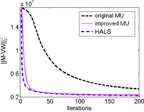
Figure 3 shows an example of the behavior of the different algorithms: the original MU (Section 2.2), the improved version (Corollary 3) and theoptimal HALS method (Section 2.3). The test was carried out on a commonly used data set for NMF: the cbcl face database6; 2429 faces (columns) consisting each of 19×19 pixels (rows) for which we set r = 40 and we used the same scaled (see Remark 3 below) random initialization and the same cyclic order (same as the MU i.e. first the columns of V then the rows of W) for the three algorithms. We observe that the MU converges significantly less
Figure 3: Comparison of the MU of Lee and Seung (2.7), the optimal rank-one NF multiplicative updates (4.2) and the HALS (2.12-2.13) applied to the cbcl face database.
rapidly than the two other algorithms. There do not seem to be good reasons to use either the MU or the method of Corollary 3 since there is a closed-form solution (2.12-2.13) for the corresponding subproblems.
Finally, the HALS algorithm has the same computational complexity [16] and performs provably much better than the popular multiplicative updates of Lee and Seung. Of course, because of the NP-hardness of (NMF) and the existence of numerous locally optimal solutions, it is not possible to give a theoretical guarantee that HALS will converge to a better solution than the MU: although its iterations arelocally more efficient, they could still end up at a worse local optimum.
Remark 2. For r = 1, one can check that the three algorithms above are equivalent for (NMF). Moreover, they correspond to the power method [13] which converges to the optimal rank-one solution, given that it is initialized with a vector which is not perpendicular to the singular vector corresponding to the maximum singular value.
Remark 3. We say that (V, W) is scaled if the optimal solution to the problem
min
α∈R||M −αV W||F (4.3)
is equal to 1. Obviously, any stationary point is scaled ; the next Theorem is an extension of a result of Ho et al. [18].
6
CBCL Face Database #1, MIT Center For Biological and Computation Learning. Available athttp://cbcl.mit.edu/cbcl/sof tware-datasets/F aceData2.html.
Theorem 11. The following statements are equivalent (1) (V, W) is scaled; (2) V W is on the boundary of BM 2, 1 2||M||F
, the ball centered at M2 of radius 12||M||F; (3) ||M−V W||2
F =||M||2F − ||V W||2F (and then ||M||2F ≥ ||V W||2F).
Proof. The solution of (4.3) can be written in the following closed form
α= hM, V Wi
hV W, V Wi, (4.4)
wherehA, Bi=P
ijAijBij =trace(ABT) is the scalar product associated with the Frobenius norm.
Sinceα = 1, hV W −M, V Wi = 0 hV W −M, V Wi+ M 2 , M 2 = M 2 , M 2 M 2 −V W, M 2 −V W = M 2 , M 2 , so that (1) and (2) are equivalent. For the equivalence of (1) and (3), we have
hM−V W, M −V Wi = ||M||F2 −2hM, V Wi+||V W||2F
= ||M||2F − ||V W||F2 −2hM, V Wi − hV W, V Wi.
= ||M||2F − ||V W||2F
if and only ifhM, V Wi=hV W, V Wi.
Theorem 11 can be used as follows: when you compute the error of the current solution, you can scale it without further computational cost. In fact,
||M−V W||2F = hM−V W, M−V Wi
= ||M||2F −2hM, V Wi+||V W||2F. (4.5)
Note that the third term of (4.5) can be computed inO(max(m, n)r2) operations since
||V W||2F = X ij X k Vik2Wkj2 + 2X ij X k6=l VikWkjVilWlj = X k X i Vik2 X j Wkj2+ 2X k6=l X i VikVil X j WkjWlj = ||(VTV)◦(W WT)||1 where||A||1=P
ij|Aij|. This is especially interesting for sparse matrices since only a small number of the entries ofV W (which could be dense) need to be computed to evaluate the second term of (4.5).
5
Biclique Finding Algorithm
In this section, an algorithm for the maximum edge biclique problem whose main iteration requires O(|E|) operations is presented. It is based on the multiplicative updates for Nonnegative Factorization and the strong relation between these two problems (Theorems 4, 6 and 7). We compare the results with other algorithms with iterates requiring O(|E|) operations using the DIMACS database and random graphs.
5.1 Description
For d sufficiently large, stationary points of (NF-1d) are close to bicliques of (MBP) (Theorem 7). Moreover, the two problems have the same cost function. One could then think of applying an algorithm that finds stationary points of (NF-1d) in order to localize a large biclique of the graph generated byMb. This is the idea of Algorithm 1 using the multiplicative updates (3.15) with
P = (Md)+=Mb and N = (Md)− =d(1m×n−Mb).
A priori, it is not clear what valuedshould take. Following the spirit of homotopy methods, we chose to start the algorithm with a small value ofdand then to increase it until the algorithm converges to a biclique of (MBP).
Algorithm 1 Biclique Finding Algorithm inO(|E|) operations
Require: Mb∈ {0,1}m×n,v∈Rm++,w∈Rn++,d=d0>0,α >1. 1: fork= 1,2, . . . do 2: v ← v ◦ [Mbw T] [v||w||2 2+d(1m||w||1−MbwT)] (5.1) w ← w◦ [v TM b] [||v||2 2w+d(1n||v||1−vTMb)] (5.2) d = αd 3: end for
We observed that initial value ofdshould not be chosen too large: otherwise, the algorithm often converges to the trivial solution: the empty biclique. In fact, in that case, the denominators in (5.1) and (5.2) will be large, even during the initial steps of the algorithm, and the solution is then forced to converge to zero. Moreover, since the denominators in (5.1) and (5.2) depend on the graph density, the denser the graph is, the greater d0 can be chosen and vice versa. On the other hand, since our algorithm is equivalent to the power method ford= 0 (cf. Remark 2), ifd0 is chosen too small, it will converge to the same solution: the one initialized with the best rank-one approximation ofMb.
For the stopping criterion, one could, for example, wait until the rounding of vw coincides with a feasible solution of (MBP).
5.2 Other Algorithms in O(|E|) operations
We briefly present here two other algorithms to find maximal bicliques using O(|E|) operations per iteration.
5.2.1 Motzkin-Strauss Formalism
In [12], the generalized Motzkin-Strauss formalism for cliques is extended to bicliques by defining the optimization problem max x∈Fα x,y∈F β y xTMby whereFxα={x∈Rn+| Pn i=1xαi = 1},F β y ={y∈Rn+| Pn i=1y β i = 1}and α, β 1.
Nonincreasing multiplicative updates for this problem are then provided:
x←x◦ Mby xTM by 1α , y←y◦ M T b x xTM by β1
This algorithm does not necessarily converge to a biclique: if α and β are not sufficiently small, it may converge to a dense bipartite subgraph (a bicluster). In fact, for α= β = 2, it converges to an optimal rank-one solution of the unconstrained problem as our algorithm does ford= 0. In [12], it is suggested to useα and β around 1.05. Finally, α6=β will favor one side of the biclique. We will use
α=β.
5.2.2 Greedy Heuristic
The simplest heuristic one can imagine is to add, at each step, a vertex which is connected to most vertices in the other side of the bipartite graph. Each time a vertex is selected, the next choices are restricted in order to get a biclique eventually: the vertices which are not connected to the one you have just chosen are deleted. The procedure is repeated on the remaining graph until you get a biclique. One can check that this produces a maximal biclique.
5.3 Results
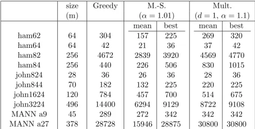
We first present some results for graphs from the DIMACS graph dataset7. We extracted bicliques in those (not bipartite) graphs using the preceding algorithms. We performed 100 runs, 200 iterations each, for the two algorithms with the same initializations. We tried to choose appropriate parame-ters8 for both algorithms. Table 1 displays the cardinality of the biclique extracted by the different algorithms.
Table 2 shows the results for random graphs: we have generated randomly 100 graphs with 100 vertices for different densities (the probability of an edge to belong to the graph is equal to the density). The average numbers of edges in the solutions for the different algorithms are displayed for each density. We kept the same configuration as for the DIMACS graphs (same initializations, 100 runs for each graph, 200 iterations). It seems that the multiplicative updates generates, in general, better solutions, especially when dealing with dense graphs. The algorithm based on the Motzkin-Strauss formalism seems less efficient and is more sensitive to the choice of its parameters.
size Greedy M.-S. Mult.
(m) (α= 1.01) (d= 1,α= 1.1) ham62 ham64 ham82 ham84 john824 john844 john1624 john3224 MANN a9 MANN a27 64 64 256 256 28 70 120 496 45 378 304 42 4672 440 36 182 784 14400 289 28728 mean best 157 225 21 36 2839 3920 226 506 26 36 132 225 457 700 6294 9129 272 342 15946 28875 mean best 269 320 37 42 4569 4770 830 1015 28 36 220 225 514 675 8722 9108 342 342 30800 30800 Table 1: Solutions for DIMACS data: number of edges in the bicliques.
7
f tp://dimacs.rutgers.edu/pub/challenge/graph/benchmarks/clique.
8
For the M.-S. algorithm: the alternative choices of parametersα= 1.005 andα= 1.05 for the DIMACS graphs and
α= 1.005 andα= 1.1 for the random graphs were tested and all gave worse results. Small changes to the parameters of the Mult. algorithm led to similar results, so that it seems less sensitive to the choice of its parameters than the M.-S. algorithm.
density Greedy M.-S. M.-S. Mult. (α= 1.01) (α= 1.05) (d= 1,α= 1.1) 0.1 0.2 0.3 0.4 0.5 0.6 0.7 0.8 0.9 8.9 15.8 24.2 37.7 58.8 92.5 158.4 311.0 806.8 mean best 10.4 18.9 14.5 29.8 18.9 38.7 24.0 51.2 31.7 69.0 43.4 93.7 63.6 133.4 106.0 207.1 241.9 431.3 mean best 14.4 19.2 23.7 31.5 33.8 43.4 46.9 61.3 65.8 86.7 90.5 127.9 117.9 190.0 154.4 261.5 88.1 235.4 mean best 14.4 19.2 23.9 31.5 34.1 43.3 47.0 61.0 67.6 87.0 101.7 127.8 172.2 202.4 328.0 342.3 828.1 828.1 Table 2: Solutions for random graphs: average number of edges in the bicliques.
Remark 4. Algorithm 1 enjoys some flexibility:
• It is applicable to non-binary matrices i.e. weighted graphs.
• It is possible to favor one side of the biclique. In fact, the multiplicative updates for NF can be adapted using the same developments as in Section 3.3 to cost functions with regularization terms, e.g.
min
v,w≥0 ||M−vw||
2
F +α||v||22+β||w||22.
• If d is kept sufficiently small, for example replacing d = αd by d = min(αd, dm) for some
dm > 0, there is no guarantee that the algorithm will converge to a biclique. However, the
negative entries in Md will enforce the corresponding entries of the solutions of (NF-1d) to
be small (recall that Theorem 7 states that, for d sufficiently large, they will be equal to zero). Therefore, by rounding these solutions, instead of a biclique, one gets a dense submatrix of Mb
i.e. a bicluster. Algorithm 1 can then be used as a biclustering algorithm. The density of the corresponding submatrix will depend on the choice of dm. Table 3 gives an example of such behavior.
dm 0.01 0.05 0.1 0.5 1 1.5
size 5412 4428 2952 1073 595 539 density 29% 31% 35% 42% 51% 52%
Table 3: Biclusters for the ’classic’ text mining dataset (7094 texts and 41681 words with more than 99.9% of entries equal to zero) with parametersd0= 10−5, α= 1.025,maxiter = 500.
6
Conclusion
We have introduced Nonnegative Factorization (NF), a new variant of Nonnegative Matrix Factoriza-tion (NMF), and proved its NP-hardness for any fixed rank by reducFactoriza-tion to the maximum edge biclique problem. The multiplicative updates for NMF can be generalized to NF and provide a new interpre-tation of the algorithm of Lee and Seung, which explains why it does not perform well in practice. We also developed an heuristic algorithm for the biclique problem whose iterations require O(|E|) operations, based on theoretical results about stationary points of a specific rank-one nonnegative factorization problem (NF-1d) and the use of multiplicative updates.
To conclude, we point out that none of the algorithms presented in this paper is guaranteed to converge to a globally optimal solution (and, to the best of our knowledge, such an algorithm has not been proposed yet) ; this is in all likelihood due to the NP-hardness of the NMF and NF problems. Indeed, only convergence to a stationary point has been proved for the algorithms of Sections 2 and 3, a property which, while desirable, provides no guarantee about the quality of the solution obtained (for example, nothing prevents these methods from converging to a stationary but rank-deficient solution, which in most cases could be further improved). Finally, no convergence proof for the biclique finding algorithm introduced in Section 5 is provided (convergence results from the preceding sections no longer hold because of the dynamic updates of parameter d) ; however, this heuristic seems to give very satisfactory results in practice.
References
[1] A. Berman and R. Plemmons,Rank factorization of nonnegative matrices, SIAM Review, 15
(3) (1973), p. 655.
[2] M. Berry, M. Browne, A. Langville, P. Pauca, and R. Plemmons, Algorithms and
Applications for Approximate Nonnegative Matrix Factorization, Computational Statistics and Data Analysis, 52 (2007), pp. 155–173.
[3] D. P. Bertsekas, Nonlinear Programming: Second Edition, Athena Scientific, Massachusetts, 1999.
[4] M. Biggs, A. Ghodsi, and S. Vavasis,Nonnegative Matrix Factorization via Rank-One Down-date. Preprint, June 2007.
[5] D. Chen and R. Plemmons,Nonnegativity Constraints in Numerical Analysis. Paper presented at the Symposium on the Birth of Numerical Analysis, Leuven Belgium. To appear in the Con-ference Proceedings, to be published by World Scientific Press, A. Bultheel and R. Cools, Eds., 2007.
[6] C. Cichocki, R. Zdunek, and S. Amari,Hierarchical ALS Algorithms for Nonnegative Matrix and 3D Tensor Factorization, in ICA07, London, UK, September 9-12, Lecture Notes in Computer Science, Vol. 4666, Springer, pp. 169-176, 2007.
[7] ,Nonnegative Matrix and Tensor Factorization, IEEE Signal Processing Magazine, (2008), pp. 142–145.
[8] J. Cohen and U. Rothblum, Nonnegative ranks, Decompositions and Factorization of
Non-negative Matrices, Linear Algebra and its Applications, 190 (1993), pp. 149–168.
[9] K. Devarajan,Nonnegative Matrix Factorization: An Analytical and Interpretive Tool in Com-putational Biology, PLoS Computational Biology, 4(7), e1000029 (2008).
[10] I. Dhillon, D. Kim, and S. Sra,Fast Newton-type Methods for the Least Squares Nonnegative Matrix Approximation Problem, in Proceedings of SIAM Conf. on Data Mining, 2007.
[11] I. Dhillon and S. Sra, Nonnegative Matrix Approximations: Algorithms and Applications,
tech. report, University of Texas (Austin), 2006. Dept. of Computer Sciences.
[12] C. Ding, Y. Zhang, T. Li, and S. Holbrook, Biclustering Protein Complex Interactions
with a Biclique Finding Algorithm, in Sixth IEEE International Conference on Data Mining, 2006, pp. 178–187.
[13] N. Gillis, Approximation et sous-approximation de matrices par factorisation positive: algo-rithmes, complexit´e et applications, master’s thesis, Universit´e catholique de Louvain, 2007. In French.
[14] N. Gillis and F. Glineur,Nonnegative Matrix Factorization and Underapproximation. Com-munication at 9th International Symposium on Iterative Methods in Scientific Computing, Lille, France, 2008.
[15] G. Golub and C. Van Loan,Matrix Computation, 3rd Edition, The Johns Hopkins University Press Baltimore, 1996.
[16] N.-D. Ho,Nonnegative Matrix Factorization - Algorithms and Applications, PhD thesis, Univer-sit´e catholique de Louvain, 2008.
[17] N.-D. Ho, P. Van Dooren, and V. Blondel, Weighted Nonnegative Matrix Factorization
and Face Feature Extraction. Submitted to Image and Vision Computing, 2007. [18] ,Descent Type Algorithms for NMF. arXiv:0801.3199v2, 2008.
[19] P. Hoyer,Nonnegative Matrix Factorization with Sparseness Constraints, J. Machine Learning Research, 5 (2004), pp. 1457–1469.
[20] H. Kim and H. Park,Non-negative Matrix Factorization Based on Alternating Non-negativity Constrained Least Squares and Active Set Method, SIAM J. Matrix Anal. Appl., 30(2) (2008), pp. 713–730.
[21] D. Lee and H. Seung, Learning the Parts of Objects by Nonnegative Matrix Factorization, Nature, 401 (1999), pp. 788–791.
[22] ,Algorithms for Non-negative Matrix Factorization, In Advances in Neural Information Pro-cessing, 13 (2001).
[23] C.-J. Lin,On the Convergence of Multiplicative Update Algorithms for Nonnegative Matrix Fac-torization, in IEEE Transactions on Neural Networks, 2007.
[24] , Projected Gradient Methods for Nonnegative Matrix Factorization, Neural Computation, 19 (2007), pp. 2756–2779. MIT press.
[25] P. Paatero and U. Tapper, Positive matrix factorization: a non-negative factor model with optimal utilization of error estimates of data values, Environmetrics, 5 (1994), pp. 111–126. [26] R. Peeters,The maximum edge biclique problem is NP-complete, Discrete Applied Mathematics,
131(3) (2003), pp. 651–654.
[27] M. Powell,On Search Directions for Minimization Algorithms, Mathematical Programming, 4 (1973), pp. 193–201.
[28] G. Stewart and J.-g. Sun,Matrix Perturbation Theory, Academic Press, San Diego, 1990. [29] L. Thomas, Rank factorization of nonnegative matrices, SIAM Review, 16(3) (1974), pp. 393–
394.
Recent titles
CORE Discussion Papers
2008/26. Leonidas C. KOUTSOUGERAS and Nicholas ZIROS. Decentralization of the core through Nash equilibrium.
2008/27. Jean J. GABSZEWICZ, Didier LAUSSEL and Ornella TAROLA. To acquire, or to compete?
An entry dilemma.
2008/28. Jean-Sébastien TRANCREZ, Philippe CHEVALIER and Pierre SEMAL. Probability masses fitting in the analysis of manufacturing flow lines.
2008/29. Marie-Louise LEROUX. Endogenous differential mortality, non monitored effort and optimal non linear taxation.
2008/30. Santanu S. DEY and Laurence A. WOLSEY. Two row mixed integer cuts via lifting.
2008/31. Helmuth CREMER, Philippe DE DONDER, Dario MALDONADO and Pierre PESTIEAU.
Taxing sin goods and subsidizing health care.
2008/32. Jean J. GABSZEWICZ, Didier LAUSSEL and Nathalie SONNAC. The TV news scheduling game when the newscaster's face matters.
2008/33. Didier LAUSSEL and Joana RESENDE. Does the absence of competition in the market foster competition for the market? A dynamic approach to aftermarkets.
2008/34. Vincent D. BLONDEL and Yurii NESTEROV. Polynomial-time computation of the joint spectral radius for some sets of nonnegative matrices.
2008/35. David DE LA CROIX and Clara DELAVALLADE. Democracy, rule of law, corruption incentives and growth.
2008/36. Jean J. GABSZEWICZ and Joana RESENDE. Uncertain quality, product variety and price competition. 2008/37. Gregor ZOETTL. On investment decisions in liberalized electricity markets: the impact of price caps at the spot market.
2008/38. Helmuth CREMER, Philippe DE DONDER, Dario MALDONADO and Pierre PESTIEAU.
Habit formation and labor supply.
2008/39. Marie-Louise LEROUX and Grégory PONTHIERE. Optimal tax policy and expected
longevity: a mean and variance approach.
2008/40. Kristian BEHRENS and Pierre M. PICARD. Transportation, freight rates, and economic geography.
2008/41. Gregor ZOETTL. Investment decisions in liberalized electricity markets: A framework of peak load pricing with strategic firms.
2008/42. Raouf BOUCEKKINE, Rodolphe DESBORDES and Hélène LATZER. How do epidemics
induce behavioral changes?
2008/43. David DE LA CROIX and Marie VANDER DONCKT. Would empowering women initiate the
demographic transition in least-developed countries?
2008/44. Geoffrey CARUSO, Dominique PEETERS, Jean CAVAILHES and Mark ROUNSEVELL.
Space-time patterns of urban sprawl, a 1D cellular automata and microeconomic approach.
2008/45. Taoufik BOUEZMARNI, Jeroen V.K. ROMBOUTS and Abderrahim TAAMOUTI. Asymptotic
properties of the Bernstein density copula for dependent data.
2008/46. Joe THARAKAN and Jean-Philippe TROPEANO. On the impact of labor market matching on
regional disparities.
2008/47. Shin-Huei WANG and Cheng HSIAO. An easy test for two stationary long processes being uncorrelated via AR approximations.
2008/48. David DE LA CROIX. Adult longevity and economic take-off: from Malthus to Ben-Porath.
2008/49. David DE LA CROIX and Gregory PONTHIERE. On the Golden Rule of capital accumulation
under endogenous longevity.
2008/50. Jean J. GABSZEWICZ and Skerdilajda ZANAJ. Successive oligopolies and decreasing returns.
2008/51. Marie-Louise LEROUX, Pierre PESTIEAU and Grégory PONTHIERE. Optimal linear taxation
under endogenous longevity.
2008/52. Yuri YATSENKO, Raouf BOUCEKKINE and Natali HRITONENKO. Estimating the dynamics
Recent titles
CORE Discussion Papers - continued
2008/53. Roland Iwan LUTTENS and Marie-Anne VALFORT. Voting for redistribution under desert-sensitive altruism.
2008/54. Sergei PEKARSKI. Budget deficits and inflation feedback.
2008/55. Raouf BOUCEKKINE, Jacek B. KRAWCZYK and Thomas VALLEE. Towards an
understanding of tradeoffs between regional wealth, tightness of a common environmental constraint and the sharing rules.
2008/56. Santanu S. DEY. A note on the split rank of intersection cuts.
2008/57. Yu. NESTEROV. Primal-dual interior-point methods with asymmetric barriers.
2008/58. Marie-Louise LEROUX, Pierre PESTIEAU and Gregory PONTHIERE. Should we subsidize longevity?
2008/59. J. Roderick McCRORIE. The role of Skorokhod space in the development of the econometric analysis of time series.
2008/60. Yu. NESTEROV. Barrier subgradient method.
2008/61. Thierry BRECHET, Johan EYCKMANS, François GERARD, Philippe MARBAIX, Henry
TULKENS and Jean-Pascal VAN YPERSELE. The impact of the unilateral EU commitment on the stability of international climate agreements.
2008/62. Giorgia OGGIONI and Yves SMEERS. Average power contracts can mitigate carbon leakage. 2008/63. Jean-Sébastien TANCREZ, Philippe CHEVALIER and Pierre SEMAL. A tight bound on the
throughput of queueing networks with blocking.
2008/64. Nicolas GILLIS and François GLINEUR. Nonnegative factorization and the maximum edge biclique problem.
Books
Y. POCHET and L. WOLSEY (eds.) (2006), Production planning by mixed integer programming. New York, Springer-Verlag.
P. PESTIEAU (ed.) (2006), The welfare state in the European Union: economic and social perspectives. Oxford, Oxford University Press.
H. TULKENS (ed.) (2006), Public goods, environmental externalities and fiscal competition. New York, Springer-Verlag.
V. GINSBURGH and D. THROSBY (eds.) (2006), Handbook of the economics of art and culture. Amsterdam, Elsevier.
J. GABSZEWICZ (ed.) (2006), La différenciation des produits. Paris, La découverte.
L. BAUWENS, W. POHLMEIER and D. VEREDAS (eds.) (2008), High frequency financial econometrics: recent developments. Heidelberg, Physica-Verlag.
P. VAN HENTENRYCKE and L. WOLSEY (eds.) (2007), Integration of AI and OR techniques in constraint programming for combinatorial optimization problems. Berlin, Springer.
CORE Lecture Series
C. GOURIÉROUX and A. MONFORT (1995), Simulation Based Econometric Methods. A. RUBINSTEIN (1996), Lectures on Modeling Bounded Rationality.
J. RENEGAR (1999), A Mathematical View of Interior-Point Methods in Convex Optimization.
B.D. BERNHEIM and M.D. WHINSTON (1999), Anticompetitive Exclusion and Foreclosure Through Vertical Agreements.
D. BIENSTOCK (2001), Potential function methods for approximately solving linear programming problems: theory and practice.
R. AMIR (2002), Supermodularity and complementarity in economics. R. WEISMANTEL (2006), Lectures on mixed nonlinear programming.