On the Automatic Construction of
Indistinguishable Operations
M. Barbosa1? and D. Page2
1
Departamento de Inform´atica, Universidade do Minho, Campus de Gualtar, 4710-057 Braga, Portugal.
Department of Computer Science, University of Bristol, Merchant Venturers Building, Woodland Road,
Bristol, BS8 1UB, United Kingdom. [email protected]
Abstract. An increasingly important design constraint for software run-ning on ubiquitous computing devices is security, particularly against physical methods such as side-channel attack. One well studied method-ology for defending against such attacks is the concept of indistinguish-able functions which leak no information about program control flow since all execution paths are computationally identical. However, the constructing such functions by hand is laborious and error prone as their complexity increases. We investigate techniques for automating this pro-cess and find that effective solutions can be constructed with only minor amounts of computational effort.
Keywords.Side-channel Cryptanalysis, Simple Power Analysis, Coun-termeasures, Indistinguishable Operations.
1
Introduction
As computing devices become increasingly ubiquitous, the task of writing soft-ware for them has presented programmers with a number of problems. Firstly, devices like smart-cards are highly constrained in both their computational and storage capacity; due to their low unit cost and small size, such devices are sig-nificantly less powerful than PDA or desktop class computers. This demands selection and implementation of algorithms which are sensitive to the demands of the platform. Coupled with these issues of efficiency, which are also prevalent in normal software development, constrained devices present new problems for the programmer. For example, one typically needs to consider the power charac-teristics and communication frequency of any operation since both eat into the valuable battery life of the device.
Perhaps the most challenging aspect of writing software for ubiquitous com-puters is the issue of security. Performing computation in a hostile, adversarial
?Funded by scholarship SFRH/BPD/20528/2004, awarded by the Funda¸c˜ao para a
environment demands that software is robust enough to repel attackers who hope to retrieve data stored on the device. Although cryptography provides a number of tools to aid in protecting the data, the advent of physical attacks such as side-channel analysis and fault injection mean one needs to consider security of the software implementation as well as the mathematics it implements. By passive monitoring of execution features such as timing variations [14], power consumption [15] or electromagnetic emission [1, 2] attackers can remotely re-cover secret information from a device with little fear of detection. Typically attacks consist of a collection phase which provides the attacker with profiles of execution, and an analysis phase which recovers the secret information from the profiles. Considering power consumption as the collection medium from here on, attack methods can be split into two main classes. Simple power analysis (SPA) is where the attacker is given only one profile and is required to recover the secret information by focusing mainly on the operation being executed. In contrast, differential power analysis (DPA) uses statistical methods to form a corelation between a number of profiles and the secret information by focusing mainly on the data items being processed.
As attack methods have become better understood, so have the related de-fense methods. Although new vulnerabilities are regularly uncovered, one can now deploy techniques in hardware and software which will vastly reduce the effectiveness of most side-channel attacks and do so with fairly minor overhead. Very roughly, defense methods fall into one of two main categories:
Randomisation One method of reducing the chance of leaking secret informa-tion is to introduce a confusion or randomisainforma-tion element into the algorithm being executed. This is particularly effective in defending against DPA-style attacks but may also be useful in the SPA-style case. Essentially, randomisa-tion ensures the execurandomisa-tion sequence and intermediate results are different for every invocation and hence reduces the correlation of a given profile with the secret information. This method exists in many different forms, for example the addition of blinding factors to exponents; dynamically randomising the parameters or control flow in exponentiation algorithms; and using redun-dant representations.
Indistinguishability To prevent leakage of secret information to an SPA-style attack by revealing the algorithm control flow, this approach aims to modify operations sequences so that every execution path is uniform. Again, there are several ways in which this can be achieved. One way is to work directly on the mathematical formulae that define the operations and modify them so that the resulting implementations have identical structure. Another method is to work directly on the code, rearranging it and inserting dummy opera-tions, to obtain the same effect.
Algorithm 1The double-and-add method for ECC point multiplication.
Input: pointP, integerd Output: pointQ=d·P
1: Q← O
2: fori=|d| −1downto0do 3: Q←2·Q
4: if di= 1then
5: Q←Q+P 6: end if 7: end for 8: returnQ
functions to foil SPA style attack is well understood; the general barrier to implementation is how labour intensive and error prone the process is. This is especially true when operation sequences in the functions are more complex than in the stock example of elliptic curve cryptography (ECC), for example systems like XTR or hyperelliptic curve cryptography (HECC). However, the task is ideally suited to automation; to this end our focus in this paper is the realisation of such automation to assist the development of secure software. In the rest of this Section we introduce the concept and use of indistinguishable functions in more detail and present an overview of related work. Then, in Section 2 we describe the construction of such functions as an optimisation problem and offer an algorithm to produce solutions in Section 3. Finally, we present some example results in Section 4 and concluding remarks in Section 5.
1.1 Using Indistinguishable Functions
One of the most basic forms of side-channel attack is that of simple power analysis (SPA): the attacker is presented with a single profile from the collec-tion phase and tasked with recovering the secret informacollec-tion. Such an attack can succeed if one can reconstruct the program control flow by observing the operations performed in an algorithm. If decisions in the control flow are based on secret information, it is leaked to the attacker. Because it represents an ideal partner for constrained devices, we focus here on point multiplication as used in ECC [3] and described by Algorithm 1.
Restricting ourselves to working over the field K = Fp, where p is a large
prime, our elliptic curve is defined by:
E(K) :y2
=x3
+Ax+B
for some parametersAandB. The set of rational pointsP = (x, y) on this curve,
together with the identity elementO, form an additive group. ECC based public
key cryptography typically derives security by presenting an intractable discrete logarithm problem over this curve group. That is, one constructs a secret integer
this operation is hard, one can then transmitQ without revealing the value of
d.
Since one is composed from a different sequence of field operations than the other, point addition and doubling operations will be distinguishable from each
other in a profile of power consumption. Denoting addition byA and doubling
byD, the collection phase presents the attacker with a profile detailing the
oper-ations performed during execution of the algorithm. For example, by monitoring
execution of using the multiplierd= 10012= 910, one obtains the profile:
DADDDA
Given this single profile, the analysis phase can recover the secret value of d
simply by spotting where the point additions occur: if an addition occurs then
di= 1, otherwisedi= 0.
One way to avoid this problem is to employ a double-and-add-always method, due to Coron [7], whereby a dummy addition is executed if the real one is not.
Although the cases where di = 0 and di = 1 are now indistinguishable, this
method significantly reduces the performance of the algorithm since many more additions are performed.
However, the ECC group law is very flexible in terms of how the point ad-dition and doubling operations can be implemented through different curve pa-rameterisations, point representations and so on. We can utilise this flexibility to consider forcing indistinguishability by manipulating the functions for point addition and doubling so that they are no longer different. This is generally achieved by splitting the more expensive point addition into two parts, each of which is identical in terms of the operations it performs to a point doubling. Put more simply, instead of recovering the profile above from the SPA collection phase, an attacker gets:
DDDDDDDD
from which they can get no useful information. Note that although we present the use of indistinguishable functions solely for point multiplication or exponen-tiation, the technique is more generally useful and can be applied in many other contexts.
1.2 Related Work
Gebotys and Gebotys [11] analyse the SPA resistance of a DSP-based implemen-tation of ECC point multiplication using projective coordinates on curves over
Fp. They show that by hand-modifying the doubling and adding implementation
code, simply by inserting dummy operations, it is possible to obtain significant improvements. Likewise, Trichina and Bellezza [20] analyse the overhead
associ-ated with the same approach using mixed coordinates on curves overF2n, and
and Smart [17] take a different approach by finding different curve parameter-isations that offer naturally indistinguishable formula; they utilise Hessian and Jacobi form elliptic curves respectively.
In other contexts than ECC, Page and Stam [19] present hand-constructed indistinguishable operations for XTR.
Chevallier-Mames et al. [6] propose a generalised formulation for construct-ing indistconstruct-inguishable functions and apply it to processor-level sequences of in-structions. SPA attacks typically exploit conditional instructions that depend on secret information: the solution is to make the sequences of instructions (pro-cesses) associated with both branches indistinguishable. The authors introduce the concept of side channel atomicity: all processes are transformed, simply by padding them with dummy operations, so that they execute as a repetition of a small instruction sequence (a pattern) called a side-channel atomic block.
2
Indistinguishable Functions
In this section we enunciate the problem of building indistinguishable functions as an optimisation problem. We begin by defining a problem instance.
Definition 1. Let F be a list of N functions F = F1, F2, ..., FN where each
function Fi is itself a list of instructions from a finite basic instruction setL:
Fi=Fi[1], Fi[2], ..., Fi[|Fi|]
where |Fi| denotes the length of functionFi, and Fi[j] ∈L denotes instruction
j of function Fi, with 1 ≤j ≤ |Fi|. Also, let Fi[k..j] denote instructions k toj
in functionFi, with1≤k≤j≤ |Fi|.
For concreteness one should think of the simple case of two functionsF1andF2
as performing ECC point addition and doubling. Further, the instruction setL
is formed from three-address style operations [18] on elements in the base field, for example addition and multiplication, and the functions are straight-line in that they contain no internal control flow structure.
We aim to manipulate the original functions into new versionsF0
i such that
the execution trace of all of them is some multiple of the execution trace of
some patternΠ. Clearly we might need to add some dummy instructions to the
original functions as well as reordering their instructions so that the pattern is followed. To allow for instruction reordering, we extend our problem definition to include information about the data dependencies between instructions within each function. We represent these dependencies as directed graphs.
Definition 2. Given a set F as in Definition 1, let P be the list of pairs
P = (F1, G1),(F2, G2), ...,(FN, GN)
where Gi = (Vi, Ei) is a directed graph in which Vi and Ei are the associated
Fi[j], associate node vj ∈ Vi. Let Ei contain an edge between nodes vj and vk
if and only if executing instruction Fi[j] before instruction Fi[k] disrupts the
normal data flow inside the function. We say that instruction Fi[j] depends on
instructionFi[k].
In general terms, given a straight-line functionFi described using three-address
operations from our instruction set L, the pair of function and graph (Fi,Gi)
can be constructed as follows:
1. Add|Fi| nodes toVi so that each instruction in the function is represented
by a node in the graph.
2. For every instructionFi[j] add an edge (vj, vk) toEiif and only ifFi[j] uses
a result directly modified by some instruction Fi[k]. Note that we assume
that symbols for intermediate results are not reused; that is the function is in single-static-assignment (SSA) form [18]. If reuse is permitted, additional edges must be inserted in the dependency graph to prevent overwriting in-termediate results.
3. Calculate (Vi, Ei0), the transitive closure of the graph (Vi, Ei), and takeGi=
(Vi, Ei0).
We use the dependency graphs in Definition 2 to guarantee that the
transforma-tions we perform on the functransforma-tionsFiare sound. That is, as long as we respect the
dependencies, the program is functionally correct even though the instructions are reordered. Definition 3 captures this notion.
Definition 3. A functionFi0 is a valid transformation of a functionFi (written
Fi0WFi) if given the dependency graphGi,Fi0 can be generated by modifyingFi
as follows:
1. Reorder the instructions in Fi, respecting the dependency graph Gi i.e. if
there is an edge(vj, vk)∈Ei then instructionFi[j]must occur after
instruc-tionFi[k] inFi0.
2. Insert a finite number of dummy instructions.
The goal is to find Π and matching F0
i whose processing overhead compared
to the original programs is minimised. Hence, our problem definition must also include the concept of computational cost. For the sake of generality, we assign
to each basic instruction in setLan integer weight value that provides a relative
measure of it’s computational weight.
Definition 4. Let ω :L→Nbe a weight function that, for each basic
instruc-tion l ∈L, provides a relative value ω(l) for the computational load associated
with instruction l.
For example, takingw(x+y) = 1 we could setw(x2
Algorithm 2Methods for ECC affine point addition (left) and doubling (right).
Input: P = (x1, y1), Q= (x2, y2) Output: R= (x3, y3) =P+Q
1: λ1←y2−y1 2: λ2←x2−x1 3: λ3←λ−
1 2 4: λ4←λ1·λ3 5: λ5←λ
2 4 6: λ6←λ5−x1 7: x3←λ6−x2 8: λ7←x1−x3 9: λ8←λ4·λ7 10: y3←λ8−y1
Input: P = (x1, y1)
Output: R= (x3, y3) = 2·P 1: λ1←x
2 1 2: λ2←λ1+λ1 3: λ3←λ2+λ1 4: λ4←λ3+A 5: λ5←y1+y1 6: λ6←λ−
1 5 7: λ7←λ4·λ6 8: λ8←λ
2 7 9: λ9←x1+x1 10: x3←λ8−λ9 11: λ10←x1−x3 12: λ11←λ10·λ7 13: y3 ←λ11−y1
Definition 5. Given a pair (P, ω) as in Definitions 1, 2 and 4, find a pattern
Π and a list of functionsF0=F1, F0 2, ..., F0 0
N such that
Π =Π[1], Π[2], ..., Π[|Π|] Π[k]∈L,1≤k≤ |Π|
F0
i WFi 1≤i≤N
|F0
i|= 0 (mod|Π|) 1≤i≤N
Fi0[j] =Π[mod(j,|Π|) + 1] 1≤i≤N,1≤j≤ |Fi0| and that
N X
i=1
|F0 i|
X
j=1
ω(Fi0[j])
is minimal.
Intuition on the hardness of satisfying these constraints comes from noticing similarities with well-known NP-complete optimisation problems such as the Minimum Bin Packing, Longest Common Subsequence and Nearest Codeword problems [8].
2.1 A Small Example
Recalling our definition of the elliptic curveE(K) in Section 1.1, Algorithm 2 details two functions for affine point addition and doubling on such a curve.
Denoting the addition and doubling as functionsF1andF2 respectively, we find
|F1| = 10 while |F2| = 13. From these functions, we also find our instruction
set is L = {x+y, x−y, x2
, x×y,1/x} with all operations over the base field
K =Fp. Thus, we setup our costs asω(x+y) = 1, ω(x−y) = 1,ω(x2
) = 10,
Notice the role of dependencies in the functions: operation three in F1
de-pends on operation two but not on operation one. In fact, we can relocate
oper-ation one after operoper-ation three to form a valid functionF10 since it respects the
data dependencies that exist.
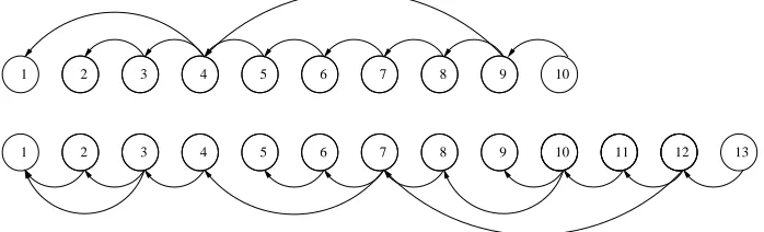
The graphs in Figure 1 represent the direct dependencies between the in-structions in the addition method (top) and the doubling method (bottom). Complete dependency graphs as specified in Definition 2 can be obtained by calculating the transitive closure over the graphs in Figure 1.
Algorithm3 shows a solution for this instance of the optimization problem. The cost of the solution is 12 since we add an extra square and two extra
addi-tions both denoted by the use ofλd as their arguments. It is easy to see that it
is actually an absolute minimal value. To clarify the criteria specified in Defini-tion 5, let us see how they apply to this case.
The pattern Π is given by the operation sequence of the doubling method,
and we have |Π| = 13. To ensure both |F0
1| = 0 (mod|Π|) and |F20| = 0
(mod |Π|) we need to add three dummy instructions toF1. The solution presents
no mismatches between the instruction sequences of either function and the pat-ternΠ, so the restrictionFi0[j] =Π[mod(j,|Π|) + 1] holds for all valid iand j
values. Finally, it is easy to see that both Fi0 are valid transformations of the
originalFi. Instruction reordering occurs only once inF10 (instructions 3 and 5),
and these are independent in F1.F0
2 is identical to F2.
1 2 3 4 5 6 7 8 9 10
1 2 3 4 5 6 7 8 9 10 11 12 13
Fig. 1.Dependency graphs for the methods in Algorithm 2.
3
An Optimisation Algorithm
Algorithm 3Indistinguishable versions of the methods in Algorithm 2.
Input: P = (x1, y1), Q= (x2, y2) Output: R= (x3, y3) =P+Q
1: λd←λ
2
d
2: λd←λd+λd
3: λ2←x2−x1 4: λd←λd+λd
5: λ1←y2−y1 6: λ3←λ−
1 2 7: λ4←λ1·λ3 8: λ5←λ
2 4 9: λ6←λ5−x1 10: x3←λ6−x2 11: λ7←x1−x3 12: λ8←λ4·λ7 13: y3←λ8−y1
Input: P = (x1, y1)
Output: R= (x3, y3) = 2·P 1: λ1←x
2 1 2: λ2←λ1+λ1 3: λ3←λ2+λ1 4: λ4←λ3+A 5: λ5←y1+y1 6: λ6←λ−
1 5 7: λ7←λ4·λ6 8: λ8←λ
2 7 9: λ9←x1+x1 10: x3←λ8−λ9 11: λ10←x1−x3 12: λ11←λ10·λ7 13: y3 ←λ11−y1
but to find a good enough approximation of it that can be used in practical applications.
Algorithm 4 makes S attempts to find an optimal pattern size, which is
selected randomly in each s-iteration (line 2). In each of these attempts, the
original functions are taken as the starting solution, with the minor change that they are padded with dummy instructions, so as to make their size multiple of the pattern size (lines 3 to 6).
The inner loop (lines 10 to 18), which runsT times, uses a set of randomised
heuristics to obtain a neighbour solution. This solution is accepted if it does not represent a relative cost increase greater than the current threshold value. The threshold varies witht, starting at a larger value for low values oftand gradually
decreasing. The number of iterationsS andT must be adjusted according to the
size of the problem.
Π[1] Π[2] ... Π[|Π| −1] Π[|Π|]
2 6 6 6 6 6 6 6 6 6 6 6 4
F0
1[1] F10[2] ... F10[|Π| −1] F10[|Π|] F0
1[|Π|+ 1] F10[2] ... F10[2|Π| −1] F10[2|Π|] ..
. ... ... ... ...
F0
1[|F10| − |Π|+ 1] F10[|F10| − |Π|+ 2] ... F10[|F10| −1] F10[|F10|] F0
2[1] F20[2] ... F20[|Π| −1] F20[|Π|] ..
. ... ... ... ...
F0
N[|FN0 | − |Π|+ 1]FN0 [|FN0 | − |Π|+ 2]... FN0[|FN0| −1] FN0 [|FN0|]
3 7 7 7 7 7 7 7 7 7 7 7 5
Algorithm 4An optimisation algorithm for indistinguishable operations.
Input: (P, ω)
Output: (Π, F0), a quasi-optimal solution to the problem in Definition 5
1: fors= 1 toS do
2: |Π| ←random pattern size 3: x← {Fi,1≤i≤N}
4: for allF0
i ∈x do
5: Append|Π| −(|F0
i| (mod|Π|)) dummy instructions toFi0
6: end for 7: cost←cost(x) 8: result←x 9: best←cost 10: for t= 1 toT do 11: x0←neighbour(x)
12: thresh←threshold(t, T) 13: cost0←cost(x0)
14: if (cost0−cost)/cost−1< threshthen
15: x←x0
16: cost←cost0
17: end if 18: end for
19: if cost < bestthen 20: result←x 21: best←cost 22: end if 23: end for 24: returnresult
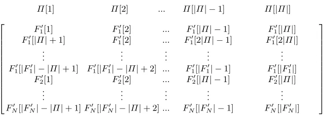
The quality of a solution is measured using a cost function that operates as follows:
– The complete set of instructions in a solutionxis seen as a matrix with|Π|
columns and (PNi=1|F
0
i|)/|Π| lines (see Figure 2), in which each function
occupies|F0
i|/|Π|consecutive lines.
– Throughout the algorithm, the patternΠ is adjusted to each solution by
takingΠ[k] as the most common basic instruction in columnkof the matrix.
– A dummy instruction is always taken to be of the same type as the pattern
instruction for its particular column, so dummy instructions are ignored
when adjustingΠ to a particular solution.
– The overall cost of a solution has two components: c and d. The former
– The relative importance of these components can be tuned to put more or less emphasis on indistinguishability. This affects the trade-off between indistinguishability and processing overhead.
Throughout its execution, the algorithm keeps track of the best solution it has been able to reach (lines 19 to 22); this is returned when the algorithm terminates (line 24).
A neighbour solution is derived from the current solution by randomly se-lecting one of the following heuristics:
Tilt function left A functionF0
i is selected randomly, and its instructions are
all moved as far to the left as possible, filling spaces previously occupied by dummy instructions or just freed by moving other instructions. The order of the instructions is preserved, and an instruction is only moved if it matches the pattern instruction for the target column.
Tilt function right Same as previous, only that instructions are shifted to the right.
Move instruction left A functionF0
i is selected randomly, and an instruction
F0
i[j] is randomly picked within it. This instruction is then moved as far to
the left as possible. An instruction is only moved if this does not violate inter-instruction dependencies, and it matches the pattern instruction for the target column.
Move instruction right Same as previous, only that the instruction is shifted to the right.
After application of the selection heuristic, the neighbour solution is optimised by removing rows or columns containing only dummy instructions. If the final solution produced by Algorithm 4 includes deviations from the chosen pattern, these can be eliminated by extending the pattern to get a totally indistinguish-able result. If the number of mismatches is large, this produces a degenerate solution. We have implemented this as an optional post-processing functionality. Our experimental results indicate the following rules of thumb that should be considered when parameterising Algorithm 4:
– S should be at least half of the length of the longest function.
– T should be a small multiple of the total number of instructions.
– An overall cost function calculated as c2
+d leads to a good compromise
between indistinguishability and processing overhead.
– The threshold should decrease quadratically, starting at 70% fort= 0 and
reaching 10% whent=T−1.
– The neighbour generation heuristics should be selected with equal
probabil-ity, or with a small bias favoring moving over tilting mutations.
4
Results
to construct indistinguishable versions of the much larger functions for point addition and doubling in genus 2 hyper-elliptic curves over finite fields.
Appendix 1 contains the results produced by Algorithm 4 when fed with the
instruction sequences for vanilla EC affine point addition overFpusing projective
coordinates, as presented by Gebotys and Gebotys in (Figure 1,[11]). This result has exactly the same overhead as the version presented in the same reference.
Appendix 2 contains the instruction sequences corresponding to formulae for finite field arithmetic in a specific degree six extension as used in a number of torus based constructions [12, 10], together with the results obtained using Algorithm 4 for this problem instance.
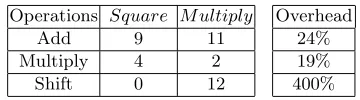
Table 1 (left) shows the number of dummy field operations added to each of the functions in Appendix 2. Also shown in Table 1 (right) is the estimated overhead for an exponentiation. We assume the average case in which the number of squarings is twice the number of multiplications. This is roughly equivalent to the best hand-made solution that we were able to produce in reasonable time, even if the number of dummy multiplications is slightly larger in the automated version.
Table 1.Overheads for the indistinguishable functions in Appendix 2.
Operations Square M ultiply
Add 9 11
Multiply 4 2
Shift 0 12
Overhead 24% 19% 400%
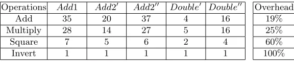
Appendix 3 includes indistinguishable versions of hyper-elliptic curve point adding and doubling functions. These implementations correspond to the general case of the explicit formulae for genus 2 hyperelliptic curves over finite fields using affine coordinates. provided by Lange in [16]. A pseudo-code implementation of these formulae is also included in Appendix 3. In our analysis, we made no assumptions as to the values of curve parameters because our objective was to work over a relatively large problem instance. Operations involving curve parameters were treated as generic operations.
In this example, the group operations themselves contain branching instruc-tions. To accommodate this, we had to first create indistinguishable versions of the smaller branches inside the addition and doubling functions, separately. The process was then applied globally to the two main branches of the addition function and to the doubling function as a whole, which meant processing three functions of considerable size, simultaneously.
Table 2 (left) shows the number of dummy field operations added to each of
the functions in Appendix 3. Note that functionsAdd20 andDouble0 correspond
number of doublings is twice the number of additions, and consider only the
most likely execution sequences for these operations (Add20 andDouble0).
Table 2.Overheads for the indistinguishable functions in Appendix 3.
Operations Add1 Add20 Add200 Double0 Double00
Add 35 20 37 4 16
Multiply 28 14 27 5 16
Square 7 5 6 2 4
Invert 1 1 1 1 1
Overhead 19% 25% 60% 100%
5
Conclusion
Defense against side-channel attacks is a vital part of engineering software that is to be executed on constrained devices. Since such devices are used within an adversarial environment, sound and efficient techniques are of value even if they are hard to implement. To this end we have investigated an automated approach to constructing indistinguishable functions, a general method of defense against certain classes of side-channel attack which are notoriously difficult to implement as the functions grow more complex. Our results show that efficient versions of such functions, which are competitive with hand-constructed versions, can be generated with only minor computational effort.
This work is pitched in the context of cryptography-aware compilation: the idea that programmers should be assisted in describing secure software just like they are offered support to optimise software. We have embedded our algorithm in such a compiler which can now automatically manipulate a source program so the result is more secure.
References
1. D. Agrawal, B. Archambeault, J.R. Rao and P. Rohatgi. The EM Side-Channel(s). InCryptographic Hardware and Embedded Systems (CHES), Springer-Verlag LNCS 2523, 29–45, 2002.
2. D. Agrawal, J.R. Rao and P. Rohatgi. Multi-channel Attacks. InCryptographic Hardware and Embedded Systems (CHES), Springer-Verlag LNCS 2779, 2–16, 2003.
3. I.F. Blake, G. Seroussi and N.P. Smart. Elliptic Curves in Cryptography. Cam-bridge University Press, 1999.
4. I.F. Blake, G. Seroussi and N.P. Smart. Advances in Elliptic Curve Cryptography. Cambridge University Press, 2004.
5. ´E. Brier and M. Joye. Weierstraß Elliptic Curves and Side-channel Attacks. In Public Key Cryptography (PKC), Springer-Verlag LNCS 2274, 335–345, 2002. 6. B. Chevallier-Mames, M. Ciet and M. Joye. Low-Cost Solutions for Preventing
7. J-S. Coron. Resistance against Differential Power Analysis for Elliptic Curve Cryp-tosystems. InCryptographic Hardware and Embedded Systems (CHES), Springer-Verlag LNCS 1717, 292–302, 1999.
8. P. Crescenzi and V. Kann. A Compendium of NP Optimization Problems. Avail-able at: http://www.nada.kth.se/∼viggo/problemlist/.
9. G. Dueck and T. Scheuer. Threshold Accepting: A General Purpose Optimization Algorithm Appearing Superior to Simulated Annealing. InJournal of Computa-tional Physics, 90(1), 161–175, 1990.
10. M. van Dijk, R. Granger, D. Page, K. Rubin, A. Silverberg, M. Stam and D. Woodruff. Practical Cryptography in High Dimensional Tori To appear in Ad-vances in Cryptology (EUROCRYPT), 2005.
11. C.H. Gebotys and R.J. Gebotys. Secure Elliptic Curve Implementations: An Anal-ysis of Resistance to Power-Attacks in a DSP Processor. InCryptographic Hardware and Embedded Systems (CHES), Springer-Verlag LNCS 2523, 114–128, 2002. 12. R. Granger, D. Page and M. Stam. A Comparison of CEILIDH and XTR. In
Algorithmic Number Theory Symposium (ANTS), Springer-Verlag LNCS 3076, 235–249, 2004.
13. M. Joye and J-J. Quisquater. Hessian Elliptic Curves and Side-Channel Attacks. In Cryptographic Hardware and Embedded Systems (CHES), Springer-Verlag LNCS 2162, 402–410, 2001.
14. P.C. Kocher. Timing Attacks on Implementations of Diffie-Hellman, RSA, DSS, and Other Systems. InAdvances in Cryptology (CRYPTO), Springer-Verlag LNCS 1109, 104–113, 1996.
15. P.C. Kocher, J. Jaffe and B. Jun. Differential Power Analysis. InAdvances in Cryptology (CRYPTO), Springer-Verlag LNCS 1666, 388–397, 1999.
16. T. Lange. Efficient Arithmetic on Genus 2 Hyperelliptic Curves over Finite Fields via Explicit Formulae. InCryptology ePrint Archive, Report 2002/121, 2002. 17. P-Y. Liardet and N.P. Smart. Preventing SPA/DPA in ECC Systems Using the
Ja-cobi Form. InCryptographic Hardware and Embedded Systems (CHES), Springer-Verlag LNCS 2162, 391–401, 2001.
18. S.S. Muchnick. Advanced Compiler Design and Implementation, Morgan Kauf-mann, 1997.
19. D. Page and M. Stam. On XTR and Side-Channel Analysis. InSelected Areas in Cryptography (SAC), Springer-Verlag LNCS 3357, 54–68, 2004.
Appendix 1: Arithmetic Over Elliptic Curves Over
F
pUsing Projective Coordinates
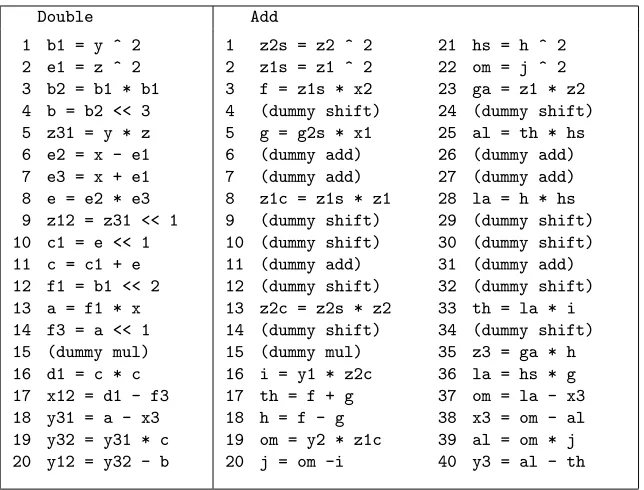
Figure 3 shows the results produced by Algorithm 4 when fed with the
in-struction sequences for vanilla EC affine point addition overFp using projective
coordinates, as presented by Gebotys and Gebotys in (Figure 1,[11]).
Double Add
1 2 3 4 5 6 7 8 9 10 11 12 13 14 15 16 17 18 19 20
b1 = y ^ 2 e1 = z ^ 2 b2 = b1 * b1 b = b2 << 3 z31 = y * z e2 = x - e1 e3 = x + e1 e = e2 * e3 z12 = z31 << 1 c1 = e << 1 c = c1 + e f1 = b1 << 2 a = f1 * x f3 = a << 1 (dummy mul) d1 = c * c x12 = d1 - f3 y31 = a - x3 y32 = y31 * c y12 = y32 - b
1 2 3 4 5 6 7 8 9 10 11 12 13 14 15 16 17 18 19 20
z2s = z2 ^ 2 z1s = z1 ^ 2 f = z1s * x2 (dummy shift) g = g2s * x1 (dummy add) (dummy add) z1c = z1s * z1 (dummy shift) (dummy shift) (dummy add) (dummy shift) z2c = z2s * z2 (dummy shift) (dummy mul) i = y1 * z2c th = f + g h = f - g om = y2 * z1c j = om -i
21 22 23 24 25 26 27 28 29 30 31 32 33 34 35 36 37 38 39 40
hs = h ^ 2 om = j ^ 2 ga = z1 * z2 (dummy shift) al = th * hs (dummy add) (dummy add) la = h * hs (dummy shift) (dummy shift) (dummy add) (dummy shift) th = la * i (dummy shift) z3 = ga * h la = hs * g om = la - x3 x3 = om - al al = om * j y3 = al - th
Appendix 2: Arithmetic Over a Specific a Degree Six
Extension of a Finite Field
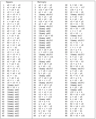
Figure 4 shows the instruction sequences corresponding to formulae for finite field arithmetic in a specific degree six extension, as used in a number of torus based constructions [12, 10]. Figure 5 shows the results obtained using Algorithm 4 for the functions in Figure 4.
Square Multiply 1 2 3 4 5 6 7 8 9 10 11 12 13 14 15 16 17 18 19 20 21 22 23 24 25 26 27 28 29 30 31 32 33 34 35
a0 = x0 - x3 a1 = a0 + x0 c = x3 * a1 c0 = c + a0 c0 = c0 << 1 X4 = c0 + c a1 = x0 + x3 c = a0 * a1 c0 = c + x0 c0 = c0 << 1 X1 = c0 + c a0 = x1 - x4 a1 = x0 - x4 c = x1 * a1 c0 = c + a0 c0 = c0 << 1 X3 = c0 + c a1 = x1 + a0 a1 = - a1 c = x4 * a1 c0 = c + x1 c0 = c0 << 1 X0 = c0 + c a0 = x2 - x5 a1 = a0 - x5 c = x2 * a1 c0 = c - x2 c0 = c0 << 1 X5 = c0 + c a1 = a0 + x2 a1 = - a1 c = x5 * a1 c0 = c - x5 c0 = c0 << 1 X2 = c0 + c
1 2 3 4 5 6 7 8 9 10 11 12 13 14 15 16 17 18 19 20 21 22 23 24 25 26 27 28 29 30 31 32 33 34 35 36
a0 = x0 - x3 b0 = y0 - y3 c12 = a0 * b0 a1 = x1 - x4 b1 = y1 - y4 c13 = a1 * b1 a2 = x2 - x5 b2 = y2 - y5 c14 = a2 * b2 c0 = x0 * y0 c = c13 + c14 t0 = c + c12 t1 = c + c0 t2 = c0 + c14 c8 = x5 * y5 c = c8 + c12 t5 = c + c13 c7 = x4 * y4 c6 = x3 * y3 t4 = c + c7 c = c6 + c7 t3 = c + c14 c1 = x1 * y1 t2 = t2 + c1 a = x0 - x1 b = y0 - y1 c3 = a * b t2 = t2 - c3 t5 = t2 - t5 a = a1 - a2 b = b1 - b2 c17 = a * b t1 = t1 - c17 t4 = t1 - t4 a = a0 - a2 b = b0 - b2
37 38 39 40 41 42 43 44 45 46 47 48 49 50 51 52 53 54 55 56 57 58 59 60 61 62 63 64 65 76 77 78 79 70 71
c16 = a * b t0 = t0 - c16 t3 = t0 - t3 c2 = x2 * y2 c = c + c2 t2 = t2 - c c = c2 + c1 t1 = t1 - c t1 = t1 - c6 c = c + c0 t0 = t0 - c a = x0 - x2 b = y0 - y2 c4 = a * b X0 = t0 + c4 a = x1 - x2 b = y1 - y2 c5 = a * b X1 = t1 + c5 a = x3 - x4 b = y3 - y4 c9 = a * b X2 = t2 + c9 a = x3 - x5 b = y3 - y5 c10 = a * b X3 = t3 + c10 a = x4 - x5 b = x4 - x5 c11 = a * b X4 = t4 + c11 a = a0 - a1 b = b0 - b1 c15 = a * b X5 = t5 + c15
Square Multiply 1 2 3 4 5 6 7 8 9 10 11 12 13 14 15 16 17 18 19 20 21 22 23 24 25 26 27 28 29 30 31 32 33 34 35 36 37 38 39 40 41 42 43 44 45 46 47 48
a0 = x0 - x3 a1 = a0 + x0 c = x3 * a1 c0 = c + a0 c0 = c0 << 1 X4 = c0 + c a1 = x0 + x3 c = a0 * a1 c0 = c + x0 c0 = c0 << 1 X1 = c0 + c a0 = x1 - x4 a1 = x0 - x4 c = x1 * a1 c0 = c + a0 c0 = c0 << 1 X3 = c0 + c a1 = x1 + a0 a1 = - a1 c = x4 * a1 c0 = c + x1 c0 = c0 << 1 X0 = c0 + c a0 = x2 - x5 a1 = a0 - x5 c = x2 * a1 c0 = c - x2 c0 = c0 << 1 X5 = c0 + c a1 = a0 + x2 a1 = - a1 c = x5 * a1 c0 = c - x5 c0 = c0 << 1 (dummy mul) X2 = c0 + c (dummy add) (dummy mul) (dummy add) (dummy add) (dummy add) (dummy mul) (dummy add) (dummy add) (dummy add) (dummy add) (dummy mul) (dummy add) 1 2 3 4 5 6 7 8 9 10 11 12 13 14 15 16 17 18 19 20 21 22 23 24 25 26 27 28 29 30 31 32 33 34 35 36 37 38 39 40 41 42 43 44 45 46 47 48
a0 = x0 - x3 b0 = y0 - y3 c12 = a0 * b0 a1 = x1 - x4 (dummy shift) b1 = y1 - y4 b2 = y2 - y5 c13 = a1 * b1 a2 = x2 - x5 (dummy shift) (dummy add) (dummy add) (dummy add) c14 = a2 * b2 (dummy add) (dummy shift) (dummy add) (dummy add) (dummy add) c0 = x0 * y0 c = c13 + c14 (dummy shift) t2 = c0 + c14 t1 = c + c0 (dummy add) c8 = x5 * y5 a = x0 - x1 (dummy shift) c = c8 + c12 b = y0 - y1 (dummy add) c7 = x4 * y4 t4 = c + c7 (dummy shift) c6 = x3 * y3 c = c6 + c7 t3 = c + c14 c1 = x1 * y1 t2 = t2 + c1 t0 = c + c12 (dummy add) c3 = a * b a = a1 - a2 t2 = t2 - c3 t5 = c + c13 b = b1 - b2 c17 = a * b a = a0 - a2
49 50 51 52 53 54 55 56 57 58 59 60 61 62 63 64 65 66 67 68 69 70 71 72 73 74 75 76 77 78 79 80 81 82 83 84 85 86 87 88 89 90 91 92 93 94 95 96
b = b0 - b2 t1 = t1 - c17 c16 = a * b t5 = t2 - t5 (dummy shift) a = x0 - x2 b = y0 - y2 c2 = x2 * y2 t4 = t1 - t4 (dummy shift) t0 = t0 - c16 c = c + c2 t2 = t2 - c (dummy mul) c = c2 + c1 (dummy shift) t1 = t1 - c t1 = t1 - c6 c = c + c0 c4 = a * b t0 = t0 - c (dummy shift) b = y1 - y2 a = x1 - x2 t3 = t0 - t3 c5 = a * b X0 = t0 + c4 (dummy shift) a = x3 - x4 b = y3 - y4 X1 = t1 + c5 c9 = a * b a = x3 - x5 (dummy shift) (dummy mul) b = y3 - y5 (dummy add) c10 = a * b X3 = t3 + c10 a = x4 - x5 b = x4 - x5 c11 = a * b X2 = t2 + c9 X4 = t4 + c11 a = a0 - a1 b = b0 - b1 c15 = a * b X5 = t5 + c15
Appendix 3: Arithmetic over Genus 2 Hyperelliptic Curves
Over Finite Fields Over Finite Fields
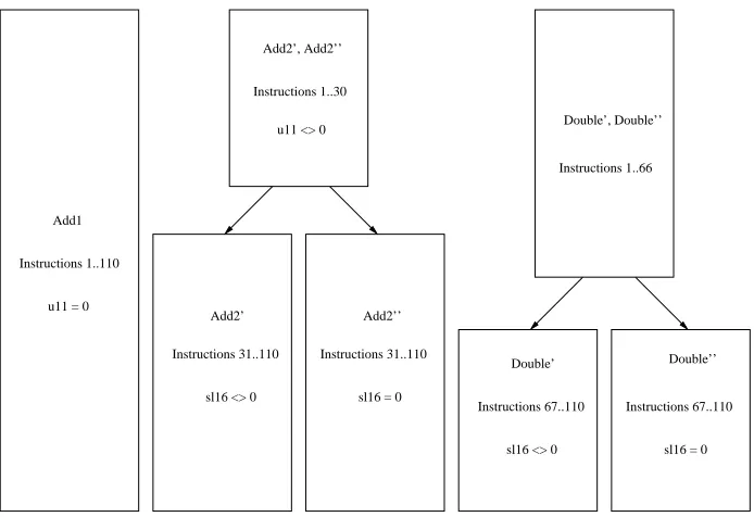
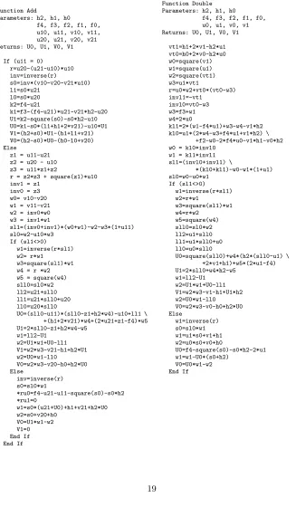
Figures 8 and 9 show indistinguishable versions of hyper-elliptic curve point adding and doubling functions. These implementations correspond to the explicit formulae for genus 2 hyperelliptic curves over finite fields provided by Lange in [16]. Figure 7 contains a pseudo-code implementation of these formulae.
Figure 6 clarifies the relationship between Figures 7, 8 and 9. Note that
vari-ablesl1in the pseudo-code implementation becomes variablesl16in Figures 8
and 9. Note also that, whatever the execution path that occurs, indistinguisha-bility is maintained accross all possible variants.
Add1
Instructions 1..110
u11 = 0
Add2’
Instructions 31..110
Add2’’
Instructions 31..110
sl16 <> 0 Instructions 67..110
sl16 = 0 Instructions 67..110
Double’’ Add2’, Add2’’
Instructions 1..30
u11 <> 0
sl16 = 0 sl16 <> 0
Double’
Instructions 1..66 Double’, Double’’
Fig. 7.Arithmetic on genus 2 hyperelliptic curves over finite fields
Function Add
Parameters: h2, h1, h0
f4, f3, f2, f1, f0, u10, u11, v10, v11, u20, u21, v20, v21 Returns: U0, U1, V0, V1
If (u11 = 0) r=u20-(u21-u10)*u10 inv=inverse(r)
s0=inv*(v10-v20-v21*u10) l1=s0*u21
l0=s0*u20 k2=f4-u21
k1=f3-(f4-u21)*u21-v21*h2-u20 U1=k2-square(s0)-s0*h2-u10 U0=k1-s0*(l1+h1+2*v21)-u10*U1 V1=(h2+s0)*U1-(h1+l1+v21) V0=(h2-s0)*U0-(h0-l0+v20) Else
z1 = u11-u21 z2 = u20 - u10 z3 = u11*z1+z2
r = z2*z3 + square(z1)*u10 inv1 = z1
inv0 = z3 w0= v10-v20 w1 = v11-v21 w2 = inv0*w0 w3 = inv1*w1
sl1=(inv0+inv1)*(w0+w1)-w2-w3*(1+u11) sl0=w2-u10*w3
If (sl1<>0) w1=inverse(r*sl1) w2= r*w1
w3=square(sl1)*w1 w4 = r *w2 w5 = square(w4) sll0=sl0*w2 ll2=u21+sll0 ll1=u21*sll0+u20 ll0=u20*sll0
U0=(sll0-u11)*(sll0-z1+h2*w4)-u10+ll1 \ +(h1+2*v21)*w4+(2*u21+z1-f4)*w5 U1=2*sll0-z1+h2*w4-w5
w1=ll2-U1 w2=U1*w1+U0-ll1 V1=w2*w3-v21-h1+h2*U1 w2=U0*w1-ll0 V0=w2*w3-v20-h0+h2*U0 Else
inv=inverse(r) s0=sl0*w1
*ru0=f4-u21-u11-square(s0)-s0*h2 *ru1=0
w1=s0*(u21+U0)+h1+v21+h2*U0 w2=s0+v20+h0
V0=U1*w1-w2 V1=0 End If End If
Function Double Parameters: h2, h1, h0
f4, f3, f2, f1, f0, u0, u1, v0, v1 Returns: U0, U1, V0, V1
vt1=h1+2*v1-h2*u1 vt0=h0+2*v0-h2*u0 w0=square(v1) w1=square(u1) w2=square(vt1) w3=u1*vt1
r=u0*w2+vt0*(vt0-w3) invl1=-vt1
invl0=vt0-w3 w3=f3+w1 w4=2*u0
kl1=2*(w1-f4*u1)+w3-w4-v1*h2 kl0=u1*(2*w4-w3+f4*u1+v1*h2) \
+f2-w0-2*f4*u0-v1*h1-v0*h2 w0 = kl0*invl0
w1 = kl1*invl1 sl1=(invl0+invl1) \
*(kl0+kl1)-w0-w1*(1+u1) sl0=w0-u0*w1
If (sl1<>0) w1=inverse(r*sl1) w2=r*w1
w3=square(sl1)*w1 w4=r*w2
w5=square(w4) sll0=sl0*w2 ll2=u1+sll0 ll1=u1*sll0+u0 ll0=u0*sll0
U0=square(sll0)+w4*(h2*(sll0-u1) \ +2*v1+h1)+w5*(2*u1-f4) U1=2*sll0+w4*h2-w5
w1=ll2-U1 w2=U1*w1+U0-ll1 V1=w2*w3-v1-h1+U1*h2 w2=U0*w1-ll0 V0=w2*w3-v0-h0+h2*U0 Else
w1=inverse(r) s0=sl0*w1 w1=u1*s0+v1+h1 w2=u0*s0+v0+h0
U0=f4-square(s0)-s0*h2-2*u1 w1=w1-U0*(s0+h2)
Add1 Add20 Add200 Double0 Double00 1 2 3 4 5 6 7 8 9 10 11 12 13 14 15 16 17 18 19 20 21 22 23 24 25 26 27 28 29 30 31 32 33 34 35 36 37 38 39 40 41 42 43 44 45 46 47 48 49 50 51 52 53 54 55 (dummy add) (dummy add) (dummy mul) (dummy add) (dummy add) (dummy mul) (dummy add) (dummy squ) (dummy mul) (dummy add) (dummy add) (dummy add) (dummy squ) (dummy squ) (dummy squ) (dummy mul) (dummy mul) (dummy add) (dummy mul) (dummy add) (dummy mul) (dummy add) (dummy add) (dummy add) (dummy mul) (dummy add) (dummy add) (dummy mul) (dummy add) (dummy add) (dummy mul) (dummy add) (dummy inv) (dummy add) (dummy mul) (dummy add) (dummy squ) (dummy mul) (dummy add) (dummy add) (dummy add) (dummy mul) (dummy add) (dummy mul) (dummy add) (dummy mul) (dummy add) (dummy add) (dummy mul) (dummy add) (dummy add) (dummy mul) (dummy add) (dummy mul) r0 = u21 - u10
z10 = u11 - u21 z20 = u20 - u10 z30 = u11 * z10 z31 = z30 + z20 (dummy add) r0 = z20 * z31 (dummy add) r1 = squ(z10) r2 = r1 * u10 r3 = r2 + r0 w00 = v10 - v20 w10 = v11 - v21 (dummy squ) (dummy squ) (dummy squ) w20 = z31 * w00 w30 = z10 * w10 sl10 = z31 + z10 (dummy mul) sl11 = w00 + w10 sl12 = sl10 * sl11 sl13 = sl12 - w20 sl14 = 1 + u11 (dummy add) sl15 = w30 * sl14 sl16 = sl13 - sl15 (dummy add) sl00 = u10 * w30 sl01 = w20 - sl00 (dummy add) w11 = r3 * sl16 (dummy add) w12 = inv(w11) (dummy add) w21 = r3 * w12 (dummy add) w31 = squ(sl16) sll00 = sl01 * w21 (dummy add) ll20 = u21 + sll00 ul10 = sll00 + sll00 ll10 = u21 * sll00 ul0b = u21 + u21 (dummy mul) ll11 = ll10 + u20 (dummy mul) ul01 = sll00 - z10 ul00 = sll00 - u11 (dummy mul) ul11 = ul10 - z10 ul07 = v21 + v21 w40 = r3 * w21 (dummy add) ul02 = h2 * w40 ul03 = ul01 + ul02
z10 = u11 - u21 z20 = u20 - u10 z30 = u11 * z10 z31 = z30 + z20 (dummy add) r0 = z20 * z31 (dummy add) r1 = squ(z10) r2 = r1 * u10 r3 = r2 + r0 w00 = v10 - v20 w10 = v11 - v21 (dummy squ) (dummy squ) (dummy squ) w20 = z31 * w00 w30 = z10 * w10 sl10 = z31 + z10 (dummy mul) sl11 = w00 + w10 sl12 = sl10 * sl11 sl13 = sl12 - w20 sl14 = 1 + u11 (dummy add) sl15 = w30 * sl14 sl16 = sl13 - sl15 (dummy add) sl00 = u10 * w30 sl01 = w20 - sl00 (dummy add) (dummy mul) (dummy add) inv0 = inv(r3) (dummy add) s00 = sl01 * inv0 (dummy add) ul02 = squ(s00) (dummy mul) (dummy add) ul00 = f4 - u21 ul01 = ul00 - u11 ul04 = s00 * h2 ul03 = ul01 - ul02 (dummy mul) U0 = ul03 - ul04 (dummy mul) (dummy add) w11 = u21 + U0 (dummy mul) w21 = s00 + v20 (dummy add) (dummy mul) (dummy add) w12 = s00 * w11 w13 = w12 + h1
vt10 = v1 + v1 vt11 = h1 + vt10 vt12 = h2 * u1 vt13 = vt11 - vt12 vt00 = v0 + v0 (dummy mul) vt01 = h0 + vt00 (dummy squ) vt02 = h2 * u0 vt03 = vt01 - vt02 (dummy add) (dummy add) w00 = squ(v1) w10 = squ(u1) w20 = squ(vt13) (dummy mul) w30 = u1 * vt13 (dummy add) r0 = u0 * w20 r1 = vt03 - w30 r2 = vt03 * r1 r3 = r0 + r2 invl10 = - vt13 invl00 = vt03 - w30 (dummy mul) w31 = f3 + w10 w40 = u0 + u0 kl10 = f4 * u1 (dummy add) kl11 = w10 - kl10 (dummy mul) kl12 = kl11 + kl11 (dummy inv) kl13 = kl12 + w31 (dummy mul) kl14 = kl13 - w40 (dummy squ) kl15 = v1 * h2 kl16 = kl14 - kl15 kl00 = w40 + w40 kl01 = kl00 - w31 kl02 = f4 * u1 kl03 = kl01 + kl02 kl04 = v1 * h2 kl05 = kl03 + kl04 kl06 = u1 * kl05 kl07 = kl06 + f2 kl08 = kl07 - w00 kl09 = f4 * u0 kl0a = kl09 + kl09 kl0b = kl08 - kl0a kl0c = v1 * h1 kl0d = kl0b - kl0c kl0e = v0 * h2 kl0f = kl0d - kl0e
vt10 = v1 + v1 vt11 = h1 + vt10 vt12 = h2 * u1 vt13 = vt11 - vt12 vt00 = v0 + v0 (dummy mul) vt01 = h0 + vt00 (dummy squ) vt02 = h2 * u0 vt03 = vt01 - vt02 (dummy add) (dummy add) w00 = squ(v1) w10 = squ(u1) w20 = squ(vt13) (dummy mul) w30 = u1 * vt13 (dummy add) r0 = u0 * w20 r1 = vt03 - w30 r2 = vt03 * r1 r3 = r0 + r2 invl10 = - vt13 invl00 = vt03 - w30 (dummy mul) w31 = f3 + w10 w40 = u0 + u0 kl10 = f4 * u1 (dummy add) kl11 = w10 - kl10 (dummy mul) kl12 = kl11 + kl11 (dummy inv) kl13 = kl12 + w31 (dummy mul) kl14 = kl13 - w40 (dummy squ) kl15 = v1 * h2 kl16 = kl14 - kl15 kl00 = w40 + w40 kl01 = kl00 - w31 kl02 = f4 * u1 kl03 = kl01 + kl02 kl04 = v1 * h2 kl05 = kl03 + kl04 kl06 = u1 * kl05 kl07 = kl06 + f2 kl08 = kl07 - w00 kl09 = f4 * u0 kl0a = kl09 + kl09 kl0b = kl08 - kl0a kl0c = v1 * h1 kl0d = kl0b - kl0c kl0e = v0 * h2 kl0f = kl0d - kl0e
Fig. 8. Indistinguishable arithmetic operations for genus 2 hyperelliptic curves over finite fields: instructions 1 to 55. The first three columns correspond to point adding. Add1 is the complete instruction sequence if the (u11 = 0) branch is chosen, Add20
represents the case when the (u11 <> 0∧sl16 <> 0) branches occur, and Add200
corresponds to the (u11<>0∧sl16 = 0) branches. The last two columns correspond point doubling.Double0is the complete instruction sequence if the (sl16<>0) branch
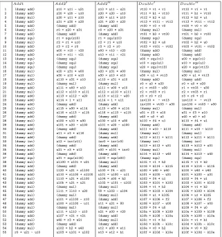
Add1 Add20 Add200 Double0 Double00 56 57 58 59 60 61 62 63 64 65 66 67 68 69 70 71 72 73 74 75 76 77 78 79 80 81 82 83 84 85 86 87 88 89 90 91 92 93 94 95 96 97 98 99 100 101 102 103 104 105 106 107 108 109 110 (dummy mul) r1 = u10 * r0 r2 = u20 - r1 s00 = v10 - v20 (dummy mul) k10 = f4 - u21 (dummy add) s01 = v21 * u10 s02 = s00 - s01 k11 = k10 * u21 k12 = f3 - k11 (dummy mul) inv0 = inv(r2) (dummy mul) (dummy squ) (dummy mul) (dummy mul) (dummy squ) k13 = v21 * h2 k20 = f4 - u21 s03 = s02 * inv0 k14 = k12 - k13 ul12 = s03 * h2 ul10 = squ(s03) ul11 = k20 - ul10 l10 = s03 * u21 (dummy add) vl12 = h1 + l10 vl00 = h2 - s03 (dummy mul) vl10 = h2 + s03 ul13 = ul11 - ul12 U1 = ul13 - u10 ul05 = u10 * U1 ul00 = l10 + h1 vl13 = vl12 + v21 l01 = s03 * u20 (dummy add) (dummy add) k15 = k14 - u20 (dummy mul) ul01 = v21 + v21 ul02 = ul00 + ul01 ul03 = s03 * ul02 vl02 = h0 - l01 ul04 = k15 - ul03 vl11 = vl10 * U1 vl03 = vl02 + v20 (dummy mul) U0 = ul04 - ul05 vl01 = U0 * vl00 (dummy add) V0 = vl01 - vl03 (dummy mul) V1 = vl11 - vl13
w32 = w31 * w12 ul04 = ul00 * ul03 (dummy add) ul05 = ul04 - u10 ll00 = u20 * sll00 (dummy add) ul08 = h1 + ul07 (dummy mul) ul0c = ul0b + z10 ul09 = ul08 * w40 ul0d = ul0c - f4 (dummy mul) (dummy inv) (dummy mul) (dummy squ) (dummy mul) (dummy mul) (dummy squ) (dummy mul) (dummy add) (dummy mul) ul06 = ul05 + ll11 ul12 = h2 * w40 w50 = squ(w40) ul0a = ul06 + ul09 (dummy mul) ul13 = ul11 + ul12 U1 = ul13 - w50 w13 = ll20 - U1 ul0e = ul0d * w50 (dummy add) (dummy add) U0 = ul0e + ul0a w22 = U1 * w13 w23 = w22 + U0 w24 = w23 - ll11 vl10 = w24 * w32 (dummy add) (dummy add) vl11 = vl10 - v21 w25 = U0 * w13 vl12 = vl11 - h1 w26 = w25 - ll00 vl00 = w26 * w32 (dummy add) vl01 = vl00 - v20 (dummy mul) vl02 = vl01 - h0 vl13 = h2 * U1 V1 = vl12 + vl13 vl03 = h2 * U0 (dummy add) (dummy add) (dummy mul) V0 = vl03 + vl02
(dummy mul) (dummy mul) (dummy add) w14 = w13 + v21 w15 = h2 * U0 (dummy add) w16 = w14 + w15 (dummy mul) (dummy add) vl00 = U0 * w16 (dummy add) (dummy mul) (dummy inv) (dummy mul) (dummy squ) (dummy mul) (dummy mul) (dummy squ) (dummy mul) (dummy add) (dummy mul) w22 = w21 + h0 (dummy mul) (dummy squ) V0 = vl00 - w22 (dummy mul) (dummy add) (dummy add) (dummy add) (dummy mul) (dummy add) (dummy add) (dummy add) (dummy mul) (dummy add) (dummy add) (dummy mul) (dummy add) (dummy add) (dummy add) (dummy mul) (dummy add) (dummy add) (dummy mul) (dummy add) (dummy add) (dummy mul) (dummy add) (dummy mul) (dummy add) (dummy mul) (dummy add) (dummy add) (dummy mul) (dummy add)
w01 = kl0f * invl00 w11 = kl16 * invl10 sl10 = invl00+invl10 sl11 = kl0f + kl16 sl12 = sl11 * sl10 sl13 = sl12 - w01 sl14 = 1 + u1 sl15 = sl14 * w11 sl16 = sl13 - sl15 sl00 = u0 * w11 sl01 = w01 - sl00 w12 = r3 * sl16 w13 = inv(w12) w21 = r3 * w13 w32 = squ(sl16) w33 = w32 * w13 w41 = r3 * w21 w50 = squ(w41) sll00 = sl01 * w21 ll20 = u1 + sll00 ll10 = u1 * sll00 ll11 = ll10 + u0 ll00 = u0 * sll00 ul00 = squ(sll00) ul01 = sll00 - u1 ul02 = h2 * ul01 ul03 = v1 + v1 ul04 = ul02 + ul03 ul05 = ul04 + h1 ul06 = w41 * ul05 ul07 = ul00 + ul06 ul08 = u1 + u1 ul09 = ul08 - f4 ul0a = ul09 * w50 U0 = ul07 + ul0a ul10 = sll00 + sll00 ul11 = w41 * h2 ul12 = ul10 + ul11 U1 = ul12 - w50 w14 = ll20 - U1 w22 = U1 * w14 w23 = w22 + U0 w24 = w23 - ll11 vl10 = w24 * w33 vl11 = vl10 - v1 vl12 = vl11 - h1 vl13 = U1 * h2 V1 = vl12 + vl13 w25 = U0 * w14 w26 = w25 - ll00 vl00 = w26 * w33 vl01 = vl00 - v0 vl02 = vl01 - h0 vl03 = h2 * U0 V0 = vl02 + vl03
w01 = kl0f * invl00 w11 = kl16 * invl10 sl10 = invl00+invl10 sl11 = kl0f + kl16 sl12 = sl11 * sl10 sl13 = sl12 - w01 sl14 = 1 + u1 sl15 = sl14 * w11 sl16 = sl13 - sl15 sl00 = u0 * w11 sl01 = w01 - sl00 (dummy mul) w12 = inv(r3) (dummy mul) (dummy squ) (dummy mul) (dummy mul) (dummy squ) s00 = sl01 * w12 (dummy add) w13 = u1 * s00 w14 = w13 + v1 (dummy mul) ul00 = squ(s00) (dummy add) (dummy mul) (dummy add) (dummy add) (dummy add) (dummy mul) (dummy add) (dummy add) (dummy add) (dummy mul) (dummy add) (dummy add) w21 = u0 * s00 w22 = w21 + v0 ul01 = f4 - ul00 (dummy add) (dummy mul) w23 = w22 + h0 ul04 = u1 + u1 ul02 = s00 * h2 (dummy add) ul03 = ul01 - ul02 (dummy mul) U0 = ul03 - ul04 (dummy mul) w16 = s00 + h2 w17 = U0 * w16 w15 = w14 + h1 w18 = w15 - w17 vl00 = U0 * w18 V0 = vl00 - w23
Fig. 9. Indistinguishable arithmetic operations for genus 2 hyperelliptic curves over finite fields: instructions 56 to 110. The first three columns correspond to point adding. Add1 is the complete instruction sequence if the (u11 = 0) branch is chosen, Add20
represents the case when the (u11 <> 0∧sl16 <> 0) branches occur, and Add200
corresponds to the (u11<>0∧sl16 = 0) branches. The last two columns correspond point doubling.Double0is the complete instruction sequence if the (sl16<>0) branch
![Figure 4 shows the instruction sequences corresponding to formulae for finite fieldarithmetic in a specific degree six extension, as used in a number of torus basedconstructions [12, 10]](https://thumb-us.123doks.com/thumbv2/123dok_us/1847105.1239638/16.595.146.470.221.529/instruction-sequences-corresponding-formulae-eldarithmetic-specic-extension-basedconstructions.webp)