econstor
Der Open-Access-Publikationsserver der ZBW – Leibniz-Informationszentrum Wirtschaft
The Open Access Publication Server of the ZBW – Leibniz Information Centre for Economics
Nutzungsbedingungen:
Die ZBW räumt Ihnen als Nutzerin/Nutzer das unentgeltliche, räumlich unbeschränkte und zeitlich auf die Dauer des Schutzrechts beschränkte einfache Recht ein, das ausgewählte Werk im Rahmen der unter
→ http://www.econstor.eu/dspace/Nutzungsbedingungen nachzulesenden vollständigen Nutzungsbedingungen zu vervielfältigen, mit denen die Nutzerin/der Nutzer sich durch die erste Nutzung einverstanden erklärt.
Terms of use:
The ZBW grants you, the user, the non-exclusive right to use the selected work free of charge, territorially unrestricted and within the time limit of the term of the property rights according to the terms specified at
→ http://www.econstor.eu/dspace/Nutzungsbedingungen By the first use of the selected work the user agrees and declares to comply with these terms of use.
zbw
Leibniz-Informationszentrum WirtschaftChristmann, Andreas; Steinwart, Ingo; Hubert, Mia
Working Paper
Robust Learning from Bites for Data
Mining
Technical Report / Universität Dortmund, SFB 475 Komplexitätsreduktion in Multivariaten Datenstrukturen, No. 2006,03
Provided in cooperation with:
Technische Universität Dortmund
Suggested citation: Christmann, Andreas; Steinwart, Ingo; Hubert, Mia (2006) : Robust Learning from Bites for Data Mining, Technical Report / Universität Dortmund, SFB 475 Komplexitätsreduktion in Multivariaten Datenstrukturen, No. 2006,03, http:// hdl.handle.net/10419/22651
Universiteit Leuven 3
Some methods from statistical machine learning and from robust statistics have two drawbacks. Firstly, they are computer-intensive such that they can hardly be used for massive data sets, say with millions of data points. Secondly, robust and non-parametric confidence intervals for the predictions according to the fitted models are often unknown. Here, we propose a simple but general method to over-come these problems in the context of huge data sets. The method is scalable to the memory of the computer, can be distributed on several processors if available, and can help to reduce the computation time substantially. Our main focus is on robust general support vector machines (SVM) based on minimizing regular-ized risks. The method offers distribution-free confidence intervals for the median of the predictions. The approach can also be helpful to fit robust estimators in parametric models for huge data sets.
1. Introduction
Data sets with millions of observations occur nowadays in many areas, e.g. insurance com-panies or banks collect many variables to develop tariffs and scoring methods for credit risk management, respectively. Other examples are large observational data sets in data mining projects and data from micro-arrays. Although such big data sets contain a lot of valuable information, the analysis of such data sets can not only be cumbersome due to computer memory or computational time problems. Classical parametric assumptions are often violated for such data sets which contain probably some outliers. We give only to three citations for these facts. J.W. Tukey, one of the pioneers of robust statistics, mentioned already in 1960 (citet from Hampel et al. (1986, p. 21)): ”A tacit hope in ignoring devi-ations from ideal models was that they would not matter; that statistical procedures which were optimal under the strict model would still be approximately optimal under the approx-imate model. Unfortunately, it turned out that this hope was often drastically wrong; even mild deviations often have much larger effects than were anticipated by most statisticians.”
Le Cam (1980, p.478) concluded for data sets with n= 105 ton= 108 data points: ”Thus
the asymptotics fail precisely when one would feel that they are applicable.” Hampel et al.
(1986, p. 27f) made the following comment on data quality and gross errros. ”There are often no or virtually no gross errors in high-quality data, but 1%to 10% of gross errors in routine data seem to be more the rule than the exception”. Hence, it is no surprise that the
1. Address: University of Dortmund, Department of Statistics, D-44221 Dortmund, GERMANY. 2. Address: Los Alamos National Laboratory, Los Alamos, NM 87545, CCS-3, Mail Stop B256, USA. 3. Address: Katholieke Universiteit Leuven, Department of Mathematics, W. de Croylaan 54, B-3001
Leuven, BELGIUM.
3.AMS 2000 subject classification. Primary 62G08, 62G35; secondary 68Q32, 62G20.
4.Keywords and Phrases. Breakdown point, convex risk minimization, data mining, distributed computing, influence function, logistic regression, robustness, scalability, statistical machine learning, support vector machine.
data quality in large data mining problems is often far from being optimal,cf. Handet al.
(2001) or Hippet al. (2001).
The application of robust statistical methods is therefore important in such situations. Unfortunately, many robust methods proposed in the literature have the following draw-backs which are serious limitations for their application. (a) They are computer-intensive such that they can hardly be used for massive data sets, say for several millions of ob-servations with hundreds of explanatory variables. (b) Robust standard errors and robust confidence intervals for the estimated parameters or for robust predictions are often un-known. (c) Some statistical software packages like S-PLUS or R contain state-of-the-art algorithms for robust statistical methods, but the implemented numerical algorithms usu-ally require that the whole data set fits into the memory of the computer.
In this paper a simple but quite general method for robust estimation in the context of huge data sets is proposed. The main goal of the proposal is to broaden in application of robust general SVM methods for massive data. The idea is to partition the huge data setS
by random into disjoint subsetsSb,b= 1, . . . , B. Then a robust method is applied to each
subset, and the results are summarized in a robust manner. The proposal yields robust predictions. If the median is used to aggregate the B single predictions then we also get robust and distribution-free confidence intervals.
The rest of the paper is organized as follows. Section 2 gives the proposed method and Section 3 describes its properties. Section 4 given some numerical examples for the case of robust linear regression and kernel logistic regression. Section 5 contains a summary and compares RLB with competing methods. All proofs are given in the Appendix.
2. Method
In this section we describe a simple but rather general method for robust estimation for huge data sets. We restrict attention to classification and regression problems although the method can be used in other fields as well. The proposal has two goals: making robust general SVM methods usable for data sets which are too large for currently available algorithms due to memory or time limitations and offering robust and distribution-free confidence intervals based on the median for the predictions.
In classification and in regression problems one assumes an approximate functional re-lationship between an explanatory random variable X and a response random variable Y
using nobservations (xi, yi)∈ X × Y ⊂Rd×Rdrawn independently from the same
prob-ability distribution P of the pair (X, Y). In a non-parametric setting the distribution P is totally unknown. For technical reasons we assume throughout this work thatX andY are closed or open subsets ofRdandR, respectively. Hence we can split up P into the marginal distribution PX and the regular conditional probability P(· |x),x∈ X, on Y. For the case
of binary classification we have Y={−1,+1}.
For regression one often imposes the classical signal plus noise assumption, i.e. the as-sumption thatYi|(X=xi) is distributed asf(xi) +εi, wheref is an unknown function and
εi are independent and identically distributed error terms, 1≤i≤n. In the linear
(para-metric) setup we additionally assume f(x) =fθ(x) = x0θ, θ∈Θ⊂Rd, and in the general
non-parametric setup f is simply a measurable function, i.e. f : (X,B(X))→ (R,B(R)). A possible intermediate case is based on the assumption that f belongs to some Hilbert
space H of all measurable functions f : (X,B(X)) → (R,B(R)). In our case H can be a (typically infinite dimensional) reproducing kernel Hilbert space (RKHS).
We assume that the statistical method of interest can be written as a function of the empirical distribution 1
n
Pn
i=1δ{(xi,yi)} based on the data setS having data points (xi, yi), i= 1, . . . , n.1 Hereδ
{z} denotes the Dirac-distribution in{z}. More general we assume that TPis the quantity of interest for any distribution P, where
T : P7→TP (1)
is a measurable function defined on the space of probability distributionsM(X × Y,B(X × Y)). Examples are the mean TP =EP(X) =
R
XdP (if existent) and the minimizer TP = fP,λ,λ >0, of the regularized theoretical risk defined in (8).
In this paper we always assume that the sample size n is large. The whole data set is often partitioned by random into two or three disjoint parts for training, validation, and testing purposes. Instead of modelling the full training data set, we split the training data set by random into B ≥ 1 parts Sb (called ’bites’) of approximately the same sub-sample
sizes nb ≈ n/B. Then we fit each bite with the robust method. Finally, we compute a
robust location estimator of the estimators TSb and summarize the predictions from theB
fitted models.
Definition 1 Let S = ((x1, y1), . . . ,(xn, yn)) be a sample of size n from a probability dis-tributionP on(X×Y,B(X×Y)). Let TS be the estimator of interest. Consider a random partition ofS into B non-empty subsets, i.e.
S =S1∪. . .∪ SB, (2) where Sb ⊂ S, nb := #Sb ≈ bn/Bc ∈ N, n =
PB
b=1 nB, b = 1, . . . , B, B ∈ {1, . . . , n}, B ¿n. AnRLB estimator of type I is defined by
TSRLB,B =g(TS1, . . . , TSB), (3)
where g:HB →H is a measurable map. An RLB estimator of type IIis given by
TSRLB,B (x) =g∗(TS1(x), . . . , TSB(x)), ∀x∈X, (4)
where g∗:RB →Ris a measurable map.
Remarks. (i) An RLB estimator of type I can obviously be used to define an RLB estimator of type II. (ii) An RLB estimator of type II does not necessarily define an RLB estimator of type I, because the related function g∗ does not necessarily correspond to a
function g mapping onto the Hilbert space H. (iii) The class of RLB estimators of type I
−and due to part (i) the class of RLB estimators of type II−is non-empty, because for g
equal to the mean be obtain: g(TS1, . . . , TSB) := 1
B
PB
b=1TSb ∈H.
1. If misunderstandings are improbable, we will use the symbolSfor the data set and for the corresponding empirical distribution.
We will mainly consider RLB estimators of type I which are convex combinations TSRLB,B = B X b=1 cbTSb (5)
with weights cb ∈(0,1) and
PB
b=1cb = 1 (cb ≡ B1 gives the mean), and RLB estimators of
type II based on the median. Of course, L–estimators such as α-trimmed means, M–, S–, and R–estimators can also be used on the aggregation step.
If B is large enough, say above 15, precision estimates can additionally be obtained by computing standard deviations of the predictionsTRLB
S,B (x) using the central limit theorem.
However, in general we favor a distribution-free method based on the median. IfB is small or if the distribution or the variance ofTRLB
S,B (x) is unknown, one can construct
distribution-free confidence intervals for the median ofTRLB
S,B (x) and distribution-free tolerance regions
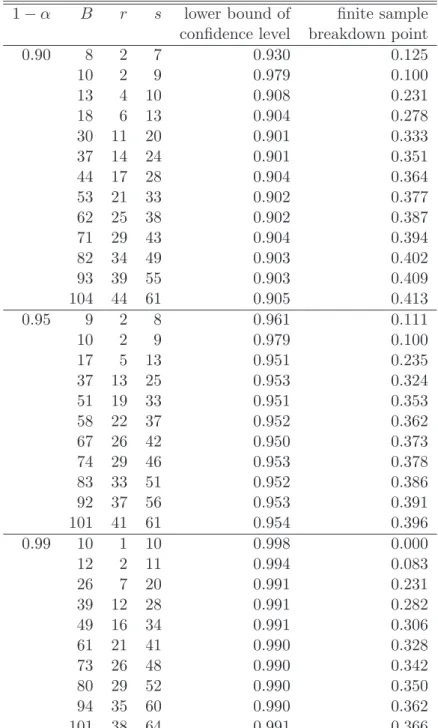
based on selected order statistics, see David and Nagaraja (2003, Chap. 7). Table 1 lists some values of B, the corresponding pair of order statistics determining the confidence interval, the lower bound of the actual confidence level which is 0.5B Ps
j=r(Bj ), and the
finite sample breakdown point ε∗
B = min{r−1, B−s}/B of the confidence interval, see
Definition 10. In Section 3 it will be shown that RLB inherits robustness properties from the original estimator and from the estimator used in the aggregation step. The actual confidence intervals based on the median can be conservative for small choices of B, see Table 1. If B is not too small, sayB >15, this breakdown point is high enough for many practical applications. E.g. fix B = 17. Then the 5th and the 13th order statistics give a
confidence interval at the level 95% for the median which is valid for all distributions on (R,B(R)). The breakdown point of this confidence interval is 4/17 = 0.235 because the values of the four lowest and the four highest predictions are not used.
3. Properties of RLB
In this section properties of robust learning from bites are investigated. Computational time and memory space are considered in Section 3.1. RLB for general SVM estimators is investigated in Section 3.2, and robustness properties are proved in Section 3.3. In Section 3.4 some arguments are given how to choose the number of bites. All proofs are given in the appendix.
We will assume in this section that min1≤b≤Bnb → ∞,n→ ∞.
3.1 General properties
Denote the estimator based on the whole data set by TS and denote the corresponding RLB estimator based onB bites,B fixed, with sub-sample sizesnb, wheren=
PB
b=1nb, by
TRLB
S,B .
The estimators TSb, 1 ≤ b ≤ B, from the bites are stochastically independent because they are computed from disjoint parts of the data set. The computation time and the memory space for RLB can be obviously approximated in the following way. Denote the number of available CPUs bykand letkBbe the smallest integer which is not smaller than
1−α B r s lower bound of finite sample confidence level breakdown point
0.90 8 2 7 0.930 0.125 10 2 9 0.979 0.100 13 4 10 0.908 0.231 18 6 13 0.904 0.278 30 11 20 0.901 0.333 37 14 24 0.901 0.351 44 17 28 0.904 0.364 53 21 33 0.902 0.377 62 25 38 0.902 0.387 71 29 43 0.904 0.394 82 34 49 0.903 0.402 93 39 55 0.903 0.409 104 44 61 0.905 0.413 0.95 9 2 8 0.961 0.111 10 2 9 0.979 0.100 17 5 13 0.951 0.235 37 13 25 0.953 0.324 51 19 33 0.951 0.353 58 22 37 0.952 0.362 67 26 42 0.950 0.373 74 29 46 0.953 0.378 83 33 51 0.952 0.386 92 37 56 0.953 0.391 101 41 61 0.954 0.396 0.99 10 1 10 0.998 0.000 12 2 11 0.994 0.083 26 7 20 0.991 0.231 39 12 28 0.991 0.282 49 16 34 0.991 0.306 61 21 41 0.990 0.328 73 26 48 0.990 0.342 80 29 52 0.990 0.350 94 35 60 0.990 0.362 101 38 64 0.991 0.366
Table 1: Selected pairs (r, s) of order statistics for non-parametric confidence intervals at the (1−α)-level for the median.
Proposition 2 (Computation time, k CPUs) Assume that the computation time ofTS
h is some positive function. Then the computation time of TRLB
S,B with subsample sizes
nb ≈n/B is approximately of order O(kB·h(n/B, d)).
Proposition 3 (Memory space, k CPUs) Assume that the estimatorTS for a data set with n observations and d explanatory variables needs memory space and hard disk space of order O(h1(n, d)) and O(h2(n, d)), respectively, where h1 and h2 are positive functions.
Then the computation of TRLB
S,B for subsample sizes nb ≈n/B needs approximately memory space and hard disk space of order O(k·h1(n/B, d)) andO(k·h2(n/B, d)), respectively. Proposition 4 (Consistency) Consider an RLB estimator TRLB
S,B of type I based on a convex combination with cb ∈(0,1)and PBb=1cb = 1.
(i) IfE(TSb) =E(TS) for allb∈ {1, . . . , B}, then E(T
RLB
S,B ) =E(TS).
(ii) If TS converges in probability (or almost sure) toTP for n→ ∞ and if (n/nb)→B, B fixed, then TRLB
S,B converges in probability (or almost sure) to TP.
(iii) Let cb ≡ B1. Assume that nb1/2(TSb −TP) converges weakly to a multivariate normal
distributionN(0,Σ), whereΣ∈Rd×dis positive definite, and that (n/n
b)→B, 1≤b≤B,
B fixed. Then n1/2(TRLB
S,B −TP) converges weakly to a multivariate normal distribution
N(0,Σ), n→ ∞.
Proposition 5 (Consistency) Consider an RLB estimator TSRLB,B of type II where the
medianis used in the aggregation step. IfTS(x)converges in probability (or almost sure) to TP(x), x∈ X, and if limn→∞ (n/nb)≡B,B fixed, then TSRLB,B (x)converges in probability (or almost sure) toTP(x).
3.2 Properties of RLB using the mean for general SVM methods
Now we consider general SVM estimators
fS,λ:= arg min f∈H 1 n n X i=1 L(yi, f(xi)) +λ||f||2H, (6)
where L : Y ×R → [0,∞) is a convex loss function, i.e. a measurable function which is convex in its second argument, H is the reproducing kernel Hilbert space defined via the kernel k : X × X → R, and regularizing parameter λ > 0, see Vapnik (1998) and Sch¨olkopf and Smola (2002). Special cases of such general SVM methods are the support vector machine: L(y, t) = max{0,1−yt}, y ∈ {−1,+1}, t∈ R, kernel logistic regression:
L(y, t) = ln(1 + exp[−yt]), y∈ {−1,+1}, t∈R, andε-support vector regression: L(y, t) = max{|y−t| −ε,0},y, t∈R, where ε >0 is fixed. The general SVM estimator fSb,λnb(x), x ∈ X, defined as the solution of (6) for bite Sb is a kernel based estimator and can be written as fSb,λnb(x) = nb X i=1 αi,bk(x, xi), i∈ Sb, x∈ X, (7)
whereαi,b ∈R. Ifαi,b6= 0, then (xi, yi) is called a support vector (SV). Obviously, the
min-imization problem (6) can be interpreted as a stochastic approximation of the minmin-imization of the theoretical regularized risk
fP,λ:= arg min
f∈H EPL(Y, f(X)) +λkfk
2
where the minimizerfP,λexists under rather general assumptions onHandL, see e.g. Stein-wart (2005a) and Christmann and SteinStein-wart (2005).
Theorem 6 (RLB for general SVMs) Assume that the estimatorfS,λis a general SVM estimator defined by (6) for the whole data set with n = PBb=1nb observations, B fixed. Consider an RLB estimator of type I based on a convex combination with cb ∈ (0,1) and
PB
b=1cb = 1. Then the RLB estimator is itself a kernel based estimator and can be written as fSRLB,B,(λ nb)(x) = n X i=1 αi,RLBk(x, xi) (9) = X i∈SV(S1)∪...∪SV(SB) αi,RLBk(x, xi), x∈ X, (10) where αi,RLB= PB b=1cbαi,b, i∈ S.
We have αi,RLB =cbαi,b in (10) if all support vectors are different.
Let us now investigate thenumber of support vectors in more detail for the case of pattern recognition, i.e. Y = {−1,+1}. For part (ii) of our next result we need the following quantities. Denote the marginal distribution of X by PX. Let X0 := {x ∈ X; P(1|X = x) = 1/2},Xcont:={x∈ X; PX({x}= 0)}, and let∂2L denote the subdifferential operator
of the loss function L with respect to the second variable. Further, define the set-valued function
FL∗(α) :={t∈R; [αL(1, t) + (1−α)L(−1, t)] = min
s∈R[αL(1, t) + (1−α)L(−1, t)]}, α ∈[0,1],
the set
S ={(x, y)∈ Xcont× Y; 0∈/∂2L(y, FL∗(P(1|X =x)))∩R} ,
and the quantity
SL,P=
(
P(S) if 0∈/ ∂2L(1, FL∗(0.5))∩∂2L(−1, FL∗(0.5))
P(S) +1
2PX(X0∩ Xcont) else,
see Steinwart (2003, p.1082). We also need the notion of a classification calibrated loss function. Such loss functions were called admissible by Steinwart (2003), but we think that the notion of classification calibrated is more precise. A loss function is called classification calibrated if for every α∈[0,1] we have
FL∗(α)⊂[−∞,0) if α <1/2
FL∗(α)⊂(0,∞] if α >1/2.
For more information on this and related concepts we refer to Bartlett et al. (2006) and Steinwart (2005b).
Finally, we need a way to describe the richness of the reproducing kernel Hilbert space
Definition 7 Let X ⊂ Rd be compact and k : X × X → R be a continuous kernel with reproducing kernel Hilbert space H. Then k is universal if H is dense in the space of continuous functionsC(X) equipped withk.k∞.
Now we can formulate the following theorem on the number of support vectors:
Theorem 8 (Number of support vectors) Consider an RLB estimator of type I based on a convex combination with cb ∈ (0,1) and
PB
b=1cb = 1. Under the assumptions of Theorem 6 the RLB estimator has the following properties.
(i) The number of support vectors, i.e. αi,RLB6= 0, of the RLB estimator is given by
#{SV(S1) ∪ . . . ∪ SV(SB)} . (11) (ii) Consider a binary classification problem, i.e. Y = {−1,+1}. Let B be fixed, and consider n:=B ·nb → ∞. Let L be a classification calibrated and convex loss function, k
be a universal kernel and λnb >0 be a sequence of regularization parameters with λnb → 0
and nbλ2nb/|Lλnb|21→ ∞. Then for all Borel probability measures P on (X × Y,B(X × Y))
the RLB-classifier based on (6) with respect to k, L and (λnb) satisfies
Pr∗n
³
S1∪. . .∪ SB ∈(X × Y)n; #SV(fSRLB,B,(λnb))≥(SL,P−ε)n ´
→1. (12)
Here Pr∗n denotes the outer probability measure of Pn in order to avoid measurability con-siderations.
Note that part (ii) of the above result gives for the RLB estimator thesame asymptotical bound for the number of support vectors as the one forB = 1 derived by Steinwart (2003). The result given in (12) has the following interpretation: with probability tending to 1 if the total sample size n =Bnb converges to ∞, but B is fixed, the fraction of support vectors
of the kernel based RLB estimatorfRLB
S,B,(λnb)(x) in a binary pattern recognition problem is
essentially greater than the Bayes risk.
Now we investigate conditions to guarantee that RLB estimators using general SVM estimators are L−risk consistent, i.e. that they are able to learn. If P is a probability distribution on X × Y, the L-risk of a measurable map f : X → R with respect to P is defined by RL,P(f) := Z L(Y, f(X))dP = Z L(y, f(x)) P(dy|x) PX(dx).
The above integral is always defined since L is non-negative and continuous, although it may be infinite. Consider a general SVM estimatorfS,λ defined by (6) for the whole data
set S. The estimatorfS,λn is called L-risk consistent, if
RL,P(fS,λn)→ R ∗ L,P:= inf © RL,P(f) ;f :X →Rmeasurable ª (13) holds in probability forn→ ∞for suitable chosen regularization sequences (λn)n∈N. Several
authors have given conditions to guarantee that general SVM estimators are L−risk con-sistent,cf. Steinwart (2002, 2005a), Zhang (2004), and Christmann and Steinwart (2005).
If fS,λn is L-risk consistent, B ≥ 1 fixed, and limn→∞min1≤b≤Bnb = ∞, we obtain by
Slutzky’s theorem for an RLB estimator of type I based on a convex combination with weightscb ∈(0,1) and PB b=1cb= 1 that B X b=1 cbRL,P(fSb,λnb)→ R ∗ L,P (14)
in probability for n → ∞. The next result gives L-risk consistency of RLB estimators of type I using a convex combination.
Theorem 9 (L−risk consistency) Let fS,λn be an L-risk consistent general SVM
esti-mator based on (6) with a convex loss function. Then the RLB estiesti-mator of type I defined by fSRLB,B,(λ
nb)= PB
b=1cbfSb,λnb with cb ∈(0,1)and PB
b=1cb = 1 isL-risk consistent, i.e.
RL,P Ã B X b=1 cbfSb,λnb ! −→P R∗ L,P, n→ ∞. (15)
From the no-free-lunch theorem by Devroye (Devroyeet al., 1997) our proof given in the appendix can in general not be modified in a simple way to cover the case that the number
B of bites depends on the sample size, because we have no uniform rate of consistency without restricting the class of probability distributions, see also Tsybakov (2004).
3.3 Robustness properties of RLB
Now we derive results which show that certain robustness properties are inherited from the original estimator TS to the RLB estimator. We will restrict attention to two robustness
approaches. The finite sample breakdown point proposed by Donoho and Huber (1983) mea-sures the worst case behavior of a statistical estimator. Then influence function proposed by Hampel (1968, 1974), measures the impact on the estimation due to an infinitesimal small contamination of the distribution P in direction of a Dirac-distribution.
Definition 10 (Finite-sample breakdown point) Let Sn={(xi, yi), i= 1, . . . , n} be a data set with values in X × Y. The finite-sample breakdown point of an estimator TSn is defined by ε∗n(TSn) = min nm n ; Bias(m;TSn) is finite o , (16) where Bias(m;TSn) = sup S0 n kTS0 n−TSn k (17)
and the supremum is over all possible samples S0
n that can be obtained by replacing any m of the original data points by arbitrary values in X × Y.
Theorem 11 (Finite-sample breakdown point of RLB) Consider RLB withB bites wherenb ≡n/B. Denote the finite sample breakdown point of the estimatorTSb for bitebby
in the aggregation step by ε∗
B(ˆµ). Then the finite sample breakdown point of the RLB estimator is given by ε∗RLB,S,B = 1 n à k X b=1 ¡ nbε∗nb(TSb) + 1 ¢ (b:B)−1 ! , (18)
where k is the smallest integer not less than Bε∗
B(ˆµ) + 1 and z(1:B) ≤. . . ≤z(B:B) denote
the ordered values of {z1, . . . , zB}.
Remark. If all values nbε∗
nb(TSb) are equal, we obtain ε∗RLB,S,B = ¡ nbε∗ nb(TSb) + 1 ¢ dBε∗ B(ˆµ) + 1e −1 n ≥ε ∗ nb(TSb)ε ∗ B(ˆµ). (19)
If the mean or any other estimator withε∗B(ˆµ) = 0 is used in this situation, then the RLB has a finite sample breakdown point ofε∗
nb(TSb)/B→0, if B → ∞. HenceB should not be
too large.
Example 12 (Univariate location model) Consider the univariate location problem, where xi ≡1 andyi ∈R, i= 1, . . . , n, n= 55. Assume that yi 6=yj fori6=j. The finite
sample breakdown point of the median is [[n/2]]/n = 0.49. The mean has a finite sample breakdown point of 0. Let us investigate the robustness of RLB withB = 5 and nb = 11,
b = 1, . . . , B. (a) If the median is used as the location estimator in each bite and if the median is used in the aggregation step, then ε∗
RLB,Sn,B = 0.309. This value is reasonably
high, but lower than the finite sample breakdown point of the median for the whole data set. Note that in afortunate situation the impact of up to (2×11 + 5×3)/55 = 0.672 extreme large data points (say with values equal to +∞) is still bounded for the RLB estimator in this setup: modify all data points in Bε∗B(ˆµ) = 2 bites and up to nbε∗nb(TSb) = 5
data points in the remaining B(1−ε∗
B(ˆµ)) = 3 bites. This is no contradiction because
the breakdown point measures the worst case behavior. (b) If the median is used as the location estimator in each bite and if the mean is used in the aggregation step, then we obtain ε∗
RLB,Sn,B = (1/B)ε ∗
nb(TSb) = 0.09. (c) If the mean is used as the location estimator
in each bite and also in the aggregation step we haveε∗
RLB,Sn,B = 0. ¢
Now we investigate the influence function of an RLB estimator TRLB
S,B =
PB
b=1cbTSb of
type I with weights cb ∈(0,1) and PBb=1cb = 1.
To this end we assume the existence of a mapT which assigns to every distribution P on a given setZ an elementT(P) of a given Banach spaceE such that our RLB estimator for a data setS =S1∪. . .∪SB has the representation
TSRLB,B =
B
X
b=1
cbT(PSb). (20)
Here PSb denotes the empirical distribution of the data points in bite Sb,b= 1, . . . , B. We
have T(P) = θ∈ E =Rd for parametric models and E =H and T(P) =f
P,λ for general
Definition 13 (Influence function) The influence function of T at a point z for a dis-tribution P is the special Gˆateaux derivative (if it exists)
IF(z;T,P) = lim ε↓0 T¡(1−ε)P +εδz ¢ −T(P) ε , (21)
where δz is the Dirac distribution at the point z such that δz({z}) = 1.
The influence function has the interpretation, that it measures the impact of an (in-finitesimal) small amount of contamination of the probability distribution P in direction of a Dirac distribution located in the point {z} on the theoretical quantity of interest T(P). Therefore, in the robustness approach based on influence functions it is desirable that a statistical method which can be written as T(P) has abounded influence function.
Theorem 14 (Influence function of RLB) Assume that the original estimator TS has the representation T(Pn), where Pn is the empirical distribution of the sample S, and that the influence function of the map T(P) exists for the probability distribution P. Then the RLB estimator of type I using the weights cb ∈(0,1)and
PB
b=1cb = 1 with a fixed number
B of bites and n/nb ≡B exists and equals the influence function of T(P).
Hence, ifT(P) has a bounded influence function, the same is true for RLB. The influence function is one of the cornerstones of robust statistics. Many robust estimators in para-metric statistical methods have a bounded influence function, see e.g. Hampelet al.(1986) for M-estimators and GM-estimators and Davies (1990, 1993) for S-estimators. Recently, Christmann and Steinwart (2004, 2005) showed that the influence function of many gen-eral SVM methods exists for the case of classification and regression. Further the influence function of such methods is bounded if a loss functionLwith bounded first derivative and a bounded and universal kernelkare used. An example is kernel logistic regression in combi-nation with a Gaussian radial basis function kernelk(x, x0) = exp(−γ||x−x0||2),x, x0 ∈ X,
whereγ ∈(0,∞).
3.4 Determination of the number B of bites
From the results given in Sections 3.1 to 3.3 it is obvious, that the number of bites has some impact on the statistical behavior of the RLB estimator and also on the computation time and the necessary computer memory. An optimal choice of the numberB of bites will in general depend on the unknown distribution P. But some informal arguments are given how to determineB in an appropriate manner.
One should take the sample size n, the computer resources (number of CPUs, RAM) and the acceptable computation time into account. The quantity B should be much lower than n, because otherwise there is not much hope to obtain useful estimators from the bites and because the finite sample breakdown point is generally decreasing with increasing values of B. Further, B should depend on the dimensionality dof the explanatory vectors
xi ∈ X. E.g. a rule of thump for linear regression is that n/d should be at least 5.
Because the functionf is completely unknown in nonparametric regression assumptions on the complexity off are crucial. The sample sizenb for each bite should converge to infinity, ifn→ ∞, to obtain consistency of RLB. The results from some numerical experiments not
given here can be summarized as follows. (i) IfB is too large, the computational overhead and the danger of bad fits increase becausenb is too small to provide reasonable estimators. (ii) A major decrease in computation time and memory saving is often already present, if B is chosen in a way such that each bite fits nicely into the computer (CPU, RAM). Nowadays robust estimators can often be computed for sample sizes up to nb = 104 or nb = 105. In this case B = dn/nbe can be a reasonable choice. (iii) If distribution-free
confidence intervals at the (1−α) level for the median of the predictions, i.e. TRLB
S,B (x) =
median1≤b≤BTSb(x), x ∈ X, are needed, one should take into account that the actual confidence level of such confidence intervals based on order statistics can be conservative,
i.e. higher than the specified level, for some pairs (r, s) of order statistics due to the discreteness of order statistics. (iv) In our examplesB = 17 gave good results.
4. Examples
In this section we give a few numerical results for RLB. We apply our proposal for a parametric and for a non-parametric method, namely robust linear regression by MM-estimation (Yohai, 1987) and kernel logistic regression (Wahba, 1999). The computations are done on a PC with a 2.8 GHz processor.
Let us begin with robust estimation in linear regression. We simulated data sets with n = Bnb independent observations (xi, yi). The explanatory variables where xi =
(xi,1, xi,2, xi,3) were independent and identically simulated from a Student distribution with
3 degrees of freedom. The responses were taken independently from the mixture model P = 0.8P1+ 0.2δ{(x,y)}, where P1 denotes a Student distribution with 3 degrees of freedom
and location parameter f(xi) =
P3
j=1xi,j and δ{(x,y)} is a Dirac distribution in the point x = (50,50,50) and y = 1000. Obviously the distribution P produces approximately 20% bad leverage points in (x, y) with respect to a linear regression model with parameter vector
θ = (0,1,1,1). Here the first component of θ is zero because the intercept term was set to zero. Further, this model contains extreme values in y−direction due to the use of a Student distribution.
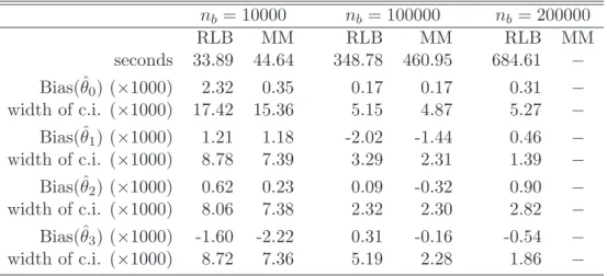
Table 2 shows the computation times in seconds, the bias of an MM-estimator computed for the whole data set and of the RLB estimator for B = 17, and the width of the com-ponentwise distribution-free confidence intervals based on the median at the 95%-level for different sub-sample sizes nb. The MM-estimates were computed with the function rlm
from the R-library MASS (Venables and Ripley, 2002). This function first computes an S-estimate as a starting point which has an approximate finite sample breakdown point of 0.5. Then an M-estimator with Tukey’s biweight and fixed scale is iteratively computed using this starting value that will inherit this breakdown point from the S-estimator. The time-consuming phase of MM-estimators is the computation of the highly robust starting value. The confidence intervals for the original MM-estimator were computed due to the asymptotical normality assumption. The distribution-free confidence intervals for the RLB estimator were based on the 5th and the 13th order statistics. Because the bias terms and
the width of the confidence intervals are very small due to the large sample size, the values in Table 2 are multiplied by 103.
In the considered situations RLB gave good results: the bias values are small, which shows that the RLB method indeed gave robust estimates, and the width of the confidence
nb = 10000 nb= 100000 nb= 200000 RLB MM RLB MM RLB MM seconds 33.89 44.64 348.78 460.95 684.61 − Bias(ˆθ0) (×1000) 2.32 0.35 0.17 0.17 0.31 − width of c.i. (×1000) 17.42 15.36 5.15 4.87 5.27 − Bias(ˆθ1) (×1000) 1.21 1.18 -2.02 -1.44 0.46 − width of c.i. (×1000) 8.78 7.39 3.29 2.31 1.39 − Bias(ˆθ2) (×1000) 0.62 0.23 0.09 -0.32 0.90 − width of c.i. (×1000) 8.06 7.38 2.32 2.30 2.82 − Bias(ˆθ3) (×1000) -1.60 -2.22 0.31 -0.16 -0.54 − width of c.i. (×1000) 8.72 7.36 5.19 2.28 1.86 −
Table 2: Results for robust linear regression with MM-estimator and RLB withB = 17. The computation of the MM-estimates for the whole data set withn= 17·200000 = 3.4·106 data points was not possible due to memory problems.
intervals is of similar size than for the original MM-estimator. It is not surprising that the distribution-free confidence intervals for the RLB estimator are somewhat larger (often by a factor between 1.1 and 1.2) than the confidence intervals of the MM-estimator based on the assumption of asymptotic normality. If the total sample size n is not too big, such that the MM-estimates can be computed with rlm only using the RAM of the computer, RLB only saves a little bit of computation time. However, one can fit much larger data sets using RLB for which the algorithm used byrlmwould need much more RAM than the available PC has (2 GB), such that the computation of the MM-estimates for the whole data set was impossible. In contrast to that, the computation time of RLB increased only approximately linearly in nb, and the used RAM was low in contrast to the used RAM to compute the MM-estimates for the whole data set. No memory problems occurred for RLB withn= 3.4·106 andB = 17.
Now we apply the RLB approach to kernel logistic regression (KLR), see (Wahba, 1999). KLR is a flexible method for classification problems and provides also estimates for the conditional probabilities P(Y = 1|X=x), x∈ X, which is not true for the support vector machine, see Bartlett and Tewari (2004). Christmann and Steinwart (2004) showed KLR has good robustness properties, e.g. a bounded influence function. All computations are done with the program myKLR (R¨uping, 2003) which is an implementation in C++ of the algorithm proposed by Keerthiet al.(2004) to solve the dual problem. We choose KLR for two reasons. Firstly, the computation of KLR needs much more time than for the support vector machine because the latter solves a quadratic instead of a convex program in dual space. Therefore, the need for computational improvements is greater for KLR than say for the SVM, and the potential gains of RLB can be more important. Secondly, the number of support vectors of KLR is approximately equal tonwhich slows down the computation of predictions.
sample size CPU time used cache available cache n in MB in MB 2000 4 sec 33 200 5000 25 sec 198 200 10000 5 min, 21 sec 200 200 10000 1 min, 33 sec 787 1000 20000 24 min, 11 sec 1000 1000 20000 14 min, 35 sec 1000 1000 100000 9 h, 56 min, 46 sec 1000 1000
Table 3: Computation times for kernel logistic regression using myKLR.
The simulated data sets contain ndata points (xi, yi)∈R8× {−1,+1} simulated in the
following way. All 8 components ofxi= (xi,1, . . . , xi,8) are simulated independently from a
uniform distribution on (0,1). The responsesyi are simulated independently from a logistic regression model according to P(Yi = +1|Xi =xi) = 1/(1 + exp[−f(xi)]). We define
f(xi) =
8 X
j=1
xi,j−xi,1xi,2−xi,2xi,3−xi,4xi,5−xi,1xi,6xi,7,
such that there are 8 main effects and 4 interaction terms. The data points are saved as ASCII files where xi,j is stored with four decimal places. The numerical results of fitting
kernel logistic regression to such data sets is given in Table 3. It is obvious that in this situation RLB can save a lot of computation time. If the whole data set has n = 105
observations, approximately 10 hours were needed to compute KLR. If RLB with B = 10 bits are used each with a sub-sample size of nb = 104, one needs approximately 10×93.3
seconds, i.e. 16 minutes, 1 GB of kernel cache available. This is a reduction by a factor of 38. If there are 5 CPUs available and each processor can use up to 200 MB kernel cache, RLB with B = 10 will need approximately 11 minutes which is a reduction by a factor of 55.
Christmann (2005) describes a strategy combiningε-support vector regression and kernel logistic regression to construct insurance tariffs. The whole data from 15 German motor vehicle insurance companies contains data from around 4.6 million customers with dozens of explanatory variables. A direct use of kernel logistic regression withmyKLR is unfeasable due to the computation time, see Table 3. Although a strategy was used to reduce the computational effort by exploiting certain characteristic features of such data sets, RLB offers an additional substantial reduction of the computation time. Fitting the model to the whole data set would need more than six months on a PC with 2.8 GHz CPU, whereas RLB with B = 17 using 2 CPUs was able to provide a good fit within 4 days: this is a reduction by a factor of 45. If RLB is allowed to use 8 CPUs the computation can be done in approximately one day and the reduction factor is around 180.
Concluding, RLB proved to be quite useful for kernel logistic regression for large data sets.
5. Discussion
In this paper robust learning from bites (RLB) was proposed to broaden the usability of computer-intensive robust estimators in the case of large data sets which occur nowadays often in data mining projects. RLB is especially designed for situations under which the original robust method cannot be used due to excessive computation time or due to memory space problems. In these situations RLB offers robust estimates and additionally robust confidence intervals. RLB estimators will in general not fulfill certain optimality criteria, but the method has four nice properties. Scalability: the number B of bites can be chosen such that the algorithm used to fit the bites needs less memory than the computer offers.
Performance: the computational steps for different bites can easily be distributed on several processors because they are independent and use disjoint parts of the data set. Robustness:
we considered the finite sample breakdown point and the influence function. These proper-ties are inherited from the original robust estimator computed for each bite and from the location estimator used to aggregate the results from the bites. Confidence intervals: no complex formulae are needed to obtain distribution-free (componentwise) confidence inter-vals for the estimates or for the predictions if the median is used in the aggregation step because the estimators computed from the B bites are independent and identically dis-tributed. Such confidence intervals for the predictions are especially interesting for general SVM methods (e.g. support vector machines and kernel logistic regression), because such methods have nice properties but finite sample confidence intervals for the predictions based on applying such methods once for the whole data set are typically unknown.
The subsampling approach used by RLB has connections to the remedian proposed by Rousseeuw and Bassett (1990) for univariate location estimation. The remedian with base
B computes medians of groups of nb observations, and then the medians of these medians
etc., until only a single estimate remains. The remedian needs onlyO(log(n)) total storage for fixed B which makes it especially useful for robust estimation in large data bases, for real-time engineering applications in which the data are not present at the same time and perhaps not stored, and for resistant aggregation of curves. RLB has also similarities to Rvote proposed by Breiman (1999) and DRvote with classification trees using majority voting proposed by Chawlaet al.(2004). Bootstrapping computer-intensive robust methods for huge data sets is often impossible due to computation time and memory limitations of the computer. The focus of the present paper was on robustness aspects and the computation of robust distribution-free confidence intervals for the median of the predictions even for very large data sets. Such confidence intervals are often a problem for robust estimators and general SVM methods based on Vapnik’s convex risk minimization principle. These topics were not covered in the papers mentioned above. RLB has also some similarity to the algorithms FAST-LTS and FAST-MCD developed by Rousseeuw and Driessen (1999, 2000) for robust estimation in linear regression or multivariate location and scatter models for large data sets. FAST-LTS and FAST-MCD split the data set into sub-samples, optimize the objective function in each sub-sample, and use these solutions as starting values to optimize the objective function for the whole data set. This is in contrast to RLB which aggregates estimation results from the bites to obtain robust confidence intervals.
Some good robust estimators are notn−1/2-consistent having a complicated non-normal
Davies (1990), Kim and Pollard (1990), Rousseeuw and Hubert (1999), Bai and He (1999), Aelstet al.(2002), Crouxet al.(2003), and Zuo and Cui (2005). Then RLB can be useful if distribution-free confidence intervals for the median of the predictions are needed for large data sets.
Acknowledgments
We thank Claudio Agostinello and Matias Salibian-Barrera for helpful discussions during ICORS-2005. The financial support of the Deutsche Forschungsgemeinschaft (SFB 475, ”Reduction of complexity in multivariate data structures”) and of the Forschungsband Do-MuS (University of Dortmund) is gratefully acknowledged.
Appendix
The appendix contains the proofs for the results given in Section 3.
Proof of Proposition 2. Obvious. ¤
Proof of Proposition 3. Obvious. ¤
Proof of Proposition 4. (i) follows from the linearity of the expectation operator. (ii) and (iii) follow from Slutzky’s theorem. ¤
Proof of Proposition 5. By construction of RLB the bites are disjoint and the estima-tors from the bites are independent. Assume that the original estimatorTS is consistent in
probability for TP. Then we have for allε >0 that
P (|medianb=1,...,BTSb(x)−TP(x)|< ε) ≥ P (|TSb(x)−TP(x)|< εfor all b= 1, . . . , B) = B Y b=1 P (|TSb(x)−TP(x)|< ε)→1, n→ ∞, x∈ X,
becauseB is fixed and limn→∞ (n/nb) =B. Now, assume that the original estimatorTS is
strongly consistent toTP. Then we obtain analogously
P ³ lim n→∞medianb=1,...,BTSb(x) =TP(x) ´ ≥ B Y b=1 P µ lim nb→∞ TSb(x) =TP(x) ¶ = 1, x∈ X,
because B is fixed and limn→∞ (n/nb) =B. ¤
Proof of Theorem 6. By assumption each biteSbis fitted with a general SVM estimator
having the representation
fSb,λnb(x) =
nb X
i=1
Because the bitesSb,b= 1, . . . , B, are disjoint, the RLB estimator of type I using a convex combination in the aggregation step is given by
fSRLB,B,(λ nb)(x) = B X b=1 cb nb X i=1 αi,bk(x, xi) (23) = n X i=1 B X b=1 cbαi,bk(x, xi), x∈ X. (24)
The formula (10) follows immediately. ¤
Proof of Proposition 8. (i) This follows immediately from (10).
(ii) Steinwart (2003, Th.9) proved that the general SVM estimator evaluated for the whole data set S has the property
Pr∗n(S ∈(X × Y)n; #SV(fS,λn)≥(SL,P−ε)n)→1, n→ ∞, (25)
if the conditions of the proposition are satisfied. Denote the outer probability measure of the product measure Pb,nb by Pr∗b,nb. The pairs (X
i, Yi) in the bites Sb,b = 1, . . . , B, are
independent and identically distributed by construction of RLB. Using (25) and n ≡Bnb
we obtain Pr∗n ³ S= (S1, . . . ,SB)∈(X × Y)n; #SV(fSRLB,B,(λnb))≥(SL,P−ε)n ´ (26) = Pr∗n à S = (S1, . . . ,SB)∈(X × Y)n; #SV(fSb,λnb)≥ B X b=1 (SL,P−ε)nb ! (27) ≥ Pr∗n ³ for all Sb ∈(X × Y)nb, b= 1, . . . , B; #SV(fSb,λnb)≥(SL,P−ε)nb ´ (28) = B Y b=1 Pr∗b,nb ³ Sb∈(X × Y)nb; #SV(fSb,λnb)≥(SL,P−ε)nb ´ →1, n→ ∞, (29) because cb∈(0,1),b= 1, . . . , B,B is fixed, and nb→ ∞. ¤
Proof of Theorem 9. The RLB estimator fRLB
S,B,(λnb) of type I is a convex combination
of fSb,λnb,b= 1, . . . , B, becausecb ∈(0,1) and PBb=1cb= 1. Therefore,
0 ≤ Z L(Y, fSRLB,B,(λ nb)(X)dP− R ∗ L,P = Z L Ã Y, B X b=1 cbfSb,λnb(X) ! dP− R∗L,P ≤ Z XB b=1 cbL ³ Y, fSb,λnb(X) ´ dP− R∗L,P (30) = B X b=1 cb ·Z L ³ Y, fSb,λnb(X) ´ dP− R∗L,P ¸ −→P 0, (31)
if limn→∞min1≤b≤Bnb → ∞. Here we used the convexity ofLin (30), theL-risk consistency
of the original estimator in (31), and (14). ¤
Proof of Theorem 11. The minimum number of points needed to modify TSb in bite b such that there is breakdown is given by nb ·ε∗nb(TSb) + 1, b = 1, . . . , B. The RLB
estimator breaks down if at least Bε∗
B(ˆµ) + 1 of the estimators TS1, . . ., TSB break down.
This gives the assertion. ¤
Proof of Theorem 14. Let z = (x, y) ∈ X × Y and P be a probability distribution on (X × Y,B(X × Y)). By assumption the RLB estimator has the property (20), i.e.
TSRLB,B = PBb=1cbT(PSb), where PSb denotes the empirical distribution of bite Sb, b =
1, . . . , B. Further, the influence function IF(z;T,P) exists by assumption of the theorem. It follows IF(z;TBRLB,P) = lim ε↓0 TRLB B ¡ (1−ε)P +εδz ¢ −TRLB B (P) ε = lim ε↓0 PB b=1cbT ¡ (1−ε)P +εδz ¢ −PBb=1cbT(P) ε = B X b=1 cblim ε↓0 T¡(1−ε)P +εδz ¢ −T(P) ε = IF(z;T,P),
which gives the assertion. ¤
References
Aelst, S. V., Rousseeuw, P. J., Hubert, M., and Struyf, A. (2002). The deepest regression method. Journal of Multivariate Analysis,81, 138–166.
Bai, Z. D. and He, X. (1999). Asymptotic distributions of the maximal depth estimators for regression and multivariate location. Annals of Statistics,27, 1616–1637.
Bartlett, P. L. and Tewari, A. (2004). Sparseness versus estimating conditional probabilities: Some asymptotic results. In Proceedings of the 17th Annual Conference on Learning Theory, Vol. 3120, Lecture Notes in Computer Science, Vol. 3120, pages 564–578, New York. Springer.
Bartlett, P. L., Jordan, M. I., and McAuliffe, J. D. (2006). Convexity, classification, and risk bounds. Journal of the American Statistical Association, to appear. http://stat-www. ~berkeley.~edu/tech-reports/638.~pdf.
Breiman, L. (1999). Pasting bites together for prediction in large data sets. Machine Learning,36, 85–103.
Chawla, N. V., Hall, L. O., Bowyer, K. W., and Kegelmeyer, W. P. (2004). Learning ensembles for bites: a scalable and accurate approach. Journal of Machine Learning Reseach,5, 421–451.
Christmann, A. (2005). On a strategy to develop robust and simple tariffs from motor vehicle insurance data. Acta Mathematicae Applicatae Sinica (English Series, Springer),
21, 193–208.
Christmann, A. and Steinwart, I. (2004). On robust properties of convex risk minimization methods for pattern recognition. Journal of Machine Learning Research,5, 1007–1034. Christmann, A. and Steinwart, I. (2005). Consistency and robustness of kernel based
re-gression. University of Dortmund, SFB-475, TR-01/05. Submitted. .
Croux, C., Van Aelst, S., and Dehon, C. (2003). Bounded influence regression using high breakdown scatter matrices. Annals of the Institute of Statistical Mathematics,55, 265– 285.
David, H. A. and Nagaraja, H. N. (2003). Order Statistics, 3rd ed. . Wiley & Sons, New York.
Davies, P. L. (1990). The asymptotics of S-estimators in the linear regression model. Annals of Statistics,18, 1651–1675.
Davies, P. L. (1993). Aspects of robust linear regression.Annals of Statistics,21, 1843–1899. Devroye, L., Gy¨orfi, L., and Lugosi, G. (1997). A Probabilistic Theory of Pattern
Recogni-tion. Springer, New York.
Donoho, D. L. and Huber, P. J. (1983). The notion of breakdown point. In P. J. Bickel, K. A. Doksum, and J. L. Hodges, editors, A Festschrift for Erich L. Lehmann, pages 157–184. Jr. , Belmont, California, Wadsworth.
Hampel, F. R. (1968). Contributions to the theory of robust estimation. Ph. D. thesis, Dept. Statistics, Univ. California, Berkeley.
Hampel, F. R. (1974). The influence curve and its role in robust estimation. Journal of the American Statistical Association,69, 383–393.
Hampel, F. R., Ronchetti, E. M., Rousseeuw, P. J., and Stahel, W. A. (1986). Robust statistics: The Approach Based on Influence Functions. Wiley, New York.
Hand, D., Mannila, H., and Smyth, P. (2001). Principles of Data Mining. MIT Press, Cambridge, Massachusetts.
Hipp, J., G¨untzer, U., and Grimmer, U. (2001). Data quality mining - making a virtue of necessity. Workshop on Research Issues in Data Mining and Knowledge Discov-ery DMKD, Santa Barbara, CA, http://www.~cs.~cornell.~edu/johannes/papers/ dmkd2001-papers/p5_hipp.~p%df.
Keerthi, S. S., Duan, K., Shevade, S. K., and Poo, A. N. (2004). A fast dual algorithm for kernel logistic regression. In Machine Learning: Proceedings of the Ninetheenth Interna-tional Conference (Eds: C. Sammut, A. G. Hoffmann), pages 299–306. Kaufmann, San Francisco.
Kim, J. and Pollard, D. (1990). Cube root asymptotics. Annals of Statistics,18, 191–219. Le Cam, L. (1980). In: Discussion of ”minimum chi-square, not maximum likelihood!
Annals of Statistics,8, 473–478.
Rousseeuw, P. J. (1984). Least median of squares regression. Journal of the American Statistical Association,79, 871–880.
Rousseeuw, P. J. and Bassett, G. W. (1990). The remedian: a robust averaging method for large data sets. Journal of the American Statistical Association,85(409), 97–104. Rousseeuw, P. J. and Driessen, K. V. (1999). A fast algorithm for the minimum covariance
determinant estimator. Technometrics,41, 212–223.
Rousseeuw, P. J. and Driessen, K. V. (2000). An algorithm for positive-breakdown regression based on concentration steps. In O. O. W. Gaul and M. Schader, editors,Data Analysis: Scientific Modeling and Practical Application, pages 335–346, New York. Springer. Rousseeuw, P. J. and Hubert, M. (1999). Regression depth. Journal of the American
Statistical Association,94, 388–402.
R¨uping, S. (2003). myKLR - kernel logistic regression. University of Dortmund, Department of Computer Science, http://www-ai.~cs.~uni-dortmund.~de/SOFTWARE.
Sch¨olkopf, B. and Smola, A. J. (2002). Learning with Kernels. Support Vector Machines, Regularization, Optimization, and Beyond. MIT Press, Cambridge, Massachusetts. Steinwart, I. (2001). On the influence of the kernel on the consistency of support vector
machines. Journal of Machine Learning Research,2, 67–93.
Steinwart, I. (2002). Support vector machines are universally consistent. J. Complexity,
18, 768–791.
Steinwart, I. (2003). Sparseness of support vector machines. Journal of Machine Learning Research,4, 1071–1105.
Steinwart, I. (2005a). Consistency of support vector machines and other regularized kernel machines. IEEE Transactions on Information Theory,51, 128–142.
Steinwart, I. (2005b). How to compare loss functions and their risks. Technical report, Los Alamos National Laboratory. http://www.~c3.~lanl.~gov/~ingo/pubs.~shtml. Tsybakov, A. B. (2004). Optimal aggregation of classifiers in statistical learning. Annals of
Statistics,32, 135–166.
Vapnik, V. N. (1998). Statistical Learning Theory. Wiley, New York.
Venables, W. N. and Ripley, B. D. (2002). Modern Applied Statistics with S, 4thed. .
Wahba, G. (1999). Support vector machines, reproducing kernel hilbert spaces and the randomized gacv. In B. Sch¨olkopf, C. J. C. Burges, and A. J. Smola, editors, Advances in Kernel Methods - Support Vector Learning, pages 69–88, Cambridge, MA. MIT Press. Yohai, V. J. (1987). High breakdown-point and high efficiency robust estimates for
regres-sion. Annals of Statistics,15, 642–656.
Zhang, T. (2004). Statistical behaviour and consistency of classification methods based on convex risk minimization. Annals of Statistics,32, 56–134.
Zuo, Y. and Cui, H. (2005). Depth weighted scatter estimators. Annals of Statistics,33(1), 381–413.
Andreas Christmann Ingo Steinwart University of Dortmund CCS-3
Department of Statistics Mail Stop B256
44221 Dortmund Los Alamos National Laboratory GERMANY Los Alamos, NM 87545
E-mail: USA
[email protected] E-mail: [email protected]
Mia Hubert
Department of Mathematics Katholieke Universiteit Leuven W. de Croylaan 54
B-3001 Leuven BELGIUM