Faculty of Science and Technology MASTER S THESIS. Title of thesis: Low-frequency reflection seismic and direct hydrocarbon indication.

(1)

Faculty of Science and Technology

MASTER’S THESIS

Study program/Specialization: Petroleum Geosciences Engineering

Spring, 2014 Open Writer:

Xiaoan Zhong

(Writer’s signature) Faculty supervisor: R. James Brown

External supervisor(s): Børge Rosland Title of thesis:

Low-frequency reflection seismic and direct hydrocarbon indication Credits (ECTS): 30 Keywords: Low frequency Amplitude attenuation Hydrocarbon indication Reflection seismic Spectral decomposition

Instantaneous spectral analysis

Pages: 65 Stavanger, 15th_{June, 2014} Copyright by Xiaoan Zhong 2014

(2)

(3)

Low-frequency reflection seismic and direct hydrocarbon indication

by

Xiaoan Zhong, B.Sc.

Thesis

Presented to the Faculty of Science and Technology The University of Stavanger

The University of Stavanger

June 2014

(4)

(5)

Acknowledgements

This thesis report is submitted in partial fulfillment of the requirements for the Master of Science degree in Petroleum Geosciences Engineering. The research has mainly been carried out at the offices of Skagen44 AS in Stavanger, Norway.

The author would like to acknowledge Skagen44 AS for providing all of the seismic, well and scientific data used within this study. Special thanks are given to Børge Rosland as the external supervisor for this study. Thanks to Oskar Fjeld and Olav Høiland for assisting with the regional tectonic history and stratigraphic correlation.

The author would like to express his gratitude to Professor R. James Brown for guidance through this project and providing idea-motivation to accomplish this study.

Finally, the author would like to thank the department of Petroleum Geosciences for awarding the COREC (Center for Oil Recovery) Scholarship during his two-year study in the University of Stavanger.

(6)

(7)

Abstract

Low-frequency reflection seismic and direct hydrocarbon indication

Xiaoan Zhong, M.Sc. The University of Stavanger, 2014

Supervisors: R. James Brown; Børge Rosland

Low-frequency reflection seismic has been used as an indicator to detect hydrocarbons in petroliferous reservoirs. A number of spectral decomposition methods have been developed to derive seismic from time to frequency domain. The application of low-frequency seismic computed by the Gabor-Morlet transform (GMT) and instantaneous spectral analysis (ISA) methods revealed one of low-frequency shadow effects, amplitude attenuation, in the southern North Sea. According to computed low-frequency (< 20 Hz) instantaneous spectral profiles through discovered wells, strong responses are observed on hydrocarbon-saturated intervals. By contrast, on higher frequency (> 20 Hz) instantaneous spectral profiles, frequency amplitude is vanished from the petroliferous intervals, however, strong responses are presented either above or below these pay zones. The loss mechanism of high-frequency energy is considered to be contributed by P-wave attenuation of stratigraphic heterogeneity. This type of low-frequency shadow effect can illustrate the probable existence of an oil reservoir and can be applied to detect the existence of hydrocarbon directly. Based on the distribution of attenuated frequency amplitude, a total of 140 km2_{of prospects have been identified from both Cretaceous-Paleogene} chalk reservoirs and sandstones beneath the basal Cretaceous unconformity (BCU).

(8)

The identified chalk prospects are mainly distributed along the rim of anticlines on the Lindesnes Ridge, while prospective clastics are stratigraphically entrapped on the slope of the Grensen Nose. In addition to using low-frequency reflection seismic to detect hydrocarbon directly, frequency components can be applied to calibrate the interpretations of horizons and faults as well.

(9)

List of Figures

Figure 1. Instantaneous spectral sections corresponding to the stacked seismic

profile ...2

Figure 2. ISA sections corresponding to the stacked seismic profile ...4

Figure 3. Location map of study area in the southern North Sea ...5

Figure 4. Stratigraphic chart of southern North Sea ...6

Figure 5. Top Eldfisk field structural map ...9

Figure 6. 3D reflection seismic coverage map ...10

Figure 7. PSTM gather computation ...11

Figure 8. 2D seismic time structural map of BCU...13

Figure 9. 2D seismic time structural map of Top Cretaceous ...15

Figure 10. 2D seismic time structural map of Top Paleogene ...17

Figure 11. Synthetic profile of 2/7-31 well ...18

Figure 12. Seismic and geological sections through 2/7-19, 2/7-22, and 2/11-2 wells ...19

Figure 13. Depth-structure contour map of the BCU ...21

Figure 14. Depth-structure contour map of the base of Cretaceous chalk ...22

Figure 15. Depth-structure contour map of Top Cretaceous ...23

Figure 16. Depth-structure contour map of Top Balder Formation, Paleocene ...24

Figure 17. Depth-structure contour map of Top Shetland Group, Paleogene ...25

Figure 18. ISA gather with frequencies from 2Hz to 15 Hz at the well location ..28

Figure 19. Seismic lines for spectral sections through key wells ...31

Figure 20. XL2650 spectral sections corresponding to the stacked seismic profile ...32

(12)

Figure 22. XL2840 spectral sections corresponding to the stacked seismic profile

...34

Figure 25. IL2112 spectral sections corresponding to the stacked seismic profile37 Figure 26. Low-frequency attribute within 200ms below BCU ...40

Figure 27. Medium-frequency attribute within 200ms below BCU ...41

Figure 28. High-frequency attribute within 200ms below BCU...42

Figure 29. BCU structural map overlying low-frequency anomalies ...43

Figure 30. Low-frequency attribute within 200ms below Top Cretaceous ...44

Figure 31. Medium-frequency attribute within 200ms below Top Cretaceous ...45

Figure 32. High-frequency attribute within 200ms below Top Cretaceous ...46

Figure 33. Top Cretaceous structural map overlying low-frequency anomalies ...47

Figure 34. Low-frequency attribute within 180ms below Top Paleogene ...48

Figure 35. Medium-frequency attribute within 180ms below Top Paleogene ...49

Figure 36. High-frequency attribute within 180ms below Top Paleogene ...50

Figure 37. Top Paleogene structural map overlying low-frequency anomalies ....51

Figure 38. BCU clastic-reservoir polygons from low-frequency attribute slice ....52

Figure 39. 10 Hz spectral section corresponding to the stacked seismic profile ...53

Figure 40. 8 Hz spectral section corresponding to the stacked seismic profile ...54

Figure 41. 7.2 Hz spectral section corresponding to the stacked seismic profile ..55

Figure 42. Cretaceous chalk reservoirs prospects from low-frequency seismic ....56

(13)

List of Tables

Table 1. ISA volume list through key wells ...11

(14)

(15)

1 Introduction

As a significant part of reflected seismic waves, anomalous frequencies less than 20 Hz appear to have been first observed to be associated with hydrocarbon reservoirs by Taner et al. (1979). Since then, a number of laboratory and field examples have been reported in the literature where the low-frequency components of reflected seismic waves have been used as hydrocarbon indicators to image, delineate, and monitor petroliferous reservoirs (Taylor et al., 2000; Cai et al., 2008; Wang et al., 2009; Liu et al., 2010; Pu, 2011; Long et al., 2012; Yang et al., 2012). These indicators include low-frequency shadow with hydrocarbon deposits, low-frequency energy anomalies, and instantaneous wavelet energy absorption analysis, etc. (Chen et al., 2012).

In reflection-seismic field data acquired for petroleum exploration and/or production, low-frequency shadow effects, such as time delay, phase distortion, frequency decrease, and amplitude attenuation, have been observed and provided evidences of hydrocarbon existence (Goloshubin et al., 2002; Castagna et al., 2003; Sinha et al., 2005; Odebeatu et al., 2006; Huang et al., 2007; Kazemeini et al., 2009; Silin et al., 2010; Yu et al., 2011; Zhang et al., 2012; Chen et al., 2013).

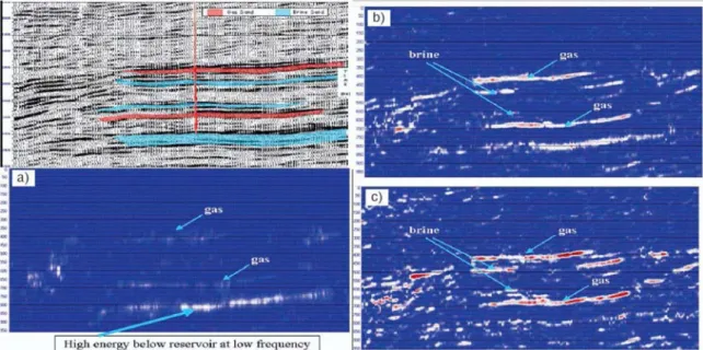
For example, Chen et al. (2012) computed a series of instantaneous spectral sections from stacked seismic data (Figure 1a), and illustrated amplitude attenuation effect by comparing produced spectral profiles. On the 12 Hz section (Figure 1b), the bright gas reservoir (indicated by a black arrow) and strong low-frequency shadow (outlined by a black contour) lie immediately underneath the reservoir. On the 36 Hz section (Figure 1c), the gas reservoir still remains bright, whereas the low-frequency shadow has disappeared.

(16)

Figure 1. Instantaneous spectral sections corresponding to the stacked seismic profile

To derive frequency components from reflection seismic, spectral decomposition has been regarded as an effective technology. As summarized by Castagna et al. (2003), three steps are involved for spectral decomposition: (1) utilize wavelet transform methods to decompose the seismogram into constituent wavelets; (2) produce “frequency gathers” by summing up the transformed spectra (e.g. Fourier spectra) of the individual wavelets in the time-frequency domain; and (3) sort the frequency gathers to produce common frequency cubes, sections, time slices, and horizon slices, etc.

There are a variety of spectral decomposition methods, which include the discrete Fourier transform (DFT), the short-time Fourier transform (STFT), enhanced spectral processing (ESP), the maximum entropy method (MEM), the continuous wavelet transform (CWT), matching pursuit decomposition (MPD), the Gabor-Morlet transform (GMT), and instantaneous spectral analysis (ISA), etc.

Qian et al. (1994) and Partyka et al. (1999) applied the discrete Fourier transform (DFT) to generate discrete-frequency energy cubes for reservoir characterization. However, vertical resolution of the DFT is limited due to frequency localization loss when the seismogram is windowed (Castagna et al., 2003; Sinha et al., 2005).

The short-time Fourier transform (STFT) extracts the frequency content of the signal and produces a 2D representative profile of frequencies versus time by adding a small time-domain window and shifting this window appropriately (Okaya et al.,

(17)

1992). The vertical resolution is fixed over the entire time-frequency plane when a window function has been chosen for an STFT.

Enhanced spectral processing (ESP) eliminated the windowing problem in the above Fourier spectral analysis (Sun et al., 2002).

The continuous wavelet transform (CWT) decomposes a function by band-pass filtering the original signal at different band-widths. In practice, the CWT has higher frequency resolution for low frequencies and better time resolution for higher frequencies (Chakraborty et al., 1995). As an extensional version of CWT, Stockwell et al. (1996) introduced an S-transform algorithm based on a moving and scalable localizing Gaussian window. Differentiating itself from other methods, S-Transform is an invertible transform which is closely related to the Fourier transform.

Mallat et al. (1993) introduced the matching-pursuit decomposition (MPD) to detect low-frequency shadows beneath hydrocarbon reservoirs. Because of excellent localization behavior of the MPD, reflections can be enhanced and surface waves and other types of noise can be eliminated using polygonal filters (Chakraborty et al., 1995; Huang et al., 2007).

Castagna et al. (2003) presented a method known as instantaneous spectral analysis (ISA).The ISA method selects the wavelet dictionary to better capture the features of the seismogram while selecting parameters judiciously and avoiding as many cross-correlation operations as possible to achieve reasonable computation time. Testified by various field examples, spectral decomposition with ISA has been done accurately with acceptable speed while simultaneously achieving excellent time and frequency resolution. As one of their examples, low-frequency shadow beneath the gas-filled sandstone reservoirs (red filled on stacked seismic) shows strongest event on the 10 Hz common-frequency section (Figure 2a), then it persists but is weaker than the overlying gas sands on the 20 Hz common-frequency section (Figure 2b), and finally it has disappeared on the 30 Hz common-frequency section (Figure 2c).

(18)

Figure 2. ISA sections corresponding to the stacked seismic profile

The Gabor-Morlet transform (GMT) filters the seismic data with a series of Gabor-Morlet wavelets to obtain narrow-band analytic traces. Divided by the original trace envelope, narrow-band traces are normalized to remove the amplitude variation of individual reflected events (Morlet et al., 1982, Taner 1983, Qian et al., 1999).

All spectral decomposition methods have their own advantages and disadvantages, different methods are required regarding to different applications (Castagna et al., 2006; Pang et al., 2013).

In this project, the ISA method is applied to generate frequency spectra along specific seismic lines, and the computed frequency spectra range from 2 to 15 Hz at steps of 1 Hz. The purpose of creating ISA volumes is to match frequency responses with fluid content which was reported by penetrated wells.

In the Rock Solid Attribute module of IHS Kingdom software, the GMT method is applied to produce time-frequency envelopes of user-defined frequency bands. Frequency attribute analysis is performed on these envelopes to identify low-frequency shadow effects.

(19)

2 Geological background

The study area is located in the Western Graben of the southern North Sea, approximately 260 km southwest of the Farsund coast, Norway, and it is adjacent to the United Kingdom and Denmark sectors (Figure 3). As a proved petroliferous province, several oil and gas fields have been discovered on Lindesnes Ridge, e.g. Eldfisk, Embla, Valhall, and Hod, etc. (Figure 4). This research is focused on the depression between the Grensen Nose and the Lindesnes Ridge, which is bounded by several prominent NW-SE normal faults (Zanella et al., 2003; Gennaro et al., 2013).

Figure 3. Location map of study area in the southern North Sea

(Tectonic framework after Brekke, 2000; location map after Gennaro et al., 2013)

GYDA ULA VALHALL EKOFISK TOR BLANE OSELVAR ALBUSKJELL HOD ELDFISK EDDA EMBLA COD GYDA TAMBAR MIME ELDFISK VEST EKOFISK HOD TRYM TAMBAR ØST TOMMELITEN GAMMA 450000.000000 450000.000000 470000.000000 470000.000000 490000.000000 490000.000000 510000.000000 510000.000000 530000.000000 530000.000000 550000.000000 550000.000000 570000.000000 570000.000000 590000.000000 590000.000000 61 90 00 0 .0 0 000 0 61 90 00 0 .0 0 000 0 62 10 00 0 .0 00 00 0 62 10 00 0 .0 00 00 0 62 30 00 0 .0 00 00 0 62 30 00 0 .0 00 00 0 62 50 00 0 .0 00 00 0 62 50 00 0 .0 00 00 0 62 70 00 0 .0 0 00 00 62 70 00 0 .0 0 00 00 62 90 00 0 .0 00 00 0 62 90 00 0 .0 00 00 0 63 10 00 0 .0 00 00 0 63 10 00 0 .0 00 00 0 63 30 00 0 .0 00 00 0 63 30 00 0 .0 00 00 0 0 5 10 20 30 40 km ) ) ) ) )) )) )) )) )) )) Oil fields Gas fields Discoveries Area of interest U K s_e c t o_r U K s e c t o r N or w a y s e ct o r N or w a y s e ct o r D en m a rk s ec t o r D en m a rk s ec t o r Fe da_G rab en Coffe_{e So} il Fa_ult Søg ne B asin M an_da l h igh Grensen Nose Lind es nes R idg_e Jos_eph ine Hig_h Hidr_{al h} igh Weste_{rn Gra} ben

(20)

Figure 4. Stratigraphic chart of southern North Sea

(References of the chart are listed on the right-hand side of the column)

Lithostratigraphy Hydrocarbon fields & wells Tectonic events Age (Ma) 2.6 66 145 201 252 299 Notes:

[1] Numerical ages, systems, and series are referenced from International Chronostratigraphic Chart v2013/01. International Commission on Stratigraphy. [2] Lithostratigrapgy chart after Permian is modified from Deegan et al. (1977), Rossland et al. (2013), and Brasher et al. (1996).

[3] Lithostratigrapgic chart of Carboniferous is modified from Casey et al. (1993). [4] Lithostratigrapgy chart of Devonian is modified from Lee et al. (1993).

[5] Tectonic events are

summarized after Blystad et al .

(1995) & Zanella et al. (2003).,

[6] Hydrocarbon fields and wells are based on Factpages of Norwegian Petroleum Directorate public database.

Legends End Jurassic

compression

North Sea dome uplift &

erosion First episode of rifting ? Sandtone Silty claystone 359 419 Coal Carbonate Evaporite Conglomerate N ORD LAND GRO UP

E KOFIS K FM TOR FM H OD FM C ROME R KNO LL U LA FM U LA FM MAND AL FM FA RS UN D FM B RYN E FM S MITH B ANK FM Z E CHS TE IN ROTLIE GE ND ES 2/11-2Hod Embla 2/7-2 Hod 2/7-31 2/7-19 2/7-29 Embla 2/7-31 2/10-1S 2/7-22 Gas shows Oil shows Oil Second episode of rifting Third episode of rifting Sag phase ? Fourth episode of rifting and onset of sea-floor spreading Onset of sea-floor spreading and renewed rifting Localized inversion Chronostratigraphy Te rt ia ry C ret ac eo u s T ri a ss ic J u ra ss ic Pe rm ia n Ne o g en e Pa le og e n e Upp e r Lo w e r Lopingian Up p e r Lo w e r M id d le Quaternary Miocene Pliocene Paleocene Eocene Oligocene Campanian Maastrichtian Turonian Coniacian Santonian Cenomanian Aptian Albian Valanginian Hauterivian Barremian Berriasian Bajocian Bathonian Callovian Aalenian Oxfordian Kimmeridgian Tithonian Carnian Norian Rhaetian Sinemurian Pliensbachian Toarcian Hettangian Olenekian Anisian Ladinian Induan Up pe r Lo w e r M id dl e Guadalupian Cisuralian Ca rb on if e rou s Pennsylvanian Mississippian De v o ni a n Up p e r Lo w e r M id d le Famennian Frasnian Givetian Eifelian Lochkovian Pragian Emsian

H ORD ALAN D GR OUP B ALDE R FM

(21)

2.1 Tectonic events

According to Müller et al. (1992), Brekke (2000), Mosar (2003), Zanella et al. (2003), Wilson et al. (2006), Gołedowski et al.(2012), and Rossland et al. (2013), the southern North Sea underwent eight stages of tectonic events: (1) sag phase during Devonian; (2) first extension and rifting episode from Carboniferous to Permian; (3) second extension and rifting episode during Triassic; (4) North Sea dome rift and erosion in early Jurassic; (5) third extension and rifting episode during middle to late Jurassic; (6) end Jurassic compression; (7) fourth rifting episode and onset of sea-floor spreading during early Cretaceous; (8) onset of sea-sea-floor spreading and renewed rifting from late Cretaceous to early Paleogene; and (9) localized inversion in Neogene (Figure 4).

There is a significant tectonic and sedimentary break between Late Jurassic and Early Cretaceous. The contact surface of the strata is featured by a widely distributed unconformity throughout the North Sea, which is called “basal Cretaceous unconformity” or “BCU” for abbreviation (Rawson et al., 1982; Blystad et al., 1995).

2.2 Petroleum systems and entrapment

Discovered fields have proved a working petroleum system in southern North Sea, especially on the Lindesnes Ridge. Based on trapping mechanism, there are two types of entrapment: (1) Pre-Cretaceous structural and stratigraphic trap with dip and fault closure laterally and overburden shale sealing vertically, e.g. Embla Field, the 2/7-19 discovery, and the 2/7-31 discovery, etc. (Marshall et al., 2003; NPD, 2014); and (2) Late Cretaceous to Paleocene fractured anticline overlying steeply dipping salt structures, e.g. Eldfisk Field, Valhall Field, Hod Field, etc. (Surlyk et al., 2003; NPD, 2014).

(22)

2.2.1 Embla Field

Located on the western flank of Lindesnes Ridge, the Embla field was discovered in 1974 by the 2/7-9 well, and it has Pre-Jurassic structural and stratigraphic trapping with dip and fault closure laterally and Jurassic shale sealing vertically (Marshall et al., 2003). Reservoir rocks comprise over 400 m of braided fluvial and alluvial fan sandstones from Devonian to Permian, and are interbeded by a complex floodplain/lacustrine mudstone, volcanic, and intrusive unit (Knight et al., 1993; Munz et al., 1998).

Ohm et al. (2012) performed geochemistry analysis and suggested that oil of Paleozoic age charged the field at the end of the Triassic. The Paleozoic oil was biodegraded at the oil-water contact during the Jurassic uplift and erosion, which caused poor production on the flank. Meanwhile, hydrocarbons in the crest of the structure escaped due to erosion of the seal. Subsidence occurred during the Cretaceous and formed a new seal and the Upper Jurassic oil reached a mature window and charged the structure along its carrier system.

2.2.2 Eldfisk Field

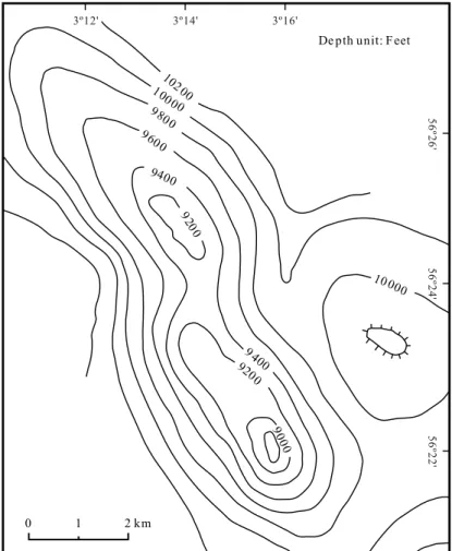
Located in the northern part of Lindesnes Ridge, the Eldfisk field was discovered in 1970 with the 2/7-1X well, and is one of the largest chalk fields with four-way closure (Herrington et al., 1991). Salt diapirism from the Upper Permian Zechstein Group penetrated through the overlying beds and generated significant anticlines in shallower formations (Jenyon 1985). The Eldfisk structure comprises three domes which were induced by salt flowage (Figure 5).

The Eldfisk reservoirs are composed of chalks of the Paleocene Ekofisk Formation, and the Late Cretaceous Hod and Tor Formations (Brasher et al., 1996).

In the Eldfisk field, hydrocarbons were generated from Upper Jurassic Kimmeridgian shale charged into chalk reservoirs and then effectively sealed by fine-grained Paleogene mudstone (Gautier 2005).

(23)

Figure 5. Top Eldfisk field structural map (Modified after Maliva et al., 1992)

102₀₀ 100₀₀ 980₀ 960₀ 9400 92₀₀ 9 40₀ 920₀ 90 00 1000₀ 0 1 2 km 3º12' 3º14' 3º16' 56 º2 6' 56 º2 4' 56 º2 2' De pth unit: F eet

(24)

3 Database

From this chapter on, all figures and tables were produced by the author.

3.1 Seismic data

The research area is covered by a 1585 km2_{of 3D reflection seismic survey} acquired in 2012. This is a modern broadband data set with record length of 7680 ms. The acquisition sampling rate was 2 ms and the processing was performed at 4 ms sampling. However, seismic volumes of dataset are limited within a 554 km2_coverage (Figure 6).

Figure 6. 3D reflection seismic coverage map

4100 3900 3700 3500 3300 3100 2900 2700 2500 2300 2100 1900 1700 1500 1300 1100 900 700 600 4100 3900 3700 3500 3300 3100 2900 2700 2500 2300 2100 1900 1700 1500 1300 1100 900 700 600 19 00 21₀₀ 23 00 25 00 27₀₀ 29 00 31 00 33₀₀ 35 00 37 00 39₀₀ 41 00 43 00 45₀₀ 19 00 21 00 23₀₀ 25 00 27 00 29 00 31 00 33 00 35 00 37 00 39 00 41 00 43 00 45 00 0 2 4 6 8 10 km 500000 510000 520000 530000 540000 490000 6 25 00 00 62 6 00 00 62 40 00 0 62 30 00 0 62 20 0 00 62 1 00 0 0 500000 510000 520000 530000 540000 490000 6 25 00 00 62 6 00 00 62 40 00 0 62 30 00 0 62 20 0 00 62 1 00 0 0 2/10-2 _Wells Inline Crossline 3D volume North 2/7-9 2/7-19 2/7-31 2/7-29 2/7-22 2/7-2 2/10-2 2/10-1S 2/11-8 2/11-9 2/11-5 2/11-2 A B

(25)

Available seismic volumes consist of the following groups: (1) a post-stack time migration (PSTM) gather under positive polarity; (2) full-volume time-frequency envelopes of 4.8, 7.2, 9.4, 12, 15.5, 20, 30, 40, and 50 Hz common frequencies; and (3) 2 to 15 Hz ISA cubes crossing key wells at steps of 1 Hz (Table 1).

Table 1. ISA volume list through key wells

No. Well Direction

Inline Crossline 1 2/7-2 2522 2 2/7-9 3208 3 2/7-19 2688 3306 4 2/7-22 2700 5 2/7-29 2466 3176 6 2/7-31 2618 7 2/10-1S 2410 8 2/10-2 2112 9 2/11-2 3190 10 2/11-5 3156 11 2/11-8 2648 12 2/11-9 3144

A tuning-thickness analysis was performed to determine the vertical resolution for this survey, the author suggests that the minimum resolvable time-thickness of a bed is 9 ms (Figure 7a).

Figure 7. PSTM gather computation

(a) Tuning thickness analysis; (b) computed spectrum; (c) computed wavelet. (Computations are done by the author)

0

Apparent time thickness (sec)

0.01 0.02 0.03 0.04 0.05 0.06 A ct u a l t im e th ic k n es s (s ec) 0.00 0.01 0.02 0.03 0.04 0.05 0.060.0 0.5 1.0 1.5 2.0

Normalized peak-trough amplitude

0 25 50 75 Frequency (Hz) 0.0 0 5. 1.0 100 Si gnal s pe ctrum N ois e spectrum -1.0 -0.1 0 Time (Second) -0.2 0.1 0.2 1.0 -0.5 0 0.5 1

(26)

In addition, the computed spectrum of PSTM gathers (Figure 7b) indicates that the frequency of seismic volume has higher concentration between 5 and 20 Hz, which is thought to be favorable frequency band for determining fluid mobility.

Moreover, a zero-phase wavelet for the PSTM gather was computed for further synthetics processing (Figure 7c).

Nevertheless, due to the influence of gas in reservoirs, 3D seismic data from the Lindesnes Ridge is obscure and of poor quality. As a solution, more than 1600 km of 2D seismic data were interpreted to demonstrate the structures along key horizons in the Western Graben.

3.2 Hydrocarbon discoveries from NPD wells

In the area of interest, 12 exploration wells have been penetrated since 1970, most of which were reported with hydrocarbons (NPD, 2014). Well data was extracted and summarized from the shared database of the Norwegian Petroleum Directorate (NPD).

3.2.1 Hydrocarbon beneath BCU

Oil and gas were proved beneath BCU during drill stem tests (DST) or core analysis from the 2/7-9, 2/7-19, 2/7-22, 2/7-29, and 2/7-31 wells. Fluids from these wells show that hydrocarbon was found surrounding the rim of the northern sub-sag of the Western Graben source kitchen (Figure 8).

(1) 2/7-9 well

The Embla field was found due to discoveries in the 2/7-9 well, and its reservoirs comprise sands from Devonian to Permian. A 111-m net pay zone with average porosity of 13 % and oil saturation of 55 % was encountered in the Late Jurassic sands. One DST was performed in the Devonian sandstones at 4313-4356 m, showing that 36 sm3_{(standard cubic meters) oil and 10 000 sm}3_{gas per day was} produced through a 32/64" choke after acidation.

(27)

Gas-bearing sands were encountered in the Upper Jurassic Ula Formation, and hydrocarbon was proved in the re-entry DST due to a blow-out preventer (BOP) system problem in the original well. Acid-treated Upper Jurassic sands produced 34.8 sm3_{oil and 15 631 sm}3_{gas per day through an 11.91 mm choke.}

Figure 8. 2D seismic time structural map of BCU

(3) 2/7-22 well

A 14-m pay zone was interpreted from Devonian alluvial clean sands at 4435.5-4502.0 m interval, and the oil-water contact was predicted at 4502 m. One

(28)

DST test was performed at the 4489-4496 m interval and flowed 207 sm3_of condensate and 347 sm3_{of water per day through a 12.7 mm choke.}

(4) 2/7-29 well

Overall 160.5 m gross of sands were penetrated in the Upper Jurassic interval. A one-gallon dead-oil sample was obtained in the Eldifisk Formation sandstone. No DST was performed.

(5) 2/7-31 well

A DST was performed over the Upper Jurassic Ula Sandstone 4565.9-4623.8 m interval. The well flowed at an average stabilized rate of 283 sm3_{of oil and 120} 000 sm3_{of gas on a 16/64" choke.}

Wireline formation pressure tests were taken throughout the Permian Rotliegendes section. Oil samples were recovered from two FMT tests at 4793 m and 4812 m.

(6) 2/10-1S well

A gas kick appeared while drilling at 4343 m in the Permian Rotliegendes sand. A DST was planned to the Rotliegendes sand interval, but it was not carried out due to a leak in the casing.

3.2.2 Hydrocarbon in chalk reservoirs

Discoveries in Cretaceous to Paleocene chalk reservoirs were made in Eldfisk field, Valhall field, and Hod field. Hydrocarbons were tested by the 2/7-2, 2/7-31, and 2/11-2 wells, and oil shows were reported from the 2/7-9, 2/7-19, 2/11-5 and 2/11-9 wells (Figure 9).

(29)

Figure 9. 2D seismic time structural map of Top Cretaceous

(1) 2/7-2 well

Oil shows were observed on the 3013.9-3027.9 m cores in the Tor Formation. One DST was performed at 3005.3-3017.5 m interval of the uppermost Tor Formation. 6.83 m3_{load water and 0.68 sm}3_{oil was flowed. After acidization, 54.6} sm3_{of oil, 44.7 m}3_{of formation water, and 4814 sm}3_{of gas were produced.}

(2) 2/7-9 well

Good shows were recorded in the Paleocene Danian limestone and Cretaceous Chalk intervals. However, no hydrocarbons were tested from either reservoir.

(30)

(3) 2/7-19 well

Some fluorescence was observed in the Late Cretaceous chalk reservoirs. (4) 2/7-31 well

Hydrocarbon shows were recorded in the Lower Cretaceous Tuxen Formation. (5) 2/10-2 well

Weak shows were reported in the Late Cretaceous Tor Formation from cores and cutting samples.

(6) 2/11-2 well

Quality oil-bearing chalk reservoirs were encountered in the Late Cretaceous Hod Formation below 2640.5 m. A 51.5-m net pay was estimated with average porosity of 27.7 % and an average water saturation of 40.3 %. Two runs of DST were carried out in the Hod Formation, both tests produced oil and gas, no water. The maximum flow rate was achieved while testing the 2642.6-2665.5 m interval, with 546 sm3_{of oil and 82 120 sm}3_{of gas per day.}

(7) 2/11-5 well

Fair dull golden fluorescence and fair cut were reported in the Upper Jurassic chalk reservoirs. However, these sections were found below the oil-water contact and no moveable hydrocarbons were presented.

(8) 2/11-9 well

Oil shows associated with fractures were observed in the Late Cretaceous chalk interval. Unfortunately, the quality of the chalk reservoirs was poor.

3.2.3 Hydrocarbon in Paleocene clastics

In the Paleogene section, some oil was tested in silty Oligocene shales from the 2/11-2 well, and frequent oil shows were reported in the upper part of the Paleogene of the 2/11-5 well (Figure 10).

(31)

Figure 10. 2D seismic time structural map of Top Paleogene

(1) 2/11-2 well

High gas readings were recorded from approximately 1415 to 1675 m. Oil shows and free oil in the mud were recorded during the drilling.

(2) 2/11-5 well

(32)

4 Seismic interpretation

4.1 Synthetics

The purpose of performing synthetic analysis is to construct the time-depth relationship between the well and seismic gather. Synthetic analysis has been carried out on normal-polarity seismic to the 2/7-2, 2/7-9, 2/7-19, 2/7-22, 2/7-29, 2/7-31, 2/10-1S, 2/10-2, 2/11-2, 2/11-5, 2/11-8, and 2/11-9 wells.

Taking the synthetics of the 2/7-31 well for example, Paleocene Balder Formation consists of laminated fissile shale with interbeded sandy tuffs and occasional stringers of carbonates (Deegan et al., 1977), and its formation top is represented by a strong peak on synthetic profile; Upper Cretaceous is composed of chalky limestone, and the formation top is featured by a strong peak reflection; an significant trough reflection is featured along the BCU (Figure 11).

(33)

4.2 Regional cross sections

Separated by the horst between Grensen Nose and Lindesnes Ridge, the Western Graben comprises northern and southern sub-sags by complex tectonic movements. Seismic reflection above the Lindesnes Ridge shows “pushed-down” anomaly, gas bright spot, and chaotic events by interference of gas contents surrounding the 2/11-2 well location (Figure 12; line location see Figure 6).

Figure 12. Seismic and geological sections through 2/7-19, 2/7-22, and 2/11-2 wells

+933.95 -933.95 2/7-19 2/7-22 2/11-2 2/7-19 2/7-22 2/11-2 TW T (S) 0.0 1.0 2.0 3.0 4.0 5.0 TW T (S) 0.0 1.0 2.0 3.0 4.0 5.0 A B Oil Oil Oil Oil Neogene Upper Eocene Lower Eocene Upper Cretaveous Lower Cretaveous Devonian Basement Bas ement Salt diapir

Neogene U. Eocene L. Eocene Paleocene

U. Cretaceous L. Cretaceous U. Jurassic L. Jurassic

Permian Devonian Salt BCU

Grensen Nose Southern sub-sag Lindesnes Ridge

Northen sub-sag

(34)

Several sets of normal faults were developed through the Devonian-Jurassic, Early Eocene, and Late Eocene episodes. These moderate to high angle faults indicates significant rifting events during above critical stages.

Jurassic sediments were poorly deposited on the Grensen Nose due to limited accommodation space on the uplift high. In the Upper Jurassic Ula Formation sand unit of the 2/7-19 well, hydrocarbon was tested in the 4711-4838 m interval.

Devonian and Permian were partly eroded on the Grensen Nose during end Jurassic compression and erosion. The 2/7-22 well tested hydrocarbon from 4484-4491 m interval sandstone.

Salt diapirism in southern North Sea was induced by the Upper Permian Zechstein salt intrusion, and it has contributed several anticlines on the Lindesnes Ridge. The 2/11-2 well flowed hydrocarbon from Cretaceous chalk reservoirs and Late Eocene clastic sands.

(35)

4.3 Structural mapping

Structural grids including the BCU, base of Cretaceous chalk, Top Cretaceous, Top Balder Formation, and Top Paleogene have been interpolated based on 3D seismic interpretation. Utilizing the velocity model of time-depth curves from well synthetics, all grids have been converted into depth domain.

The depth structural map of the BCU shows two separated sub-sags which are oriented towards NW-SW direction, and the maximum buried depth of the BCU reached 5619 m (Figure 13).

(36)

In the Western Graben of southern area, normal faults generally strike along SE-NW direction, while they are oriented towards SEE-NWW direction in its northern part. A three-way closure is mapped at the 2/7-19 and 2/7-31 well location, from which hydrocarbons were tested in the Upper Jurassic Ula sandstone. However, no obvious structure-related closures were mapped for the rest of the oil wells, such as the 2/7-29 and 2/7-22 wells, which indicates that hydrocarbon may be entrapped within stratigraphic closures.

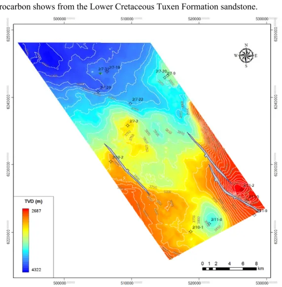
The depth structural map at the base of Cretaceous chalk inherited structural geometry from the BCU, however, the southern sub-sag has been shrunk drastically (Figure 14). The 2/7-31 well is located in a minor anticline and encountered hydrocarbon shows from the Lower Cretaceous Tuxen Formation sandstone.

(37)

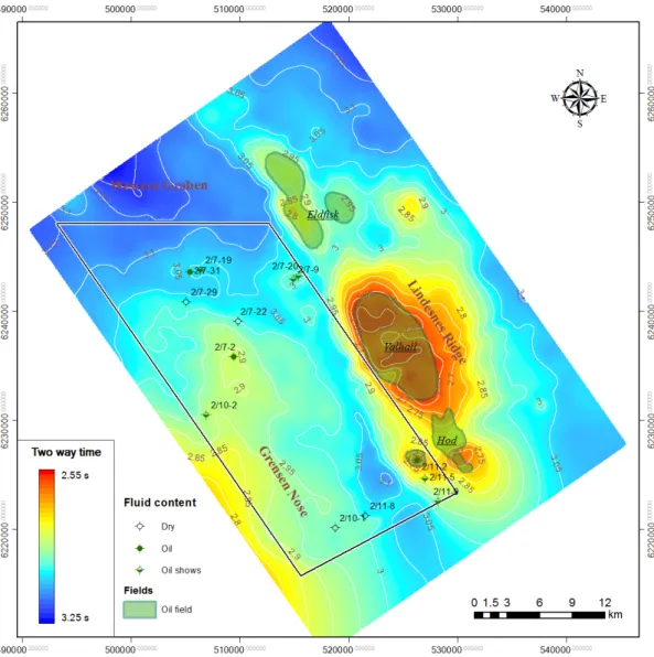
At least three four-way closures had been developed by salt diapirism on the depth structural map of Top Cretaceous (Figure 15). Hydrocarbons were tested from Cretaceous chalks, such as the 2/7-2 well, Embla Field (2/7-9 well located), and Hod Field (2/11-2 well located). In the Hod Field, the 2/11-5 and 2/11-9 wells were drilled below oil-water contact. Occasional hydrocarbon shows were reported from the 2/7-19 and 2/10-2 wells, where no significant closures were developed. These minor fingerprints from hydrocarbon shows can be explained by hydrocarbons having migrated through fractures or pores within chalk reservoirs and then escaped to shallower layers.

(38)

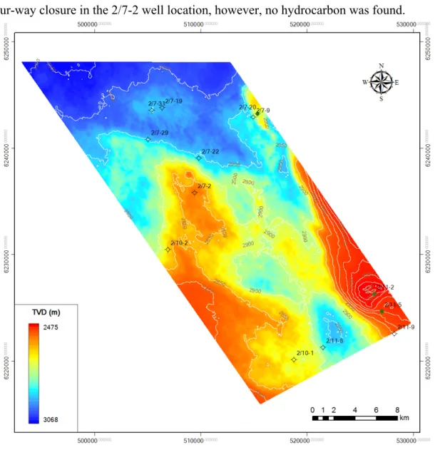
The buried depth of Paleocene Top Balder Formation ranges between 2475 and 3068 m (Figure 16). Hydrocarbon was reported from the 2/7-9, 2/11-2, and 2/11-5 wells, which are located in four-way anticlines induced by salt. There is a low-relief four-way closure in the 2/7-2 well location, however, no hydrocarbon was found.

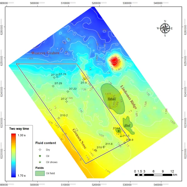
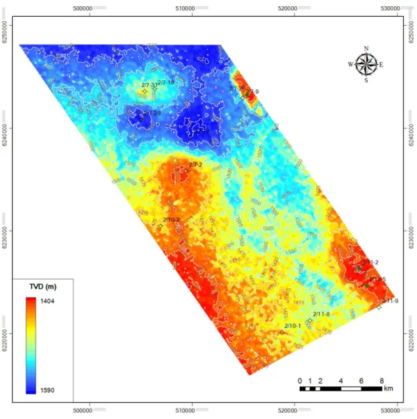
Figure 16. Depth-structure contour map of Top Balder Formation, Paleocene The top of Paleogene has a 186 m of relief (1404-1590 m) throughout the structure. Hydrocarbons were encountered in salt-induced anticlines, which comprise more than 50 m of relief. Enormous tortoise-shell pattern faults had been developed in the shallower sections while rifting, and they produced dense and irregular features on the grid of contour structural map (Figure 17).

(39)

Figure 17. Depth-structure contour map of Top Shetland Group, Paleogene

According to the relationship between discovered wells and seismic interpretation, it is concluded that:

(1) For the clastic sections beneath the BCU, hydrocarbons had been found in either structure-related faulted blocks or stratigraphy-entrapped closures; and

(2) For the strata above the BCU, hydrocarbons were generally preserved by salt-induced closures.

Consequently, it is necessary to perform seismic attribute analysis to characterize fluid responses and explore favorable petroliferous prospects.

(40)

5 Low-frequency seismic analysis

5.1 Low-frequency spectra

The ISA cube is constructed with the idea that constituting a series of spectral sections, which contain variable frequencies along specific seismic lines, either inline or crossline direction. In practice, users define the increment of frequency increment, and spectral sections can be produced for each individual frequency. Eventually, these spectral sections can be integrated into a cube. In an ISA cube, one direction displays the instantaneous spectrum of a certain frequency, the other direction shows instantaneous spectra along increasing frequencies.

ISA cubes are generated for seismic lines crossing penetrated wells, frequency are observed from 2 to 15 Hz, and the step of frequency increment is 1 Hz.

The 2/7-2 well tested hydrocarbons from Late Cretaceous Tor Formation (see green symbol in Figure 18a). On the ISA gather crossing the well, significant amplitudes are observed from 6 to 15.5 Hz. The maximum magnitude of attribute peak is listed in Table 2, the same as the rest of wells.

The 2/7-9 well tested hydrocarbon from Devonian sands, and recorded oil shows from the Late Cretaceous Ekofisk Formation chalk reservoirs. The significant amplitudes are observed from 3 to 15.5 Hz. The attribute peaks for above reservoirs appear at 7 and 11 Hz, respectively (Figure 18b).

(Figure to be continued)

5 10 15

4 6 7 8 9 11 12 13 14

Frequency (Hz)

(a) Inline2522 ISA gather across 2/7-2 well

3.0 3.5 TW T (ms) 0.563 3000 Stratigraphy Paleogene Cretaceous Permian 2 3 4 5 6 7 8 9 10 11 12 13 1415 Frequency (Hz)

(b) Inline3208 ISA gather across 2/7-9 well

3.5 4.0 TW T (ms) 0.00 800 Stratigraphy Paleogene Cretaceous Devonian 2 3 3.0

(41)

(Figure to be continued)

5 10 15

4 6 7 8 9 11 12 13 14

Frequency (Hz)

(c) Inline2688 ISA gather across 2/7-19 well

3.5 4.0 TW T (ms) 0.726 3750 Stratigraphy Paleogene Cretaceous Permian 2 3 3.0 Jurassic 5 10 15 4 6 7 8 9 11 12 13 14 Frequency (Hz)

(d) Inline2700 ISA gather across 2/7-22 well

3.5 TW T (ms) 0.829 1600 Stratigraphy Paleogene Cretaceous Permian 2 3 3.0 2.5 5 10 15 4 6 7 8 9 11 12 13 14 Frequency (Hz)

(e) Inline2466 ISA gather across 2/7-29 well

(f) Inline2618 ISA gather across 2/7-31 well

(g) Inline2410 ISA gather across 2/10-1S well

3.0 3.5 TW T (ms) 0.526 2600 Stratigraphy Paleogene Cretaceous Permian 2 3 2.5 5 10 15 4 6 7 8 9 11 12 13 14 Frequency (Hz) 3.0 3.5 TW T (ms) Stratigraphy Paleogene Cretaceous Permian 2 3 2.5

(h) Inline2112 ISA gather across 2/10-2 well

0.347 3500 5 10 15 4 6 7 8 9 11 12 13 14 Frequency (Hz) 1.5 TWT (ms) Stratigraphy Paleocene Cretaceous 2 3 2.0

(i) Inline3190 ISA gather across 2/11-2 well

0.000 2500 Eocene 2.5 3.0 1.0 5 10 15 4 6 7 8 9 11 12 13 14 Frequency (Hz) TW T (ms) Stratigraphy Paleogene Cretaceous Permian 2 3 Jurassic

(j) Inline3156 ISA gather across 2/11-5 well

0.000 2500 3.0 2.0 2.5 1.5

(42)

Figure 18. ISA gather with frequencies from 2Hz to 15 Hz at the well location ( : oil tested; : oil shows recorded)

The 2/7-19 well tested hydrocarbon from the Late Jurassic Ula Formation sandstone, and recorded oil shows from Late Cretaceous Hidra Formation and Tor Formation chalk reservoirs. Significant amplitudes for the Late Jurassic pay zone are observed from 3 to 10 Hz. The attribute peaks for above reservoirs appear at 7 , 8, and 13 Hz, respectively (Figure 18c).

The 2/7-22 well tested hydrocarbon from Devonian sands. significant amplitudes for the pay zone are observed from 6 to 15Hz, and the attribute peaks for the reservoirs appear at 15 Hz (Figure 18d).

The 2/7-29 well tested hydrocarbon from the Late Jurassic Eldfisk Formation sandstone. Significant amplitudes for the pay zone are observed from 4 to 15 Hz, and the attribute peak appears at 5 Hz (Figure 18e).

The 2/7-31 well tested hydrocarbon from Late Jurassic Ula Formation sands, and recorded oil shows from Early Cretaceous Tuxen Formation chalk and Early Permian Rotliegendes sandstone. Significant amplitudes for the pay zones are observed from 6 to 15 Hz, and the attribute peaks for above reservoirs appear at 11, 9, and 11 Hz, respectively (Figure 18f).

The 2/10-1S well encountered a gas kick from Permian Rotliegendes sandstone. Significant amplitudes for Rotliegendes sand are observed from 6 to 14 Hz, and the attribute peaks for the reservoir appears at 10 (Figure 18g).

5 10 15 4 6 7 8 9 11 12 13 14 Frequency (Hz) 3.5 TW T (ms) Stratigraphy Paleogene Cretaceous Permian 2 3 3.0

(k) Inline2648 ISA gather across 2/11-8 well

0.677 3500 2.5 5 10 15 4 6 7 8 9 11 12 13 14 Frequency (Hz) 3.5 TW T (ms) Stratigraphy Paleogene Cretaceous 2 3 3.0

(l) Inline3144 ISA gather across 2/11-9 well

0.000 4500 2.5

(43)

The 2/10-2 well reported oil shows from Late Cretaceous Tor Formation chalk reservoirs. Significant amplitudes for the reservoirs are observed from 4 to 15 Hz, and the attribute peak appears at 12 Hz (Figure 18h).

The 2/11-2 well tested hydrocarbon from Late Cretaceous Hod Formation chalk and Paleocene Hordaland Group clastic reservoirs. Significant amplitudes for the pay zones are observed from 3 to 15 Hz, and the attribute peaks for above reservoirs appear at 5 and 8 Hz, respectively (Figure 18i).

The 2/11-5 well encountered oil shows from Late Cretaceous Ekofisk Formation chalk and Paleocene Hordaland Group clastic reservoirs. Significant amplitudes for reservoirs are observed from 3 to 15 Hz, and the attribute peaks for above reservoirs appear at 9 and 6 Hz, respectively (Figure 18j).

Although two attribute peaks show on the ISA gather across the 2/11-8 well, there was no hydrocarbon was encountered and reported. These attribute anomalies might be related to variation of fluid saturation between different lithologies (Figure 18k).

The 2/11-9 well recorded oil shows from Late Cretaceous Ekofisk Formation chalk reservoirs. Significant amplitudes for the reservoir are observed from 4 to 15 Hz, and the attribute peak appears at 12 Hz (Figure 18l).

The above observations conclude that low-frequency spectra show significant indications of when reservoirs are saturated with hydrocarbon. However, it is difficult to designate one or two frequency bands to be the best representation specifically. Instead, all bands from low-frequency range (< 15 Hz) may have potential probabilities of showing abnormal frequency responses.

(44)

30

Table 2. Attribute peaks on petroliferous sections across key wells

No. Well ISA volume Content Petroliferous section Attribute peak

Inline Crossline Age Group/Formation Frequency Numeric magnitude

1 2/7-2 2522 Oil Late Cretaceous Tor Fm 15Hz 2764

2 2/7-9 3208 Oil Devonian 7Hz 523

Oil shows Late Cretaceous Ekofisk Fm 11Hz 617

3 2/7-19 2688 3306

Oil Late Jurassic Ula Fm 7Hz 3630

Oil shows Late Cretaceous Hidra Fm 8Hz 2749

Tor Fm 13Hz 3828

4 2/7-22 2700 Oil Devonian 15Hz 970

5 2/7-29 2466 3176 Oil Late Jurassic Eldfisk Fm 5Hz 3332

6 2/7-31 2618

Oil Late Jurassic Ula Fm 9Hz 1933

Oil shows Early Cretaceous Tuxen Fm 11Hz 3837

Oil shows Early Permian Rotliegendes Gp 11Hz 1766

7 2/10-1S 2410 Gas shows Permian Rotliegendes Gp 10Hz 1988

8 2/10-2 2112 Oil shows Late Cretaceous Tor Fm 12Hz 3307

9 2/11-2 3190 Oil Late Cretaceous Hod Fm 5Hz 1645

Oil Paleocene Hordaland Gp 8Hz 4617

10 2/11-5 3156 Oil shows Late Cretaceous Ekofisk Fm 9Hz 1822

Oil shows Paleocene Hordaland Gp 6Hz 2744

11 2/11-8 2648 Dry

12 2/11-9 3144 Shows Late Cretaceous Ekofisk, Tor and Hod Fm 12Hz 4430

(45)

31

5.2 Frequency responses on wells

To illustrate the relationship between low-frequency shadow effects and fluid mobility, it is critical to find evidence from spectral sections through discovered wells.

Spectral profiles for the 2/7-2, 2/7-19, 2/7-22, 2/7-29, and 2/7-31 wells along the crossline direction of the seismic survey were extracted. For the 2/10-2 well, the profile was extracted along the inline direction (Figure 19).

Figure 19. Seismic lines for spectral sections through key wells

0 2 4 6 8 10 km 500000 510000 520000 530000 490000 62 50 00 0 62 4 00 00 6 23 00 0 0 62 20 00 0 500000 510000 520000 530000 490000 62 50 00 0 62 4 00 00 6 23 00 0 0 622 0 00 0 North 2/7-9 2/7-19 2/7-31 2/7-29 2/7-22 2/7-2 2/10-2 2/10-1S 2/11-8 2/11-9 3D volume Oil discovery Gas shows Oil shows Dry hole 2/11-5 2/11-2 XL26 50 IL 21₁₂ Xl28 40 Xl31 78 Xl33 10 Xl33 46

(46)

32

The 2/7-2 well tested hydrocarbon in the uppermost part of the Late Cretaceous Tor Formation with more than 40% of water after acidization. The pay zone shows amplitude anomalies on the 12, 15.5, and 20 Hz spectral sections (Figure 20). Amplitude anomaly for pay zone faded out on the 30 and 40 Hz spectral sections, and the amplitude anomaly appears below the pay zone on the 40 Hz section.

Crossline2650 TWT (s ) 3.0 3.5 4.0 Normal po larity Top K B CU Oi l +933.95 000. 00 -933.95 300 0 400 0 50 0 0 0 500 00 0 80 0 Crossline2650 TWT (s ) 3.0 3.5 4.0 Frequency 12 Hz Top K B CU Oi l TWT (s ) 3.0 3.5 Frequency 2 0Hz Top K B CU Oi l TWT (s) 3.0 3.5 Frequency 15.5Hz Top K B CU Oi l TWT (s) 3.0 3.5 Frequency 30Hz Top K B CU Oi l TWT (s ) 3.0 3.5 Frequency 4 0Hz Top K B CU Oi l

(47)

33

The 2/7-19 well tested hydrocarbon in the Upper Jurassic Ula Formation. The pay zone shows amplitude anomalies on the 12 and 15.5 Hz spectral sections (Figure 21). Amplitude anomaly for pay zone faded out on the 20, 30, and 40 Hz spectral sections, but the amplitude anomaly appears either above or beneath the pay zone on these sections.

(48)

34

The 2/7-22 well tested hydrocarbon in the Devonian alluvial clean sands. The pay zone is located on the edge of anomalies on the 12, 15.5, and 20 Hz spectral sections (Figure 22). Amplitude anomaly for pay zone persists to higher frequency sections, such as 30 and 40 Hz, but the amplitude anomaly appears above the pay zone on these sections.

Crossline2840 TWT (s ) 3.0 3.5 4.0 Normal po larity Top K B CU Oi l +933.95 000. 00 -933.95 680 0 350 0 50 0 0 0 500 00 0 80 0 Frequency 12 Hz Frequency 2 0Hz Frequency 15.5Hz Frequency 30Hz Frequency 4 0Hz Crossline2840 TW T (s) 3.0 3.5 4.0 Top K BC U O il TW T (s) 3.0 3.5 4.0 Top K BC U O il TW T (s ) 3.0 3.5 4.0 Top K BC U O il TW T (s ) 3.0 3.5 4.0 Top K BC U O il TW T (s) 3.0 3.5 4.0 Top K BC U O il

(49)

35

The 2/7-29 well tested hydrocarbon in the Devonian alluvial clean sands. The pay zone is located on the edge of anomalies on the 7.2 and 15.5 Hz spectral sections (Figure 23). Amplitude anomaly for pay zone faded out on the 20, 30, and 40 Hz spectral sections, but the amplitude anomaly appears above the pay zone on these sections.

Crossline3178 TWT (s ) 3.0 3.5 4.0 Normal po larity Top K B CU Oi l +933.95 000. 00 -933.95 680 0 350 0 50 0 0 0 500 00 0 80 0 Frequency 7 .2 Hz Frequency 2 0Hz Frequency 15.5Hz Frequency 30Hz Frequency 4 0Hz Crossline3178 T WT (s ) 3.0 3.5 4.0 Top K B CU Oil TWT (s ) 3.0 3.5 4.0 Top K B CU Oi l T WT (s ) 3.0 3.5 4.0 Top K B CU Oil TWT (s ) 3.0 3.5 4.0 Top K B CU Oi l T WT (s ) 3.0 3.5 4.0 Top K B CU Oil

(50)

36

The 2/7-31 well tested hydrocarbon in the Upper Jurassic Ula Sandstone. The pay zone is located on the edge of anomalies on the 12 and 15.5 Hz spectral sections (Figure 24). Amplitude anomaly for pay zone faded out on the 20, 30, and 40 Hz spectral sections, but the amplitude anomaly appears both above and below the pay zone on these sections.

Crosslin e3346 TWT (s ) 3.0 3.5 4.0 Normal po larity Top K B CU Oi l +933.95 000. 00 -933.95 600 0 350 0 50 0 0 0 500 00 0 80 0 Frequency 12 Hz Frequency 2 0Hz Frequency 15.5Hz Frequency 30Hz Frequency 4 0Hz Crossline3346 TW T (s) 3.0 3.5 4.0 Top K BCU O il TWT (s ) 3.0 3.5 4.0 Top K B CU Oi l TW T (s) 3.0 3.5 4.0 Top K BCU O il TWT (s ) 3.0 3.5 4.0 Top K B CU Oi l TW T (s) 3.0 3.5 4.0 Top K BCU O il

(51)

37

The 2/10-2 well encountered Late Cretaceous Tor Formation, and there are no significant amplitude anomalies on spectral sections for chalk reservoir zones (Figure 25).

Figure 25. IL2112 spectral sections corresponding to the stacked seismic profile

Inline2112 TWT (s ) 2.5 3.0 3.5 Normal polarity Top K O il shows +933.95 000. 00 -933.95 800 0 500 0 100 0 0 0 600 00 0 150 0 B CU Inline2112 TW T (s) 2.5 3.0 3.5 Frequency 9.4Hz Top K Oi l shows BC U TWT (s ) 2.5 3.0 3.5 Frequency 1 2Hz Top K O il shows TW T (s) 2.5 3.0 3.5 Frequency 20Hz Top K Oi l shows TWT (s ) 2.5 3.0 3.5 Frequency 3 0Hz Top K O il shows TW T (s) 2.5 3.0 3.5 Frequency 4 0Hz Top K Oi l shows B CU BC U B CU BC U

(52)

38

The significant amplitudes spectral profiles show that low-frequency seismic presents significant anomalies for the fluid saturated sections, and high-frequency signals attenuated while propagating through pay zones. Consequently, considering amplitude anomaly features for further prospects, possible pay zones can be identified based on the following conditions:

(1) Low-frequency spectra often show amplitude anomalies; (2) High-frequency spectra are usually attenuated drastically; and

(3) Amplitude anomalies may appear either above or below or to the side of petroliferous sections.

(53)

39

5.3 Frequency responses along horizons

To analyze frequency responses along the BCU, Top Cretaceous, and Top Paleogene, significant amplitudes attributes have been extracted from time-frequency envelopes of 4.8, 7.2, 9.4, 12, 15.5, 20, 30, 40, and 50 Hz. Each slice calculated the mean value of the envelope within a specific window, for instance, 200ms was involved below the BCU, 200ms was designated below Top Cretaceous, and 180ms was considered below Top Paleogene.

Considering penetrated wells show various attribute peak responses from arbitrary frequency range in pay zones, frequency attribute slices were classified into three categories, which are low-frequency attribute, medium-frequency attribute, and high-frequency attribute.

The low-frequency attribute slice was integrated by attributes of 4.8, 7.2, 9.4, 12, and 15.5 Hz slices, and it was normalized with the following algorithm:

1

5 4.8, 7.2, 9.4, 12, 15.5

The medium-frequency attribute slice comprises attributes of 20 and 30 Hz slices, and it was normalized with the following algorithm:

1

2 20 30

The high-frequency attribute slice was computed by 40 and 50 Hz slices, and it was normalized with the following algorithm:

1

2 40 50

Consequently, each horizon has three attribute slices to demonstrate frequency responses.

(54)

40 5.3.1 BCU frequency responses

The low-frequency attribute slice shows several strong responses. Existing wells are located in these abnormal areas, such as the 19, 22, 29, and 2/7-31 wells (Figure 26). The Embla oil field was discovered by the 2/7-9 and 2/7-20 wells, even though these two wells are located in weak responses area, which was caused by poor seismic data quality due to gas interference. Although the 2/10-2 well is plotted on the edge of a strong response, the well is located on the up-thrown side of a normal fault (Figure 29). The 2/10-1 well reported a gas kick in Permian Rotliegendes sands, and it did not show any significant abnormal responses.

(55)

41

The medium-frequency attribute slice shows similar responses with previous low-frequency attribute slice. But there are more pronounced anomalies present in the southern corner of seismic volume. In addition, the region west of the 2/10-2 well has the strongest responses (Figure 27).

Figure 27. Medium-frequency attribute within 200ms below BCU

Frequency anomalies are weaker in the northern part of seismic volume in the high-frequency attribute slice (Figure 28), however, similar responses still remain in several areas, such as the east of the 2/7-22, west of the 2/7-2, and east of the 2/10-2,

(56)

42

which are considered to be favorable exploration prospects. The area between the 2-11-8 and 2/11-6 wells vanished completely.

Figure 28. High-frequency attribute within 200ms below BCU

The low-frequency anomalies below the BCU (Figure 26) were plotted on the structural map of the overlying BCU. These anomalies distribute along the slope of the northern sub-sag or inside the depocenter of the southern sub-sag (Figure 29).

Upper Jurassic source rock, Kimmeridgian shale was deposited in the depocenter of the southern sub-sag. The low-frequency responses within this region might be directly produced by hydrocarbon generated from the hot shale.

(57)

43

Figure 29. BCU structural map overlying low-frequency anomalies (Faults are shown with grey polygons)

5.3.2 Late Cretaceous frequency responses

Although several wells encountered hydrocarbons in Upper Cretaceous chalk reservoirs, the low-frequency attribute slice does not show exciting coincidence between frequency responses and fluid content of wells (Figure 30). The 2/11-2 well from the Hod oilfield is located in seismic obscured area, and does not show abnormal responses. The same problem appears in both the 2/7-9 well located Embla field and

(58)

44

the Valhall field. Instead, on the rim of the Valhall and Hod fields, frequency attribute illustrates strong responses, which might be caused by residual oil around anticlines.

Furthermore, there is a widespread abnormal cloud to the west of the 2/7-2 well, and this location shows similar anomaly in the BCU frequency attribute slices.

Figure 30. Low-frequency attribute within 200ms below Top Cretaceous

The medium-frequency attribute slice has inherited responses from the low-frequency responses (Figure 31). In comparison, the magnitude of the response to the west of the 2/7-2 well has been amplified, and instead, the responses surrounding existing oilfields have been weakened.

(59)

45

Figure 31. Medium-frequency attribute within 200ms below Top Cretaceous

The frequency responses on the rim of existing oilfields are eliminated on the high-frequency attribute slice, while the anomaly to the west of the 2/7-2 west still remains strong (Figure 32).

(60)

46

Figure 32. High-frequency attribute within 200ms below Top Cretaceous

Plotting the low-frequency anomalies below Top Cretaceous (Figure 30) onto the Top Cretaceous structural map, abnormal responses are seen distributed along the slope of the sub-sags or on the flank of Grensen Nose (Figure 33). The west of the 2/7-2 well and the western flank of the Lindesnes Ridge are regarded as favorable exploration targets for hydrocarbon saturated chalk reservoirs.

(61)

47

Figure 33. Top Cretaceous structural map overlying low-frequency anomalies 5.3.3 Late Paleogene frequency responses

In the shallow sections, hydrocarbons were discovered within Late Eocene clastic sands. The Hod oilfield displays strong frequency responses on the low-frequency attribute slice, and some sparkle anomalies appear in the Embla oilfield (Figure 34). The rest region is poor with frequency responses, which is corresponding to brine saturated reservoirs of penetrated wells.

(62)

48

Figure 34. Low-frequency attribute within 180ms below Top Paleogene

The medium-frequency attribute slice shows slightly increasing area of anomalies, however, no significant area is expected for the purpose of petroleum exploration (Figure 35).

(63)

49

Figure 35. Medium-frequency attribute within 180ms below Top Paleogene

The high-frequency attribute slice (Figure 36) shows similar responses with the previous segments (Figure 34 and Figure 35). The magnitude from responses in the middle of Hod field is much lower than that from the rim, which can be explained by the hydrocarbons being concentrated within the uppermost cap of the anticlines, and high-frequency energy attenuated while penetrating through massive chalk reservoirs.

(64)

50

Figure 36. High-frequency attribute within 180ms below Top Paleogene

Plotting the low-frequency anomalies below Top Paleogene (Figure 34) onto the Top Paleogene structural map, anomalous response distribution is overlying the anticline (Figure 37). Considering no significant abnormal responses are characterized within the under-exploration area, no further prospects are recommended for the shallow sections.

(65)

51

(66)

52

5.4 Prospect identification

5.4.1 BCU prospects

The low-frequency seismic detected 96 km2_{of abnormal responses beneath} the BCU. Responses within polygon C, D, F, and G are bounded by normal faults, while the rest, A, B, E, H, and I, are stratigraphy related (Figure 38).

Figure 38. BCU clastic-reservoir polygons from low-frequency attribute slice

On conventional time-domain stacked seismic profiles, several bright spots with strong reflections beneath BCU indicate possible geo-bodies, which may comprise porous reservoirs. Such events are observed on frequency-domain seismic

(67)

53

sections crossing existing wells, e.g. the 2/7-29, 2/7-19, 2/7-22, and 2/7-31 wells, where hydrocarbons flowed from field tests. For instance, the 2/7-31 well penetrated a fault-bounded closure and tested hydrocarbon from Upper Jurassic Ula Sandstone, and strong frequency responses appear on the 10 Hz spectral section (Figure 39; line location see Figure 38 inline 2620). The downthrown side responses to the northwest direction have been tested by the 2/7-29 well, which obtained a one-gallon dead-oil sample in the Upper Jurassic Eldifisk Formation sandstone.

Figure 39. 10 Hz spectral section corresponding to the stacked seismic profile

Top K B CU Oi l Base chalk B al der Fm. 2.5 3.0 3.5 4.0 4.5 TW T (S) 2/7-31 NW SE 400 0 Top K B CU Oi l Base chalk B al der Fm. 2.5 3.0 3.5 4.0 4.5 TW T (S) 2/7-31 _Inline2620 Frequency: 10Hz NW SE 2/7-29 area

(68)

54

On the flank of the Grensen Nose, there are several high-amplitude reflections on the stacked seismic, and strong responses are shown on the low-frequency envelope. These anomalies lie beneath the BCU, and possibly indicate the presence of hydrocarbons (Figure 40; line location see Figure 38 inline 2236). This type of reflection shows the same play concept with existing wells, e.g. the 2/7-31 well, which provides exciting evidence of hydrocarbon existence. Similar abnormal low-frequency spectra can be identified from polygon A, B, D, F, and G of the BCU prospect map (Figure 38), and the total coverage for these polygons is 43 km2_{. The} reservoir rock for these prospects is considered to be composed of sandstone from Upper Jurassic, Permian, or Devonian.

Figure 40. 8 Hz spectral section corresponding to the stacked seismic profile

2.5 3.0 3.5 4.0 4.5 TW T (S) NW SE Inline2236 2.5 3.0 3.5 4.0 4.5 TW T (S) NW SE Frequency: 8Hz Top K B CU Base chalk B al der Fm. Top K B CU Base chalk B al der Fm. 400 0 prospect