Splatting multiresolution volume data using the Feature Graph

Splatting multiresolution volume data using the Feature

Graph

J. Campos1& A. Puig1& D. Tost2

1_{University of Barcelona, Spain} 2_{Politechnical University of Catalonia, Spain}

Abstract

We propose to represent classified datasets as a feature graph storing different graphical models and attributes for each feature. This graph allows us to render each feature according to its own characteristics. In addition, we show that various features of the graph storing volume information at different resolution levels can be rendered together using a view-aligned splatting method. Moreover, we propose a 2D kernel function for splats that is easy to tune and generates smaller footprints that reduce the render time. Our algorithm provides images with less blur. It enhances the boundary of the features while avoiding the subdivision of homogeneous regions of the volume.

Categories and Subject Descriptors(according to ACM CCS): I.3.3 [Computer Graphics]: Viewing algorithms

1. Introduction

In scientific visualization, there is a growing interest for the visual and semantic quality of the rendered images and for the interfaces through which users specify the set of visu-alization parameters [vW05]. Classification has been recog-nized [Pa01] as one of the major issues in visualization. It is indeed an important step of data exploration, because it is used to determine which materials are at every sampled position. However, the visualization problems do not finish once a dataset has been classified. On the contrary, a true tal-ent of graphical design and skills in illustration are necessary to obtain meaningful images of a pre-classified dataset, im-ages that emphasize relevant focused structures while keep-ing some details of the context surroundkeep-ing elements. This is precisely one of the current problems of visualization: the design of the images is delegated to users of visualiza-tion applicavisualiza-tions, scientists and physicians who, generally, do not have the required graphical skills for it, and, more-over are more-overwhelmed by the complexity of the interfaces. This is why many efforts are now being done to provide vi-sualization software with mechanisms that ease or automa-tize the computation of rendering parameters such as cam-eras [BE06], transparency [GDF03] and sparsness [VKG05] of different features. On a large extent, these techniques rely

on a previous step of classification and segmentation of the different features of the dataset.

Depending on the methods chosen to render classified datasets, it may be necessary to design data structures that provide a direct access to the graphical model of each fea-ture. Examples of such structures are the lists of voxels used in two-level rendering (RenderLists [HMBG01] and ob-jects sets[HBH03]) and the run-length encoding the feature identifiers of the voxels for multimodal rendering [FPT06]. More complex topological representations of datasets based on their skeleton have also been proposed for animation [CSW∗03]. However, all these structures represent the same volumetric information for all the features. Other structures such as octrees [WG94] support different levels of resolu-tion, but, since they are based on a spatial subdivision of space, they are not convenient to separate segmented struc-tures.

In this paper, we propose to represent datasets as a graph of features providing direct access to each feature. The fea-tures can be represented with a different model and at a different resolution level. Thus, they can be rendered sep-arately according to their own characteristics. When differ-ent features are rendered together, two main problems must be solved: occlusion and transition between features. In this paper, we address the rendering of features represented by

voxels at different resolutions. We use a view-aligned splat-ting algorithm capable of handling voxels of different sizes. In addition, we propose to compute the voxels splat using as kernel function a beta function that is easy to tune and generates smaller footprints that reduce the render time. Our algorithm provides images with less blur. It enhances the boundary of the features while avoiding the subdivision of homogeneous regions of the volume.

2. Related work

Data structures for the representation of classified datasets

Most spatial decomposition data structures used in volume rendering, such as pyramids [LH91], octrees [DKC00] and BSP trees [LMK03], have been designed to provide space leaping mechanisms and to compress volume data. How-ever, less bibliography address the problem of represent-ing segmented and pre-classified ortagged data. Tiede et al. [TSH98] propose to use together with the original voxel model an additional volume containing an identifier (ID) of the region to which each voxel belongs. The drawback of this approach is that it does not provide a direct access to the features. Ferré et al. [FPT06] partially solve this problem by using a run-length codification of the voxels identifiers which can be used to skip non selected features during ren-dering. A direct representation of the features are the Ren-derLists[HBH03]) used for two-level rendering. This struc-ture stores lists of voxels of all the feastruc-tures for each slice of the volume. It supports only disjoint features of the same resolution. An alternative idea is to partition the voxel model into sub-models, hence preserving the spatial ordering of the voxels inside the sub-models. Specifically, Li et al [LMK03] use disjoint boxes to ease depth sorting. Puig et al. [PTN00] support overlapping voxel models, because these sub-models are organized in a graph that drives the data traver-sal. This graph represents the limbs and joints of the cere-bral vascular structure that are supposed to be disjoint so that each voxel sub-model masks the overlapping ones. Finally, for volume animation and deformation, Singh et al. [SSC03] and later Walton et al. [WJ06] represent topological skele-tons of the human body that associate voxel sub-models to each segment of the skeleton. All these approaches represent disjoint features, with the same resolution. Our goal is pro-vide a structure capable of handling non-disjoint features, each of them with its own convenient resolution.

Splatting tagged volumes

One of major advantages of splatting is that reduces sig-nificantly aliasing because of the smooth kernels decay [Wes89]. Unfortunately, this smooth decay and the kernels’ overlapping at the edges produce blurred boundaries. Sev-eral methods have been proposed to overcome this draw-back. Mueller et al. [MMC99] use of a post-shade scheme

instead of the traditional pre-shaded approach. However, generally, post-shading has a higher cost than pre-shading because it projects a larger number of voxels and performs shader more times per voxel. Huang et al. [HCS98] employ different kernels depending on the proximity of voxels to edges and the strength of those edges. This method is ef-fective for iso-surface edges, but not for micro-edges within the iso-range. Meredith and Ma [MM01] use a multition octree. For each node, they choose the coarser resolu-tion and check if its corresponding splat size on screen is below a given threshold. If it is greater than the threshold, they descend to a finer resolution. This way, they avoid both aliasing and blurring by choosing the largest splats when-ever it is possible without blur. Birkfellner et al. [Ba05] use smaller kernels to minimize the blurring artifacts, and dis-place stochastically the voxels positions to avoid that the splats follow aligned patterns.

In addition, in the visualization of tagged volumes the determination of ID boundaries at subvoxels resolution causes aliasing effects. Both problems have been addressed in the bibliography in the context of ray-casting [TSH98] [KCOY03] and texture mapping [VHN∗05]. Mueller et al. [MLK03] do not work explicitly with tagged volumes, but they identify voxels of the different regions of interest (ROI) of a dataset and migrate their density range to private inter-vals. They apply intensity-flipping at the transition between features achieving a smooth decay at the boundaries. How-ever, this approach is hard to extend to tagged data, seg-mented using more criteria than the property range only.

Finally, for perspective projections, Mueller et al. [MMI∗98] propose to use different kernel sizes according to the distance to reduce perspective aliasing. Zwicker et al. [ZPvBG01] applyelliptical weighted average non uni-form kernels to provide different footprints and low-pass lev-els depending on the distance from the observer.

In our approach, features are represented at a convenient resolution. Specifically, we represent surface features, i.e features representing regions boundaries at a higher resolu-tion than internal regions. Thus the boundary splats are natu-rally smaller than the others, which reduces blurring. More-over, our model handles various levels of resolution for each feature. Therefore, if a feature is far from the viewer or it is out of the user focus, a coarser resolution is used and it is rendered blurry. On the contrary, higher resolution are used for focused features. This reduces the aliasing of perspective projection and provides focus+context visualizations.

3. The Multi-resolution Feature Graph Definition

Our model represents classified voxel models. The classifi-cation can be done according toncdifferent non-exclusive criteria that can be expressed as boolean conditions. There-fore, after classification, for each voxelv, we have a set of

ncboolean values(labels) ri(v),i= [1..nc]that indicate if the voxel fulfils or not each boolean expression. As an example, if the classification criteria are: bone, fat, arm, leg and toe, a voxel of the toe bone will have the following labels (1, 0, 0, 1, 1), as it also belongs to the leg.

The voxel model can be clustered into different sets ac-cording to any combination of these labels. Although the theoretical number of clusters is 2nc, in fact, many of them are empty because all the combinations are not possible. In our example, possible clusters are: “bone”, “bones and toe”, “fat and arm” , but the cluster “bone and fat” is empty. We define the concept offeatureas a non-empty cluster. More precisely, afeature(f) is a set of values for a subset of the boolean expressions used in the classification such that at least one voxel of the model fulfills these expressions. We can associate to any feature the set of voxels of the volume that have the same label values. Then, sets of voxels of a fea-ture can be totally or partially included into sets of voxels of other features. In our example, the set of voxels of the fea-ture “bone and toe” is totally included in the set of voxels of features “bone” “toe”.

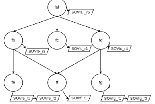
We represent the features and the inclusion relationship as a graph. Specifically, theFeature Graphis a directed acyclic graph such that each node represents a feature and each arc represents the relationship of inclusion of the corresponding sets of voxels. The direction of the arcs goes from the larger to the smaller included feature. The entry point to the graph is a feature (fall) that includes all the features that do not have an ancestor. The leaf nodes of the graph correspond to features that do not include any other feature. Each feature of the graph has its own optical properties used for rendering. Finally, in order to provide a direct index to the feature nodes of the graph model, we use aFeature Hash Table.

fc fb fd fall fe ff fg SOVfall_r5 SOVfd_r4 SOVfc_r1

SOVfe_r1 SOVfe_r2 SOVff_r1 SOVfg_r1 SOVfg_r3 SOVfb_r3

Figure 1: TheFeature Graph that provides direct access to the data models associated to each feature, which can be at stored at different resolutions.

Sets of voxels

We define the set of voxels of a feature asSOV(fi). Since the

SOV of the leave nodes are disjoint and are totally included

in theSOVof their ancestors, in order to avoid redundancies, we only storeSOVs in the leaf nodes of the graph. Then, the

SOV of an intermediate feature can be obtained by recur-sively traversing its descendant nodes down to the leaves. Voxels of theSOVs can be represented either as submodels of voxels or voxels lists. In the former case, although the

SOV sare disjoint, their bounding box can overlap. We as-sign a zero value to the voxels of a submodel that do not belong to the feature, so that a voxel has a non-zero value in only one unique leaveSOV. This way, spatial ordering in-sideSOV sis preserved. This representation is convenient if the voxels distribution is compact. In the second case, the access to the voxels of a feature is direct, it is not necessary to traverse its submodel and check for the property value. It is convenient when the features are sparse and spread in the volume. As a drawback, it is necessary to store the voxels coordinates and there is no spatial ordering inside theSOV. Accordingly, we choose the type ofSOV representation ac-cording to the spatial distribution of the feature and to the rendering algorithm.

The homogeneous regions of a SOV can also be com-pacted using different voxel sizes. WhenSOV sare imple-mented as subvoxel models, this is done using an octree of each submodel. Alternatively, the list of voxels stores only the black nodes of the octree with their associated size. Fur-thermore, since theSOV scan be stored in different files, ef-ficient out-of-core traversal strategies can be applied.

Multiresolution

Because of its hierarchical nature, and because it clusterizes the voxels, theFeature Graph can handle multiresolution representations of the voxel model. To do so, we only need to compute the sets of labels at coarser levels of representations of the voxel model. It should be noted that some clusters that were non-empty at the higher resolution can become empty at a lower resolution. Therefore, not all the features of the higher resolution level exist at lower levels. Consequently, some features can be leaves at a resolution and intermedi-ate nodes at another resolution. Accordingly to our policy of avoiding redundancies, we store theSOV sonly at the leaves of each resolution level. At rendering time, when a resolu-tion level of a feature is required, the feature node that have the closest level of resolution in the selected hierarchy fea-ture is visualized.

Finally, each graph feature could be represented by differ-ent models, such as a surface model extracted from aSOV

and stored as a polygon list. A generic multiresolution Fea-ture Graphis shown in Figure1.

4. Graph Construction

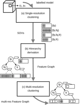
The construction of the Features Graph takes as input the set of voxels, labeled according to thenccriteria. It is composed of 3 steps: (a) the clustering of the voxels into sets of voxels

with identical labels, (b) the derivation of the features hier-archy -creation of the nodes and arcs of theFeature Graph-, and (c) a recursive compression through the graph hierarchy to obtain multiresolution sets. Figure2shows the schema of this construction process.

SOVs (fp) (fp,fq) (fp,fr) (fp,fq,fr) labelled model f1..fn Feature Graph

multi-res Feature Graph (b) Hirerarchy derivation (a) Single-resolution clustering (c) Multi-resolution clustering fp fq fr fp fq fr

Figure 2:Feature Graph Construction: (a) single resolution clus-tering (b) features hierarchy derivation, and (c) multiresolution clustering.

The clusters computed in the first step are actually the

SOV sof the leave features of the graph at the highest resolu-tion. To compute them, we traverse the labeled voxel model using the set of labels of each voxel as a hash code of the

Feature Hash Table. Each voxel is added to theSOVindexed by its hash code. At this point of the process, theSOV sare represented as lists of voxels. Once they are filled, we are able to compute their bounding box and to create a voxel submodel for each of them. These voxel submodels are com-pressed as octrees. Then, either the octrees are used directly to represent theSOV sor they are traversed to create a new list-based representation of theSOV swith voxels of various sizes.

In the second step of the process we construct the graph. First, we create the leave nodes and we associate to them the computedSOV s. Next, we derive the graph hierarchy through an iterative process based on boolean operations be-tween the feature labels. This process recursively creates common ancestor nodes for all the nodes that share a bit of their hash code. When the hierarchy is built, theFeature Hash Tableis updated to reference to new created nodes. At the end of the process, if the graph is composed of various

disconnected hierarchies, we create the feature(fall)as the common root.

Finally, we compute the sets of voxels at coarser levels of representations of the original voxel model and repeat the clustering process for larger voxels. Then, theSOV s com-puted with these coarser clusters of voxels are distributed through the graph hierarchy and attached to the correspond-ing nodes. Thus, each node can contain different resolution levelSOVs.

5. View-aligned splatting of the Feature Graph

Rendering the Feature Graph depends on how theSOVs are represented, as voxel sub-models or lists. In this paper, we focus on the second representation. Since lists do not pre-serve spatial ordering, we have chosen the view aligned splatting approach that transforms and inserts orderly the voxels in view-aligned buckets.

Graph traversal

The input of the rendering is a set of feature keys that have to be rendered calleduser query. In addition, user can spec-ify the resolution at which the selected features need to be rendered, or this resolution can be computed automatically depending on the ratio pixel/voxel of the projection and the feature’s distance to the camera view reference point.

The feature keys of the user query are used to access the

Feature Hash Tablein order to fetch the selected nodes of the graph. TheSOVs to be rendered are obtained by recur-sively traversing the selected features and their descendants. At each feature node of the graph, the selected resolution level is checked against the node resolution level. If the res-olution level of the node is the same or higher than the de-sired one, the voxels of theSOV associated to the node are view transformed and inserted into the sheet buffers. In the opposite case, the node descendants are recursively visited and the same procedure is applied again. The optical prop-erties applied for aSOV are inherited from the selected an-cestor feature node. Besides, as all of voxels of aSOVshare optical properties, they are set once at the beginning of each

SOVtraversal. Then, we iterate on the voxels of theSOVand we fill the sheet-buckets corresponding to the different voxel locations. Each voxel contribution to the volume rendering integral is defined by a set of kernel sections that fall within a set of cutting planes (sheet-buckets). A different set of kernel sections is computed for each footprint size defined by each resolution value. Pre-integrated kernel sections are used for fast rasterization and each sheet-bucket position stores the corresponding kernel index. At the end of the selected fea-tures traversal, the composition of all sheets or buckets in FTB order is performed.

Splatting kernels

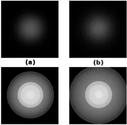
The kernel function used for splatting is usually based on the Normal distribution. However, we have found that this function is highly sensitive to changes in the visual param-eters. The ratio pixel-voxel in zooming views, the shading function used, the optical properties of the feature and the opacity required define the final size of the footprint to keep continuity between neighbor voxels. For instance, holes may appear when voxel’s opacity decreases, requiring changes in the footprint size. These effects are specially noticeable at the boundary between features in tagged volume visualiza-tions. We propose to use a Beta function as thegeneric foot-print function, which improves the rendering performance using smaller footprints and that is easier to tune under vi-sual changes.

The Beta-function lets controlling separately the open-ness, height and width of the curve. The general Beta-function isBeta(x,a,b) =xa(1−x)b, where the parameters

aandbcontrol the shape of the curve in range[0,1]. Hence, scaling the range and giving identical values toaandb, we can obtain the set of symmetric curves showed in Figure3. This figure shows that it is possible to force the curve’s width (i.e.[−5..5]) while controlling the curve’s shape: lowera,b

values produce curves more opened.

Beta(x,a,b) =kscalexa(1−x)b (1)

Figure 3:Beta D. with different exponent values.

Figure4shows that we can use a smaller footprint based on beta distribution to obtain a splat similar to a normal dis-tribution based footprint.

Image-aligned splatting slices the interpolation kernels by a series of cutting planes aligned parallel to image plane. The kernel sections share the same weight distribution but they have different radius depending on the cutting plane. We use a kernel base distribuiton and a scaling factor as [MC98] to

Figure 4:Splats: [top row] The 256 pixelsbeta-footprint(a) re-quires a26.8%smaller footprint than the 350 pixelsgauss-footprint

(b); [bottom row] The same images but filtered to highlight the val-ues even when they become close to zero. They reveal that the gauss-footprinthas more extension to fall to almost zero than the beta-footprint.

obtain them. Figure5shows a single kernel composed of seven stacked section footprints.

Figure 5:Stacked set of differentbeta-footprintscorresponding to a single kernel and a graph displaying the footprint’s weights along the central footprint.

In addition, an alpha-blend operator is used to compose the kernel sections that fall within the same sheet-bucket, in-stead the theaddoperator proposed in [MC98]. This alpha composition provides a smoother color transitions between overlapped kernel sections. Figure5illustrates the smooth interfaces between different optical properties and resolu-tions.

Figure 6:Interface of two resolutions: [left] six voxels at resolu-tion 1 (the first four in red color and the last two in cyan color) [right] one voxel at resolution 2 (red) and two voxels at resolution 1 (cyan).

6. Simulations

The proposedFeature Graphmodel has been tested with two real datasets. All the tests were run on an AMD 64 3200+ with 1MB of RAM and an NVidia GeForce 6600 256MB. The datasets are tagged volumes with different ma-terial properties for each label. They are tested on our soft-ware platformHipo[CPT06].

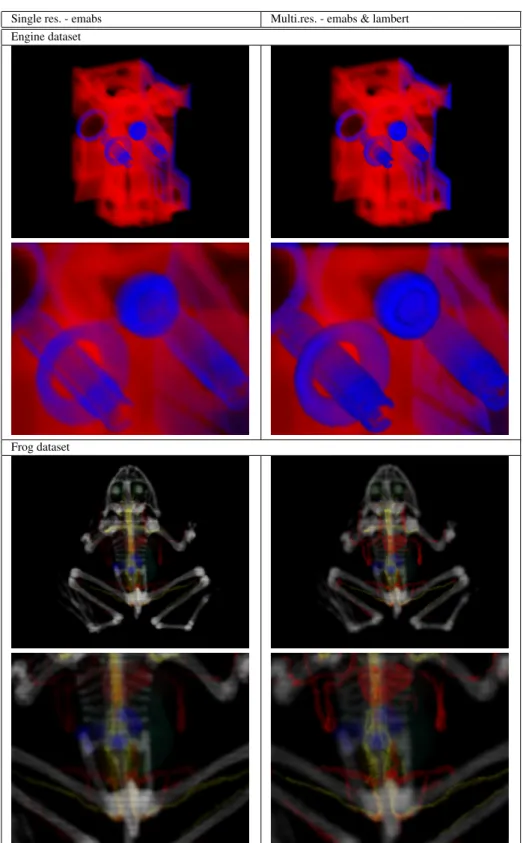
The resulting images of these simulations are placed in the Table 1. The first column shows the pictures of render-ing the Feature Graph with all the sets of voxels at a reso-lution of 2563using an emission+absorption shading model (emabs). In contrast, the second column shows renderings of the Feature Graph at different resolutions and different shading models according to a Focus+Context schema. The focus is rendered at the original 2563 resolution while the context is subsampled at coarser resolutions (up to 1283). Even more, the surface of what we focus on, is rendered us-ing a Lambert shadus-ing model while all the rest is rendered following theemabsmodel. Besides, the second row of each dataset contains a zoomed view of it.

The first model contains the classical engine block dataset, with a geometry of 256x256x152. The first col-umn shows thatbeta footprintsandαCompositionprovide smooth images with good visual quality even at zoomed views. The ratio pixels/voxel is 1.42 in the upper row, and 4.93 in the second row. In this case, the Feature Graph has been used to access directly to the voxels of the two selected features and render each one with different transfer func-tions. The last column shows how the Feature Graph can be used to obtain Focus+Context images. The focus -in blue color- is rendered using a Lambert shading model in its sur-face to enhance its edges, while the context -in red color- is rendered at a low resolution. The second dataset is the com-puter tomography of a frog, with a geometry of 256x236x72. In this case the ratio pixels/voxels of the first column is 1.74 in its upper row and 3.86 in the last row. The last column also has Focus+Context images where the focus is the ner-vous and venous systems and the rest of the frog body is the context environment.

Figure 7:Beta and Gauss footprints used with real datasets: the image rendered using 25x25 pixel beta footprints [left] has mainly the same appearance than the one rendered using 35x35 pixel gauss footprints [right], but requires half the time to be rendered.

Finally, Figure6shows a comparison of the engine block dataset rendered using the Beta footprints or the usual Nor-mal distribution based footprints. The visual quality is equiv-alent, although beta footprints are smaller. As a conse-quence, in the example, the execution is twice faster when using beta footprints.

7. Conclusions and future work

We have proposed to represent classified datasets as a fea-ture graph. Our data strucfea-ture represents each feafea-ture at its own convenient level of resolution. Moreover, it can handle multiresolution representation. We have shown how to ren-der the graph using a view-aligned splatting method. To do so, we have proposed a 2D kernel function for splats that is easy to tune and generates smaller footprints that reduce the render time.

Our graph can be extended in many ways. First, we want to explore how to render it with other algorithms than view-aligned splatting. Storing theSOV s of the features as 3D textures seems a promising way to render the model using hardware-driven texture mapping or ray-casting. In addition, we want to add other geometric models to the features, as for instance a polygonal model of the surfaces extracted in a pre-process. This way, we would be able to render some fea-tures as surfaces and other as volumes. Again, depth sorting problems and transition artifacts between the different geo-metrical model will need to be solved. Finally, we would like to assign levels of importance to the features, that combined with their degree of focus would provide better automatic means of selecting for each feature its convenient graphical model, resolution and optical properties.

References

[Ba05] BIRKFELLNERW.,AL.: Wobbled splatting: a fast perspective volume rendering method for simulation of x-ray images from ct. Physics in Medicine and Biology 50

(2005), 73–84.

for volume data.IEEE Trans. on Visualization and Com-puter Graphics 12, 5 (2006), 1077–1084.

[CPT06] CAMPOSJ., PUIG A., TOSTD.: Efficient fo-cus+context visual exploration of volume datasets. In

EG/ACM SIGGRAPH SIAGC’06(2006), pp. 79–88.

[CSW∗03] CHENM., SILVERD., WINTERA. S., SINGH V., CORNEAN.: Spatial transfer functions: a unified ap-proach to specifying deformation in volume modeling and animation. InVolume Graphics’03(2003), pp. 35–44. [DKC00] DONG F., KROKOS M., CLAPWORTHY G.:

Fast volume rendering and data classification using mul-tiresolution min-max octrees.Comput. Graph. Forum 19, 3 (2000).

[FPT06] FERRÉM., PUIG A., TOSTD.: Decision trees for accelerating unimodal, hybrid and multimodal render-ing models.The Visual Computer 3(2006), 158–167. [GDF03] GUTWINC., DYICKJ., FEDAKC.: The effects

of dynamic transparency on targeting performance isosur-faces. InGraphics Interface’03(2003), pp. 105–112. [HBH03] HADWIGER M., BERGER C., HAUSER H.:

High-quality two-level volume rendering of segmented data sets on consumer graphics Hardware. InIEEE Vi-sualization ’03(2003), pp. 40–45.

[HCS98] HUANGJ., CRAWFISR., STREDNEYD.: Edge preservation in volume rendering using splatting. InIEEE Visualization’98(1998), pp. 63–69.

[HMBG01] HAUSER H., MROZ L., BISCHI G., GRÖLLER M.: Two-level volume rendering. IEEE

Trans. on Visualization and Computer Graphics 7, 3

(2001), 242–252.

[KCOY03] KADOSHA., COHEN-ORD., YAGELR.: Vol-ume graphics. IEEE Trans. on Visualization and Com-puter Graphics 9, 4 (2003), 580–586.

[LH91] LAURD., HANRAHANP.: Hierarchical splatting: A progressive refinement algorithm for volume rendering.

ACM Computer Graphics 25, 4 (July 1991), 285–318.

[LMK03] LIW., MUELLERK., KAUFMAN A.: Empty space skipping and occlusion clipping for texture based volume rendering. InIEEE Visualization 2003(2003), pp. 317–324.

[MC98] MUELLERH., CRAWFIS R.: Eliminating pop-ping artifacts in sheet buffer-based splatting. IEEE Visu-alization’98(1998), 239–246.

[MLK03] MUELLER K., LAKARE S., KAUFMAN A.: Volume exploration made easy using feature maps. In

Workshop on Scientific Visualization(2003).

[MM01] MEREDITHJ., MAK.-L.: Multiresolution view-dependent splat based volume rendering of large irregular data. 2001 Symp. on Parallel and Large-Data Visualiza-tion and Graphics(Oct. 2001), 93–99, 155.

[MMC99] MUELLER K., MÖLLER T., CRAWFIS R.: Splatting without the blur. In IEEE Visualization’99

(1999), pp. 363–371.

[MMI∗98] MUELLER K., MÖLLER T., II J. E. S., CRAWFISR., SHAREEFN., YAGELR.: Splatting errors and antialiasing. IEEE Trans. on Visualization and Com-puter Graphics 4, 2 (1998), 178–191.

[Pa01] PFISTERH.,AL.: The transfer function bake-off.

IEEE Computer Graphics & Applications 21, 3 (2001), 16–22.

[PTN00] PUIGA., TOSTD., NAVAZO M. I.: A hybrid model for vascular tree structures. InData Visualization

(2000), pp. 125–135.

[SSC03] SINGH V., SILVER D., CORNEA N.: Real-time volume manipulation. InVolume Graphics(2003), pp. 45–52.

[TSH98] TIEDE U., SCHIEMANN T., HOHNE K. H.: High quality rendering of attributed volume data. Proc.

IEEE Visualization(1998), 255–262.

[VHN∗05] VEGA F., HASTREITER P., NARAGHI R., FAHLBUSCHR., GREINERG.: Smooth volume rendering of labeled medical data on consumer graphics hardware.

InProc. of SPIE Medical Imaging 2005(2005), pp. 13–

21.

[VKG05] VIOLA I., KANITSAR A., GRÖLLER M. E.: Importance-driven feature enhancement in volume visu-alization. IEEE Trans. on Visualization and Computer Graphics 11, 4 (2005), 408–418.

[vW05] VAN WIJKJ. J.: The value of visualization. In

IEEE Visualization’05(2005), IEEE Press, pp. 76–86. [Wes89] WESTOVER L.: Interactive volume rendering.

In Volume Visualization Workshop (1989), ACM Press,

pp. 9–16.

[WG94] WILHEMSJ., GELDERA. V.: Multidimensional trees for controlled volume rendering and compression.

ACM Symp. on Volume Visualization 11(Oct. 1994), 27–

34.

[WJ06] WALTONS. J., JONESM. W.: Volume wires: a framework for empirical non-linear deformation of volu-metric datasets.The Journal of WSCG 14(2006), 81–88. [ZPvBG01] ZWICKER M., PFISTER H.,VAN BAAR J.,

GROSS M.: EWA volume splatting. InIEEE Visualiza-tion’01(2001), pp. 29–36.

Single res. - emabs Multi.res. - emabs & lambert Engine dataset

Frog dataset