Bandit-Aided Boosting

Bandit-Aided Boosting

R. Busa-Fekete, B. K´

egl

To cite this version:

R. Busa-Fekete, B. K´

egl. Bandit-Aided Boosting. OPT 2009: 2nd NIPS Workshop on

Opti-mization for Machine Learning, Dec 2009, Whistler, Canada.

<

in2p3-00580588

>

HAL Id: in2p3-00580588

http://hal.in2p3.fr/in2p3-00580588

Submitted on 28 Mar 2011

HAL

is a multi-disciplinary open access

archive for the deposit and dissemination of

sci-entific research documents, whether they are

pub-lished or not.

The documents may come from

teaching and research institutions in France or

abroad, or from public or private research centers.

L’archive ouverte pluridisciplinaire

HAL

, est

destin´

ee au d´

epˆ

ot et `

a la diffusion de documents

scientifiques de niveau recherche, publi´

es ou non,

´

emanant des ´

etablissements d’enseignement et de

recherche fran¸

cais ou ´

etrangers, des laboratoires

publics ou priv´

es.

Bandit-Aided Boosting

R´obert Busa-Fekete∗, Bal´azs K´egl†

LAL/LRI, University of Paris-Sud, CNRS Orsay, 91898, France

{busarobi,kegl}@gmail.com

Abstract

In this paper we apply multi-armed bandits (MABs) to accelerate ADABOOST. ADABOOSTconstructs a strong classifier in a stepwise fashion by selecting sim-ple base classifiers and using their weighted “vote” to determine the final classi-fication. We model this stepwise base classifier selection as a sequential decision problem, and optimize it with MABs. Each arm represent a subset of the base classifier set. The MAB gradually learns the “utility” of the subsets, and selects one of the subsets in each iteration. ADABOOSTthen searches only this subset in-stead of optimizing the base classifier over the whole space. The reward is defined as a function of the accuracy of the base classifier. We investigate how the MAB algorithms (UCB, UCT) can be applied in the case of boosted stumps, trees, and products of base classifiers. On benchmark datasets, our bandit-based approach achieves only slightly worse test errors than the standard boosted learners for a computational cost that is an order of magnitude smaller than with standard AD

-ABOOST.

1

Introduction

ADABOOST [1] is one of the best off-the-shelf learning methods developed in the last decade. It constructs a classifier in a stepwise fashion by adding simple classifiers (called base classifiers) to a pool, and using their weighted “vote” to determine the final classification. The simplest base learner used in practice is the decision stump, a one-decision two-leaf decision tree. Learning a decision stump means to select a feature and a threshold, so the running time of ADABOOSTwith stumps is proportional to the number of data pointsn, the number of attributesd, and the number of boosting iterationsT. When trees [2] or products [3] are constructed over the set of stumps, the computational cost is multiplied by an additional factor of the number of tree levelsN or the number of termsm. Although the running time is linear in each of these factors, the algorithm can be prohibitively slow if the data sizenand/or the number of featuresdis large.

There are essentially two ways to accelerate ADABOOST in this setting: one can either limit the number of data pointsnused to train the base learners, or one can cut the search space by using only a subset of thedfeatures. Although both approaches increase the number of iterationsT needed for convergence, the net computational time can still be significantly decreased. The former approach has a basic version when the base learner is not trained on the whole weighted sample, rather on a small subset selected randomly using the weights as a discrete probability distribution [1]. A recently proposed algorithm of the same kind is FILTERBOOST[4], which assumes that an oracle can produce an unlimited number of labeled examples, one at a time. In each boosting iteration, the oracle generates sample points that the base learner can either accept or reject, and then the base learner is trained on a small set of accepted points. The latter approach was proposed by [5] which introduces several feature selection and ranking methods used to accelerate ADABOOST. In

∗

R´obert Busa-Fekete is on leave from Research Group on Artificial Intelligence of the Hungarian Academy of Sciences and University of Szeged, Hungary

†

particular, the LAZYBOOST algorithm chooses a fixed-size random subset of the features in each boosting iteration, and trains the base learner using only this subset.

In this paper we aim to improve the latter approach by “aiding” the random feature selection. It is intuitively clear that certain features are more important than others for classification. In specific applications the utility of features can be assessed a-priori (e.g., on images of characters, we know that background pixels close to the image borders are less informative than pixels in the middle of the images), however, our aim here is to learn the importance of features by evaluating their empirical performance during the boosting iterations. At the same time, in boosting it is important to keep a high level of base learner diversity, which is the reason why we opted for using multi-armed bandits (MAB) which are known to manage the exploration-exploitation trade-off very well.

MAB techniques have recently gained great visibility due to their successful applications in real life, for example, in the game of GO. In the classical bandit problem the decision maker can select an arm at each discrete time step [6]. Selecting an arm results in a random reward, and the goal of the decision maker is to maximize the expected sum of the rewards received. Our basic idea is to partition the base classifier space into subsets and use MABs to learn the utility of the subsets. In each iteration, the bandit algorithm selects an optimal subset, then the base learner finds the best base classifier in the subset and returns a reward based on the accuracy of this optimal base classifier. By reducing the search space of the base learner, we can expect a significant decrease of the complete running time of ADABOOST. case of decision stumps, we use the

The paper is organized as follows. First we describe the ADABOOST.MH algorithm and the neces-sary notations in Section 2. Section 3 contains our main contribution of using MABs for accelerating the selection of base classifiers. We present experimental results in Section 4, and conclude in Sec-tion 5.

2

A

B

.MH

For the formal description letX= (x1, . . . ,xn)be then×dobservation matrix, wherex (j)

i are

the elements of thed-dimensional observation vectorsxi ∈ Rd. We are also given a label matrix

Y = (y1, . . . ,yn)of dimensionn×Kwhereyi ∈ {+1,−1}K. In multi-class classification one

and only one of the elements ofyi is+1, whereas in multi-label (or multi-task) classificationyi

is arbitrary, meaning that the observationxi can belong to several classes at the same time. In the

former case we will denote the index of the correct class by`(xi).

The goal of the ADABOOST.MH algorithm ( [1]) is to return a vector-valued classifierf :X →_RK

with a small Hamming loss RH f(T)_,W(1)

= Pn i=1 PK `=1w (1) i,`I n sign f<sub>`</sub>(T)(xi) 6 =yi,`o1 _by

minimizing its upper bound (the exponential margin loss)

Re f(T),W(1) = n X i=1 K X `=1

w(1)_{i,`</sub> exp −f<sub>`}(T)(xi)yi,`

, (1)

wheref`(xi)is the`th element off(xi). ADABOOST.MH builds the final classifierf as a sum of

base classifiersh(t)_{: X →}

RK returned by a base learner algorithm BASE(X,Y,W(t))in each iterationt. In general, the base learner should seek to minimize the base objective

E h,W(t)= n X i=1 K X `=1

w<sub>i,`</sub>(t)exp −h`(xi)yi,`. (2)

Using the weight update formula of ADABOOST.MH, it can be shown that

Re f(T),W(1) = T Y t=1 E h(t),W(t) , (3)

so minimizing (2) in each iteration is equivalent to minimizing (1) in an iterative greedy fash-ion. By obtaining the multi-class prediction`(bx) = arg max`f

(T)

` (x),it can also be proven that

the “traditional” multi-class loss (or one-error)R f(T)

=Pn i=1I n `(xi)6=b`(xi) o has an upper boundKRe f(T),W(1)

if the weights are initialized uniformly, and√K−1Re f(T),W(1)

with a multi-class initialization. This justifies the minimization of (1).

1

2.1 Learning the base classifier

In this paper we use discrete ADABOOST.MH in which the vector-valued base classifierh(x)is represented ash(x) =αvϕ(x),whereα∈_R+_{is the base coefficient,v∈ {+1,−1}}K _{is the vote}

vector, andϕ(x) :Rd → {+1,−1}is a scalar base classifier. It can be shown that for minimizing

(2), one has to chooseφthat maximizes the edgeγ=Pn

i=1

PK

`=1wi,`v`ϕ(xi)yi,`,using the votes v`= <sub>1 if</sub> Pn i=1wi,`I{ϕ(xi) =yi,`}>P n i=1wi,`I{ϕ(xi)6=yi,`}, −1 otherwise, `= 1, . . . , K. (4)

It is also well known that the base objective (2) can be expressed as

E h,W

=p(1 +γ)(1−γ) =p1−γ2_{. (5)}

In our experiments we used three base learners: decision stumps, decision trees, and products of decision stumps. The technical details of their implementations can be found in [3].

3

Using multi-armed bandits to reduce the search space

In this section we will first describe the MAB framework and the two particular algorithms we use. The next subsection contains our main contribution: we show how bandit algorithms can be used to accelerate the base learning step in AdaBoost.

3.1 Multi-armed bandits

In the classical bandit problem there areM arms that the decision maker can select at discrete time steps. Selecting armj in iterationtresults in a random rewardr_j(t)∈[0,1]whose (unknown) dis-tribution depends onj. The goal of the decision maker is to maximize the expected sum of the rewards received. Intuitively, the decision maker’s policy has to balance between using arms with large past rewards (exploitation) and trying arms that have not been tested enough times (explo-ration). The UCB algorithm [6] manages this trade-off by choosing the arm that maximizes the sum of the average rewardr(_jt) = 1

T_j(t)

Pt

t0₌₁I{armjis selected}r

(t0)

j and a confidence interval term c(_jt) =

r

2 lnt

T_j(t),whereT

(t)

j is the number of times when armj has been selected up to iterationt.

To avoid the singularity atT_j(t)= 0, the algorithm starts by selecting each arm once. We also use a generalized version, denoted by UCB(k), in which the bestkarms are selected for evaluation, and the one that maximizes the actual rewardr(_jt)is finally chosen.

The UCT algorithm [7] is a tree search method based on UCB. It is used often when the number of arms is large. UCT organizes the arms into a rooted tree-structure where the leaves represent the arms. In each time step, UCT determines a path from the root to a leaf by greedily choosing each inner point that maximizes the upper confidence bound %(_jt) +

r

2 lnT_pj(t)

T_j(t) , wherepj is the

index of the parent of node j and%(_jt) is the average reward that has been obtained by all paths going through nodejselected up to iterationt. When the path is selected, the reward obtained by the leaf node is assigned to each inner point in the path. Initially, neither the average reward nor the confidence interval are available. Trying all arms (as in UCB) would be computationally very inefficient; instead we use random rewards and confidence intervals for previously unvisited nodes.

3.2 The application of bandit-based methods for accelerating AdaBoost

The general idea is to partition the base classifier space into (not necessarily disjunct) subsets and use MABs to learn the utility of the subsets. In each iteration, the bandit algorithm selects an optimal subset (or, in the case of UCB(k), a union of subsets). The base learner then finds the best base classifier in the subset, and returns a reward based on this optimal base learner. By reducing the search space of the base learner, we can expect a significant decrease of the complete running time of ADABOOST.

The upper bound (3) together with (5) suggest the use of−1

2log(1−γ

2_{)for the reward. In practice}

we found thatr(_jt) = 1−p1−γ2 _{works as well as the logarithmic reward; it was not surprising}

since the two are almost identical in the lower range of the[0,1]interval where the majority of the edges are. The latter choice has another advantage of always being in the[0,1]interval which is a formal requirement in MABs.

The actual partitioning of the base classifier set depends on the particular base learner. In the case of decision stumps, the most natural choice for UCB is to assign each feature to a subset. In principle, we could also further partition the threshold space but that would not lead to further savings in the linear computational time since, because of the changing weightswi,`, all data points and labels would have to be visited anyway. On the other hand, subsets that contain more than one feature can be efficiently handled by UCB(k).

In the case of trees and products we have more choices. We use UCB by considering each tree or product as a sequence of decisions, and using the same partitioning as with decision stumps at each inner node. In this setup we lose the information in the dependence of the decisions on each other

within a tree or a product. A more natural choice for these base learners is to use UCT. In this

solution we can consider each base classifier as a sequence, and use the tree-structured bandit for partitioning the (very large) sequence space. The partitioning follows naturally the sequence defined by the classification tree itself. The setup works also for products: even though the commutative product would suggest to represent subsets by arms, the greediness of the learning algorithm de-scribed in [3] makes sequences a more natural choice. Note that, in the case of trees, both (UCB and UCT) setups reduce the actual search space by construction since brothers having the same parent must act on the same feature (or one of a few number of features in UCB(k)) whereas, in general, brothers are independent.

4

Experiments

To test the algorithms, we carried out experiments on a synthetic set and five benchmark datasets us-ing the standard train/test cuts2. Beside MAB-based ADABOOST(UCB(k)and UCT), we used two baselines: standard ADABOOST.MH with full search (FULL), and ADABOOST.MH with searching only a random subset ofkfeatures each time a decision stump is required (RANDOM(k)), that is, in each iteration when using decision stumps, and at each level when using trees or products. Instead of validatingT and performing an early stopping, we decided to run the algorithm for a long time (T = 105in each experiment), and measure the average of th test error (2) on the lastT /5iterations to obtainR f(T) = 5 T PT t=4T /5R f (t)

. The advantage of this approach is that this estimate is more robust in terms of random fluctuations after convergence than the raw errorR f(T)

at a given iteration. It is also a pessimistic estimate of the error when there is a slight over- or underfitting (since the average is always an upper bound of the minimum) which was rarely observed on these sets. The hyperparametersN andmwere selected by80%-20% simple validation on the training set using full ADABOOST.MH.

The first experiment was a simple test to validate the hypothesis that MABs may help ADABOOST

to find “useful” features. We generated a10-dimensional two-class data set in which only one of the features contained information about the labels3. As expected, full ADABOOST.MH (with decision stumps) used almost all the time the useful feature, whereas RANDOM(1)and RANDOM(3)used it in only10% and30% of the iterations, respectively. On the other hand, UCB(1)and UCB(3)found the good feature in17.5% and90% of the iterations, respectively.

Table 1 shows the asymptotic test errors on the benchmark datasets after105_{iterations. The first}

observation is that full ADABOOST.MH wins most of the times although the differences are rather small. The few cases where RANDOMor UCB/UCT beats full ADABOOST.MH could be explained by statistical fluctuations or the regularization effect of randomization. Secondly, UCB/UCT seems slightly better than RANDOMalthough the differences are even smaller. The difference seems more significant on the MNIST set where the number of features is rather large and some of the features are known to be useless.

Our main goal was not to beat full ADABOOST.MH in test performance, but to improve its compu-tational complexity. So we were not so much interested in the asymptotic test errors but rather the speed by which acceptable test errors are reached. As databases become larger, it is not unimagin-able that certain algorithms cannot be run with their statistically optimal hyperparameters (T in our case) because of computational limits, so managing underfitting (an algorithmic problem) is more important than managing overfitting (a statistical problem) [8]. To illustrate how the algorithms

be-2

The data sets (selected based on their wide usage and their large sizes) are available at

yann.lecun.com/exdb/mnist (MNIST), www.kernel-machines.org/data.html (USPS),

andwww.ics.uci.edu/˜mlearn/MLRepository.html(letter, pendigit, isolet).

3_x(j)

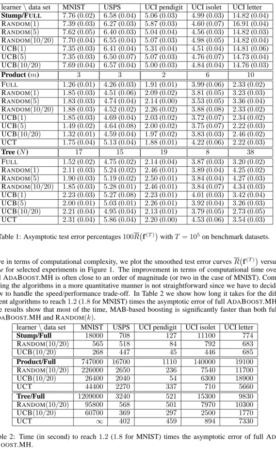
learner\data set MNIST USPS UCI pendigit UCI isolet UCI letter Stump/FULL 7.76(0.02) 6.58(0.04) 5.06(0.03) 4.99(0.03) 14.82(0.04) RANDOM(1) 7.39(0.03) 6.27(0.03) 5.87(0.03) 4.60(0.07) 16.91(0.04) RANDOM(5) 7.62(0.05) 6.40(0.03) 5.04(0.04) 4.56(0.03) 14.82(0.03) RANDOM(10/20) 7.70(0.04) 6.55(0.04) 5.07(0.03) 4.98(0.05) 14.82(0.04) UCB(1) 7.35(0.03) 6.41(0.04) 5.31(0.04) 4.51(0.04) 14.81(0.06) UCB(5) 7.35(0.03) 6.50(0.07) 5.07(0.03) 4.76(0.07) 14.73(0.04) UCB(10/20) 7.69(0.04) 6.57(0.04) 5.00(0.03) 4.84(0.04) 14.76(0.03) Product (m) 3 3 2 6 10 FULL 1.26(0.01) 4.26(0.03) 1.91(0.01) 3.99(0.06) 2.33(0.02) RANDOM(1) 1.85(0.03) 4.51(0.06) 2.09(0.02) 3.81(0.05) 3.23(0.03) RANDOM(5) 1.83(0.03) 4.74(0.04) 2.14(0.00) 3.53(0.05) 3.36(0.04) RANDOM(10/20) 1.88(0.03) 4.52(0.02) 2.26(0.02) 3.88(0.08) 2.33(0.02) UCB(1) 1.85(0.03) 4.69(0.04) 2.03(0.02) 3.72(0.07) 2.34(0.02) UCB(5) 1.49(0.02) 4.64(0.08) 2.00(0.02) 3.75(0.07) 2.22(0.03) UCB(10/20) 1.32(0.01) 4.59(0.04) 1.97(0.02) 3.83(0.03) 2.46(0.02) UCT 1.75(0.04) 5.13(0.04) 1.88(0.01) 4.22(0.06) 2.22(0.03) Tree (N) 17 15 19 8 38 FULL 1.52(0.02) 4.75(0.02) 2.14(0.04) 3.87(0.03) 3.20(0.02) RANDOM(1) 2.11(0.03) 5.24(0.02) 2.46(0.01) 3.89(0.04) 4.25(0.02) RANDOM(5) 1.90(0.03) 5.19(0.02) 2.50(0.01) 3.84(0.04) 4.27(0.03) RANDOM(10/20) 1.85(0.03) 5.28(0.01) 2.46(0.01) 3.84(0.07) 4.34(0.03) UCB(1) 2.23(0.03) 5.27(0.08) 2.23(0.01) 4.01(0.03) 3.42(0.04) UCB(5) 2.00(0.01) 5.03(0.01) 2.26(0.01) 3.92(0.04) 3.26(0.03) UCB(10/20) 2.21(0.04) 4.95(0.04) 2.13(0.01) 3.79(0.05) 2.73(0.05) UCT 2.31(0.04) 5.86(0.04) 2.20(0.00) 4.53(0.06) 3.54(0.03) Table 1: Asymptotic test error percentages100R f(T)withT = 105on benchmark datasets.

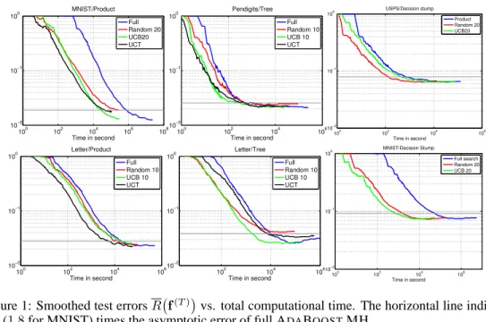
have in terms of computational complexity, we plot the smoothed test error curvesR f(T)

versus

time for selected experiments in Figure 1. The improvement in terms of computational time over

full ADABOOST.MH is often close to an order of magnitude (or two in the case of MNIST). Com-paring the algorithms in a more quantitative manner is not straightforward since we have to decide how to handle the speed/performance trade-off. In Table 2 we show how long it takes for the dif-ferent algorithms to reach1.2(1.8for MNIST) times the asymptotic error of full ADABOOST.MH. The results show that most of the time, MAB-based boosting is significantly faster than both full ADABOOST.MH and RANDOM(k).

learner\data set MNIST USPS UCI pendigit UCI isolet UCI letter

Stump/Full 18000 708 127 11100 774 RANDOM(10/20) 565 518 84 792 683 UCB(10/20) 268 447 45 446 685 Product/Full 747000 16700 1110 140000 19100 RANDOM(10/20) 226000 2650 236 7540 11700 UCB(10/20) 26400 2040 54 6300 18900 UCT 44400 2270 337 710 5660 Tree/Full 1209000 3240 521 15300 9830 RANDOM(10/20) 95800 568 501 7970 10300 UCB(10/20) 60700 369 297 2500 1770 UCT ∞ 402 459 894 7330

Table 2: Time (in second) to reach 1.2 (1.8 for MNIST) times the asymptotic error of full AD

-ABOOST.MH.

5

Conclusion

In this paper we asked a simple question: can ADABOOSTbe accelerated by modeling it as a sequen-tial decision problem, and optimizing it within this framework? To answer, we chose a particular

100 ₁₀2 ₁₀4 ₁₀6 ₁₀8 10−2 10−1 100 Time in second MNIST/Product Full Random 20 UCB20 UCT 100 ₁₀2 ₁₀4 ₁₀6 10−2 10−1 100 Time in second Pendigits/Tree Full Random 10 UCB 10 UCT 100 ₁₀2 ₁₀4 ₁₀6 10−2 10−1 100 Time in second USPS/Decision stump Product Random 20 UCB20 100 ₁₀2 ₁₀4 ₁₀6 10−2 10−1 100 Time in second Letter/Product Full Random 10 UCB 10 UCT 102 ₁₀4 ₁₀6 10−2 10−1 100 Time in second Letter/Tree Full Random 10 UCB 10 UCT 100 ₁₀2 ₁₀4 ₁₀6 10−2 10−1 100 Time in second MNIST/Decision Stump Full search Random 20 UCB 20

Figure 1: Smoothed test errorsR f(T)

vs. total computational time. The horizontal line indicates

1.2(1.8for MNIST) times the asymptotic error of full ADABOOST.MH.

setup (multi-armed bandits), and made several modeling and algorithmic choices within the frame-work. Since our goal was to improve the speed of ADABOOST, most of our choices are justified by arguments of algorithmic simplicity and computational complexity. On the other hand, to keep the project within manageable limits, we consciously did not explore all the possible avenues. For example, multi-armed bandits assume a stateless system, whereas ADABOOSThas a natural state descriptor: the weight matrixW(t). In this setup a Markov decision process would be more natural choice.

Our answer to the original question is two-fold: it seems that the asymptotic test error of ADABOOST

with full search is hard to beat, so if we have enough computational resources to reach the flattening of the test error curve, we should use full ADABOOST. On the other hand, in large scale learning (recently publicized in a seminal paper by Bottou and Bousquet [8]), where we stay in an underfitting regime and so fast optimization becomes more important than asymptotic statistical optimality, our MAB-optimized ADABOOSTcan find its niche.

References

[1] Y. Freund and R. E. Schapire. A decision-theoretic generalization of on-line learning and an application to boosting. Journal of Computer and System Sciences, 55:119–139, 1997.

[2] J. Quinlan. C4.5: Programs for Machine Learning. Morgan Kaufmann, 1993.

[3] B. K´egl and R. Busa-Fekete. Boosting products of base classifiers. In Proceedings of the 26th

International Conference on Machine Learning, 2009.

[4] J.K. Bradley and R.E. Schapire. FilterBoost: Regression and classification on large datasets. In

Advances in Neural Information Processing Systems, volume 20, pages 185–192, 2008.

[5] G. Escudero, L. M`arquez, and G. Rigau. Boosting applied to word sense disambiguation. In

Proceedings of the 11th European Conference on Machine Learning, pages 129–141, 2000.

[6] P. Auer, N. Cesa-Bianchi, and P. Fischer. Finite-time analysis of the multiarmed bandit problem.

Machine Learning, 47:235–256, 2002.

[7] L. Kocsis and Cs. Szepesv´ari. Bandit based Monte-Carlo planning. In Proceedings of the 17th

European Conference on Machine Learning, pages 282–293, 2006.

[8] L. Bottou and O. Bousquet. The tradeoffs of large scale learning. In Advances in Neural