A Dissertation by
RAJESH TALLURI
Submitted to the Office of Graduate Studies of Texas A&M University
in partial fulfillment of the requirements for the degree of DOCTOR OF PHILOSOPHY
August 2011
A Dissertation by
RAJESH TALLURI
Submitted to the Office of Graduate Studies of Texas A&M University
in partial fulfillment of the requirements for the degree of DOCTOR OF PHILOSOPHY
Approved by:
Co-Chairs of Committee, Bani K. Mallick
Veerabhadran Baladandayuthapani Committee Members, Jeffrey D. Hart
Aniruddha Datta Head of Department, Simon J. Sheather
August 2011
ABSTRACT
Bayesian Gaussian Graphical Models Using Sparse Selection Priors and Their Mixtures. (August 2011)
Rajesh Talluri, B.Tech., Indian Institute of Technology, Guwahati Co-Chairs of Advisory Committee: Dr. Bani K. Mallick
Dr. Veerabhadran Baladandayuthapani
We propose Bayesian methods for estimating the precision matrix in Gaussian graphical models. The methods lead to sparse and adaptively shrunk estimators of the precision matrix, and thus conduct model selection and estimation simultaneously. Our methods are based on selection and shrinkage priors leading to parsimonious parameterization of the precision (inverse covariance) matrix, which is essential in several applications in learning relationships among the variables. In Chapter I, we employ the Laplace prior on the off-diagonal element of the precision matrix, which is similar to the lasso model in a regression context. This type of prior encourages sparsity while providing shrinkage estimates. Secondly we introduce a novel type of selection prior that develops a sparse structure of the precision matrix by making most of the elements exactly zero, ensuring positive-definiteness.
In Chapter II we extend the above methods to perform classification. Reverse-phase protein array (RPPA) analysis is a powerful, relatively new platform that allows for high-throughput, quantitative analysis of protein networks. One of the challenges that currently limits the potential of this technology is the lack of methods that allows for accurate data modeling and identification of related networks and samples. Such models may improve the accuracy of biological sample classification based on patterns of protein network activation, and provide insight into the distinct biological relationships underlying different cancers. We propose a Bayesian sparse graphical modeling
approach motivated by RPPA data using selection priors on the conditional relationships in the presence of class information. We apply our methodology to an RPPA data set generated from panels of human breast cancer and ovarian cancer cell lines. We demonstrate that the model is able to distinguish the different cancer cell types more accurately than several existing models and to identify differential regulation of components of a critical signaling network (the PI3K-AKT pathway) between these cancers. This approach represents a powerful new tool that can be used to improve our understanding of protein networks in cancer.
In Chapter III we extend these methods to mixtures of Gaussian graphical models for clustered data, with each mixture component being assumed Gaussian with an adaptive covariance structure. We model the data using Dirichlet processes and finite mixture models and discuss appropriate posterior simulation schemes to implement posterior inference in the proposed models, including the evaluation of normalizing constants that are functions of parameters of interest which are a result of the restrictions on the correlation matrix. We evaluate the operating characteristics of our method via simulations, as well as discuss examples based on several real data sets.
ACKNOWLEDGMENTS
It was a treatise to work with Dr. Bani Mallick as he has an uncanny ability to envision cutting-edge problems. As a result, I got an opportunity to work on problems of practical significance with applications in diverse areas. His wisdom on conducting research and research management has surely benefited my research. I consider myself extremely fortunate to have worked under his supervision, and his pleasant personality always made the work environment a home away from home.
My collaboration with Dr. Veera started with a summer internship. During our time together, his style of functioning, his way of translating ideas into algorithms, his planning and scheduling of work and his views of using statistics from application point of view have greatly influenced my work. I thank him for being on my dissertation committee.
Any graduate student in the department agrees in no uncertain terms, that Dr. Mike Longnecker is a role model for any aspiring teacher. He corrected me whenever I was off track and made me realize how serious graduate education is in the US. I thank my lab mate Soma, for inspiring some new ideas and making my grad life filled with fun.
TABLE OF CONTENTS
CHAPTER Page
I INTRODUCTION TO BAYESIAN ADAPTIVE GAUSSIAN
GRAPH-ICAL MODELS . . . . 1
A. Introduction . . . 1
B. The Bayesian Lasso Model for Sparse Graphical Models . . . . 5
1. Posterior inference and conditionals for the Bayesian Lasso Model . . . 7
2. Posterior thresholding for sparse solutions in Bayesian Lasso Models . . . 10
C. The Bayesian Lasso Selection Model for Sparse Graphical Models . . . 12
1. Modelling the shrinkage matrixR . . . 12
2. Modelling the selection matrixA . . . 13
3. Conditional distributions and the posterior sampling for the selection model . . . 15
4. Model selection using marginal probabilities . . . 18
D. A Naive Bayesian Model . . . 20
E. Simulations . . . 21
F. Model Comparison with Benchmark Data . . . 29
1. Examples . . . 30
a. Example 1: Cork borings data set . . . 30
b. Example 2: The mathematics marks data set . . . 31
c. Example 3: Enron stock market data example . . . . 32
II BAYESIAN SPARSE GRAPHICAL MODELS FOR CLASSI-FICATION WITH APPLICATION TO PROTEIN EXPRESSION DATA . . . . 37
A. Introduction . . . 37
1. Protein signaling pathways in cancer . . . 37
2. Graphical models for network analysis . . . 39
B. Model . . . 41
1. Bayesian Sparse Gaussian Graphical Model with se-lection priors . . . 41
b. Incorporating prior pathway information . . . 46
2. Conditionals . . . 48
3. Bayesian classification based on posterior predictive probabilities . . . 50
C. Estimation Via MCMC . . . 52
D. FDR-based Determination of Significant Networks . . . 53
1. Application of the methodology to reverse-phase pro-tein lysate arrays . . . 55
E. Data Analysis . . . 59
1. Classification of breast and ovarian cancer cell lines . . . . 60
2. Effects of tissue culture conditions on network topology . . 65
F. Discussion and Conclusions . . . 71
III MIXTURES OF GAUSSIAN GRAPHICAL MODELS . . . . 73
A. Finite Mixtures of Gaussian Graphical Models . . . 73
1. Introduction . . . 73
2. The hierarchical model . . . 73
3. Posterior inference and the conditional distributions . . . . 75
4. Real data example . . . 78
5. Simulations . . . 81
B. Infinite Mixtures of Graphical Models . . . 86
1. Sampling fromHφ . . . 88
2. Real data example . . . 89
3. Simulations . . . 91
C. Discussion and Conclusions . . . 92
APPENDIX A . . . . 107
APPENDIX B . . . . 108
LIST OF TABLES
TABLE Page
I Predictive squared error comparison for Enron stock data . . . . 35 II Misclassification error rates for different classifiers for ovarian and
breast cancer data sets. The methods compared here are LDA (linear discriminant analysis), KNN (K-nearest neighbor), DQDA (diagonal quadratic discriminant analysis), DLDA (diagonal linear discriminant analysis) and BGBC (Bayesian graph-based classifier), which is the method studied in this paper. The mean and the standard deviation are values of the percentage misclassification over 100 random splits
LIST OF FIGURES
FIGURE Page
1 Shows the kernel density estimate of the empirical distributions of the
MCMC samples of the correlations. . . . . 11 2 This figure shows the simulated matrices for different types of
struc-tures for precision matrix. The colorbar is same for all the matrices. White indicates a zero in the precision matrix whereas colored cells
indicate non-zero elements. . . . . 22 3 This figure shows the comparison between 4 methods “glasso” -Friedman
et al. (2008), “MB”- Meinshausen and B´uhlmann (2006), “Bayesian lasso” model and “Bayesian lasso selection” model in terms of Kullback-Leibler loss (K-L) for the simulated simulated matrices for different
types of structures for precision matrix forp= 25. Lower is better. . . . . 26 4 This figure shows the comparison between 4 methods “glasso” -Friedman
et al. (2008), “MB”- Meinshausen and B´uhlmann (2006), “Bayesian lasso” model and “Bayesian lasso selection” model in terms of false positive rates for the simulated simulated matrices for different types
of structures for precision matrix forp= 25. Lower is better. . . . . 27 5 This figure shows the comparison between 4 methods “glasso” -Friedman
et al. (2008), “MB”- Meinshausen and B´uhlmann (2006), “Bayesian lasso” model and “Bayesian lasso selection” model in terms of false negative rates for the simulated simulated matrices for different types
of structures for precision matrix forp= 25. Lower is better. . . . . 28 6 (A) was selected by Lasso, Garrote and Naive Bayes Models and (B)
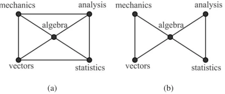
was selected by Bayesian lasso, Bayesian lasso selection and MIM Models. 30 7 (A) was selected by the Lasso model and (B) was selected by Bayesian
lasso, Bayesian lasso selection, MIM, garrote and Naive Bayes Models. . 31 8 This figure shows the top 6 graphical models for the stock market data,
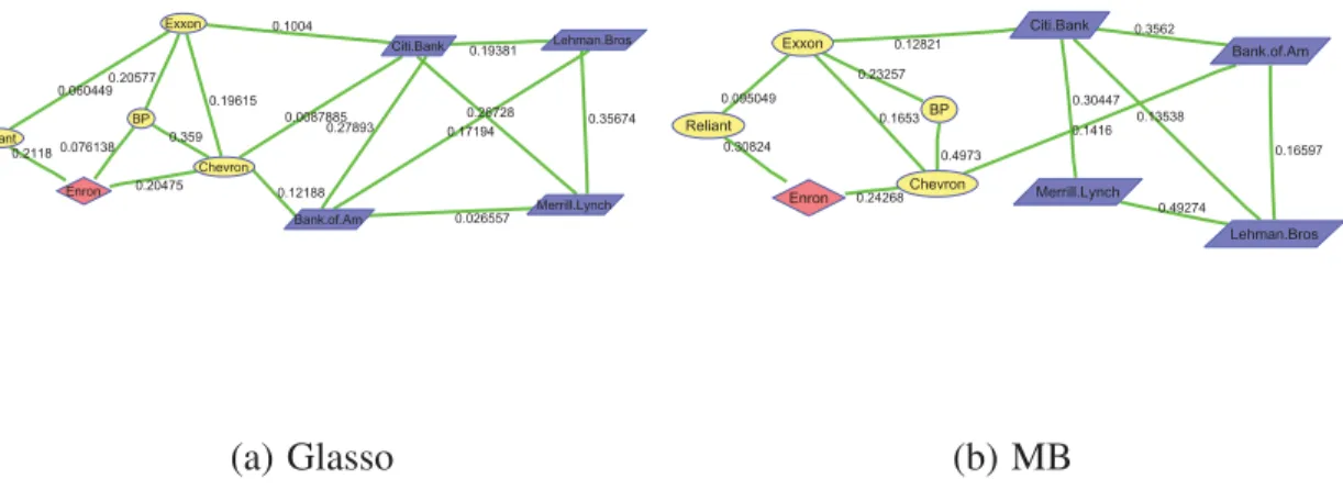
9 The graphical models for the stock market data obtained using (a) the
glasso method and (b) the MB method. . . . . 36 10 This figure shows the how the prior information is incorporated in
the model.qij is the model parameter which is the probability of there being an edge between protein i and protein j . If no information is available , prior on qij is Beta(2,2) with mean 0.5, reflecting no prior information about the edge and the prior on qij is Beta(10,2) with mean 0.83, if there is biological evidence that the edge plays an
important role in the pathway. . . . . 47 11 An example of a reverse-phase protein array (RPPA) slide with 40
samples shown as the 40 batches on the slide. Each batch represents one individual sample with 16 spots, which are the results of
dupli-cates of 8-step dilutions. . . . . 57 12 The PI3K-AKT Signaling Pathway. The pathway was generated through
the use of Ingenuity Pathways Analysis (www.ingenuity.com). . . . . 59 13 Significant edges for the proteins in the PI3K-AKT kinase pathway
for breast (left panel) and ovarian cancer cell lines (right panel) com-puted using Bayesian FDR of 0.10. The red (green) lines between the proteins indicate a negative (positive) correlation between the pro-teins. The thickness of the edges corresponds to the strength of the
associations, with stronger associations having greater thickness. . . . . 60 14 Conserved and differential networks for the proteins in the PI3K-AKT
kinase pathway between breast and ovarian cancer cell lines computed using Bayesian FDR set to 0.10. In the conserved network (top panel), the red (green) lines between the proteins indicate a negative (positive) correlation between the proteins. In the differential network (bottom panel) the blue lines between the proteins indicate a relationship sig-nificant in ovarian cell lines that was not sigsig-nificant in the breast cell lines; the orange lines between the proteins indicate a significant rela-tionship in the breast cell lines that was not significant in the ovarian cell lines. The thickness of the edges corresponds to the strength of
15 Nonlinear classification boundaries for two randomly selected covari-ates. Green points represent breast data and red points represent ovar-ian data. The blue line is the classification boundary determined by
the model, which tries to differentiate between breast and ovarian data. . . 66 16 Significant edges for the proteins in the PI3K-AKT kinase pathway
for ovarian cell lines grown in three different tissue culture condi-tions: A, B and C (see main text) computed using Bayesian FDR set to 0.10. The red (green) lines between the proteins indicate a nega-tive (posinega-tive) correlation between the proteins. The thickness of the edges corresponds to the strength of the associations, with stronger
associations having greater thickness. . . . . 68 17 Conserved and differential networks for the proteins in the PI3K-AKT
kinase pathway between ovarian cell lines grown in three different tis-sue culture conditions: A, B and C computed using Bayesian FDR set to 0.10. In the conserved network , the red (green) lines between the proteins indicate a negative (positive) correlation between the pro-teins. In the differential network, the blue lines between the proteins indicate a relationship significant in ovarian cell lines that was not sig-nificant in the breast cell lines; the orange lines between the proteins indicate a significant relationship in the breast cell lines that was not in the ovarian cell lines. The thickness of the edges corresponds to the strength of the associations, with stronger associations having greater
thickness. . . . . 69 18 Heat map of top 50 genes in leukaemia data set.. . . . 80 19 Significant edges for the genes in the ALL cluster. The red (green)
lines between the proteins indicate a negative (positive) correlation
between the proteins. . . . . 80 20 Significant edges for the genes in the AML cluster. The red (green)
lines between the proteins indicate a negative (positive) correlation
21 Simulation study (p=50). The true and estimated precision matrices for two subtypes of leukaemia: (a) ALL and (b) AML. The top row of images shows the true data generating precision matrix; the middle row shows the estimated precision matrix using our adaptive Bayesian model; and the bottom row shows the estimated precision matrix us-ing a non-adaptive fit. Note that the absolute values of the partial correlations are plotted in the above figures without the diagonal. The
colorbars are shown to the right of each image. . . . . 82 22 Simulation study(p=100). True and estimated precision matrices for
two subtypes of leukaemia: (a) ALL and (b) AML. The top row of images shows the true data generating precision matrix; the middle row shows the estimated precision matrix using our adaptive Bayesian model; and the bottom row shows the estimated precision matrix us-ing a non-adaptive fit. Note that the absolute values of the partial correlations are plotted in the above figures without the diagonal. The
colorbars are shown to the right of each image. . . . . 85 23 Graph for ALL Group.. . . . 90 24 Graph for AML Group. . . . . 91
CHAPTER I
INTRODUCTION TO BAYESIAN ADAPTIVE GAUSSIAN GRAPHICAL MODELS A. Introduction
Consider thepdimensional random vector Y = (Y(1),· · · , Y(p)), which follows a multi-variate normal distributionNp(μ,Σ)where both the meanμand the variance-covariance matrixΣare unknown. Flexible modelling of the covariance matrix,Σ, or equivalently the precision matrix,Ω=Σ−1, is one of the most important tasks in analysing Gaussian mul-tivariate data. Furthermore, it has a direct relationship to constructing Gaussian graphical models (GGMs) by identifying the significant edges. Of particular interest in this structure is the identification of zero entries in the precision matrixΩ. An off-diagonal zero entry
Ωij = 0 indicates conditional independence between the two random variables Y(i) and Y(j), given all other variables. This is the covariance selection problem or the model selec-tion problem in the Gaussian graphical models (Dempster, 1972; Speed and Kiiveri, 1986; Wong et al., 2003; Yuan and Lin, 2007), which provides a framework for the exploration of multivariate dependence patterns.
GGMs are tools for modelling conditional independence relationships. Among the practical advantages of using GGMs in high-dimensional problems is their ability to (i) make computations more efficient by alleviating the need to handle large matrices, (ii) yield better predictions by fitting sparser models, and (iii) aid scientific understanding by breaking down a global model into a collection of local models that are easier to search. Estimating the precision matrix efficiently and understanding its graphical structure is chal-lenging, however, due to a variety of reasons that we discuss hereafter.
A GGM for a random vector Y can be represented by an undirected graph G =
(V,E), where V containsp vertices corresponding to thepvariates and the edgesE =
(eij)(1≤i<j≤p) describe the conditional independence relationships among Y(1), . . . , Y(p). The edge betweenY(i)andY(j)is absent if and only ifY(i)andY(j)are independent, con-ditional on the other variables, which corresponds toΩij = 0. Thus, parameter estimation and model selection in the Gaussian graphical model are equivalent to estimating param-eters and identifying zeros in the precision matrix. The two main difficulties are that the number of unknown elements in the covariance matrix increases quadratically withp, and that it is difficult to deal directly with individual elements of the covariance matrix because it is necessary to keep the estimated matrix positive definite. Yang and Berger (1994) and Dempster (1969) pointed out that estimators based on scalar multiples of the sample co-variance matrix tend to distort the eigenstructure of the true coco-variance matrix unlessp/n is small. In this paper, we address these modelling and inferential challenges as we explore methods to adaptively estimate the precision matrix in a Gaussian graphical model setting. There have been many approaches to Gaussian graphical modelling. In a Bayesian setting, modelling is based on hierarchical specifications for the covariance matrix (or pre-cision matrix) using global priors on the space of positive-definite matrices, such as an inverse Wishart prior or its equivalents. Dawid and Lauritzen (1993) introduced an equiva-lent form as the hyper-inverse Wishart distribution. Although that construction enjoys many advantages, such as computational efficiency due to its conjugate formulation and exact cal-culation of marginal likelihoods (Scott and Carvalho, 2008), it is sometimes inflexible due to its restrictive form. Unrestricted graphical model determination is challenging unless the search space is restricted to decomposable graphs, where the marginal likelihoods are avail-able up to the overall normalizing constants (Giudici, 1996; Roverato, 2000). The marginal likelihoods are used to calculate the posterior probability of each graph, which gives an ex-act solution for small datasets, but a prohibitively large number of graphs for a moderately largep. Moreover, extension to a nondecomposable graph is nontrivial and
computation-ally expensive using reversible-jump algorithms (Giudici and Green, 1999; Brooks et al., 2003). There have been several attempts to shrink the covariance/precision matrix via matrix factorizations for unrestricted search over the space of both decomposable and non-decomposable graphs. Barnard et al. (2000) factorized the covariance matrix in terms of standard deviations and correlations, proposed several shrinkage estimators and discussed suitable priors. Wong et al. (2003) expressed the inverse covariance matrix as a product of the inverse partial variances and the matrix of partial correlations, then used reversible-jump-based Markov chain Monte Carlo (MCMC) algorithms to identify the zeros among the diagonal elements. Liechty et al. (2004) proposed flexible modelling schemes using decompositions of the correlation matrix.
Alternate approaches for more adaptive estimation and/or selection of the graphical models are based on priors/penalties that enforce sparsity. In a regression context for vari-able selection problems such priors have been proposed by George and McCulloch (1993, 1997); Kuo and Mallick (1998); Dellaportas et al. (2000, 2002). However the context of covariance selection in graphical models is inherently a different problem with additional complexity arising due to the additional constraints of positive definiteness and the num-ber of parameters to estimate being on the the order of p2 instead ofp. An alternate class of penalties that have received considerable attention in recent times have been lasso-type penalties (Tibshirani (1996)) that have the ability to promote sparseness, and have been used for variable selection in regression problems. In a frequentist graphical model context, Meinshausen and B´uhlmann (2006), Yuan and Lin (2007) and Friedman et al. (2008) pro-posed methods to estimate the precision or covariance matrix based on lasso-type penalties that yield only point estimates of the precision matrix. Lasso-based penalties are equivalent to Laplace priors in a Bayesian setting (Figueiredo, 2003; Bae and Mallick, 2004; Park and Casella, 2008). However, in a Bayesian setting, lasso penalties do not produce absolute zeros as the estimates of the precision matrix, and thus cannot be used to conduct model
selection simultaneously in such settings.
In this paper, we propose novel Bayesian methods for GGMs that allow for simul-taneous model selection and parameter estimation. We introduce a novel type of prior in Subsection C that can be decomposed into selection and shrinkage components in which lasso-type priors are used to accomplish shrinkage and variable selection priors are used for selection. We allow for local exploration of graphical dependencies that leads to a sparse structure of the precision matrix by enforcing most of the non-required elements to be ex-actly zero with positive probability while ensuring the estimate of the precision matrix is positive definite. More importantly, as a significant methodological innovation, we extend these methods to mixtures of GGMs for clustered data, with each mixture component as-sumed to be Gaussian with an adaptive covariance structure. For some kinds of data, it is reasonable to assume that the variables can be clustered or grouped based on sharing sim-ilar connectivity or graphs. Our motivation for this model arises from a high-throughput gene expression data set, for which it is of interest not only to cluster the patients (samples) into the correct subtype of cancer but also to learn about the underlying characteristics of the cancer subtypes. Of interest is differentiating the structure of the gene networks in the cancer subtypes as a means of identifying biologically significant differences that explain the variations between the subtypes. The modelling and inferential challenges are related to determining the number of components, as well as estimating the underlying graph for each component. We present a hierarchical extension of our adaptive methods for such settings, which, to the best of our knowledge, has not been addressed previously in the literature.
In this chapter, we propose novel Bayesian methods using shrinkage and selection priors for Gaussian graphical models that allow model selection and parameter estimation simultaneously. In Subsection B, we employ the Laplace prior on the off-diagonal element of the precision matrix, which is similar to the lasso model in a regression context. This type of prior encourages sparsity while providing shrinkage estimates. We introduce a novel
type of selection prior in Subsection C which will develop a sparse structure of the precision matrix by making most of the elements exactly zero, ensuring the estimate of the precision matrix is positive-definite. In Subsection D we describe about a naive Bayesian model for precision selection. In Subsection E we perform simulations to assess the operating characteristics of our methods and apply the model to real datasets.
B. The Bayesian Lasso Model for Sparse Graphical Models
Let Yp×n = (Y1, . . . ,Yn) be ap×n matrix with n independent samples andp variates, where each sampleYi = (Yi(1), . . . , Y(
p)
i )is a p dimensional vector corresponding to the pvariates. We assumeY follows a matrix normal distributionN(μ,Σ, σ2In)with mean
μ and nonsingular covariance matrix Σ between the p variates (Y(1), . . . , Y(p)) and σ2 works as a scaling factor for the covariance matrix which without loss of generality can be assumed to be equal to one. Given a random sample Y1, . . . ,Yn , we wish to estimate the precision/concentration matrixΩ=Σ−1. The maximum likelihood estimator of(μ,Σ)is
( ¯Y,A¯)whereA¯= n1 in=1(Yi−Y¯)(Yi−Y¯) T
. The commonly used sample covariance matrix is Sˆ = nA¯/(n −1). The concentration matrix Ω can be estimated by A¯−1 or
ˆ
S−1. However, if the dimension isp, we need to estimatep(p+ 1)/2numbers of unknown
parameters, which even for a moderate size p, might lead to unstable estimates of Ω. In addition, given our main aim is to explore the conditional relationships among the variables, our main interest is the identification of zero entries in the concentration matrix, because a zero entry Ωij = 0 indicates the conditional independence between the two covariates Y(i) and Y(j) given all other covariates. We propose different kinds of priors over Ω to explore these zero entries. Here and throughout the paper we follow the notation,θ1|θ2 to represent the conditional distribution of the random variableθ1givenθ2. The likelihood of
the Gaussian graphical model is written as
Y|G ∼ N(0,Ω−1, σ2In)
= (2πσ2)−np2 |Ω|n2exp{− 1
2σ2tr{ΩY Y
T}}.
Modeling the entire p×p covariance matrix is more complicated, so it is helpful to start by breaking it down into components. In our modeling framework, we directly work with standard deviations and a correlation matrix (Barnard et al. (2000)), which do not corre-spond to any type of parameterization (e.g. Cholesky, etc). This separation has a strong practical motivation as most practitioners are trained to think in terms of standard devia-tions and correladevia-tions. In this procedure, we would like to use partial correladevia-tions and the inverse of partial standard deviations to model the precision matrix instead of modeling the covariance matrix (Wong et al. (2003)).
To this end, we can parameterize the precision matrix asΩ = S×C×S, whereS is a diagonal matrix andC is a correlation matrix. The partial correlation coefficients are related toCij as ρij = − Ωij (ΩiiΩjj) 1 2 =−Cij.
To develop the Bayesian lasso (Blasso) model, we assign a Laplace prior onCij, i < j. We need an additional constraint thatC ∈Cp, whereCpis the space of all correlation matrices of dimensionp, leading to the prior forCij as,
Cij ∼Laplace(0, τij)I(C ∈Cp), i < j
where the indicator functionI(•)ensures that the correlation matrix is positive-definite and introduces dependence among theCij’s.
Laplace priors have the ability to promote sparseness and have been used for variable selection in regression problems (Figueiredo (2003); Yuan and Lin (2005); Park and Casella
(2008)) and especially in high-dimensional settings (Bae and Mallick (2004)). It is well-known that the MAP estimates using the Laplace prior are the same as those produced by applying the lasso algorithm that minimizes the usual sum of squared errors, with a bound on the sum of the absolute values of the coefficients. We induce sparsity in our model by using this Laplace prior where the prior on τij tunes the level of sparsity. To complete the hierarchical formulation, we choose inverse gamma (IG) priors for the inverse of the partial standard deviationsSi, Laplace shrinkage parameterτij andσ2.
The hierarchical model can be summarized as follows:
Y|Ω, σ2 ∼ N(0,Ω−1, σ2In) Ω = SCS Cij ∼ Laplace(0, τij)I(C ∈Cp), i < j τij ∼ IG(e, f), i < j Si ∼ IG(g, h) σ2 ∼ IG(k, l) fori= 1, . . . , p,j = 1, . . . , p.
1. Posterior inference and conditionals for the Bayesian Lasso Model
In this model, as the posterior is not of explicit form, we perform the posterior inference using MCMC methods. We derive the full conditionals for all the parameters, and as they are not of closed form, we employ the Metropolis-Hastings (MH) algorithm to draw those parameters.
The joint distribution of all parametersC,τ,S, σ2|Y ∝ (2πσ2)−np2 |Ω|n2exp{− 1 2σ2tr{ΩY Y T}} × i<j K(τij) 1 2τij exp(−|Cij| τij )I(C ∈Cp) × i<j τij−e−1exp(− f τij )× p i=1 Si−g−1exp(−h Si )×(σ2)−k−1exp(−l σ2).
The unnormalized joint posterior can be computed using the above expression. For each MCMC run we can compute the unnormalized joint posterior by evaluating the expression by substituting the values of the parameters at that particular MCMC iteration. HereΩ =
SCSandK(τij)is the normalizing constant forτij, which has a complicated expression due to the truncated range of C and constraint of positive definiteness. If Cp is the space of all correlation matrices of dimensionp, thenI(C ∈ Cp)ensures that Cis a correlation matrix which is an additional constraint on the lasso solution. Subsequently, we derive the conditional distribution of all the parameters to pursue our MCMC algorithm.
Sampling ofCij:
The full conditional forCij is
Cij|C−ij, σ2, τij ∝ |Ω|n/2exp{ −1 2σ2tr{ΩY Y T} − 1 τij |Cij|}I(C ∈Cp).
whereC−ij contains all other off diagonal elements ofC except theijthone. While draw-ing each Cij, we have to ensure the positive definiteness of the matrix C. We choose to use the approach proposed by Barnard et al. (2000). We compute the range from whichCij should be sampled so thatC is positive-definite. Details of this procedure are given in the Appendix. The range can be found out from the roots of a simple quadratic equation as outlined in Barnard et al. (2000). These roots depend only onC−ij. Hence after using this approach, the constraint of positive definiteness is equivalent toI[uij,vij](Cij)whereuij,vij
are functions ofC−ij. Accordingly, the full conditional distribution is Cij|C−ij, σ2, τij ∝ |Ω|n/2exp{− 1 2σ2tr{ΩY Y T} − 1 τij |Cij|}I[uij,vij](Cij)I[−1,1](Cij),
As this distribution is not in a closed form, we can employ the MH algorithm to sample from this distribution. However,Cij lies within an interval, so rather than using the MH al-gorithm, we discretize this interval in grids and then evaluate the conditional distribution at these grid values. The next step is to normalize the grid values and make a discrete draw of Cij from the grid values using those normalized values as the corresponding probabilities. This is similar to performing discrete bootstrap sampling from the conditional distribution. Furthermore, we used this discrete grid based method with resolution .001.
Samplingτij:
The full conditional distribution forτij is
τij|Cij,C−ij ∝K(τij) 1 τij exp(−|Cij| τij )×τij−g−1exp(− h τij )I(C∈Cp),
whereKis the normalizing constant constrained by the truncation and positive definiteness constraint onC. First, based onC−ij we can identify the largest possible interval of Cij, sayuij andvij, which will keepCpositive-definite. Then, we evaluateK(τij)as
K−1(τij) = 1 −1 1 2τij exp{−|Cij| τij }I[uij,vij](Cij)dCij = 1 2[sgn(vij){1−exp{−| vij| τij }} −sgn(uij){1−exp{−| uij| τij }}],
wheresgnis the sign function
sgn(x) = ⎧ ⎪ ⎪ ⎪ ⎪ ⎪ ⎪ ⎨ ⎪ ⎪ ⎪ ⎪ ⎪ ⎪ ⎩ −1 ifx <0, 0 ifx= 0, 1 ifx >0.
We drawτij’s from this distribution using the MH algorithm.
Samplingσ2:
The full conditional distribution of σ2 is in a closed form so we directly draw from the inverse gamma distribution as
k∗ =k+np/2, l∗ =l+ 1
2tr(ΩY YT)
σ2|Ω,Y ∼IG(k∗, l∗).
Sampling S:
The full conditional distribution ofSi is
Si|S−i,Y, σ2 ∝ |SCS|n/2exp{− 1 2σ2tr{SCSY Y T}}S−g−1 i exp( −h Si ) ∝Sinexp{− 1 2σ2tr{SCSY Y T}}S−g−1 i exp( −h Si ).
We use MH algorithm to sampleSifrom this distribution.
The conditionals for the model which are not in closed form are limited to an interval. So we can use griding to calculate the exact distribution and draw from it directly. We use a Metropolis Hastings step for drawing Si andτij, which converges quickly with a vague prior. All other conditionals are directly drawn from their distributions.
2. Posterior thresholding for sparse solutions in Bayesian Lasso Models
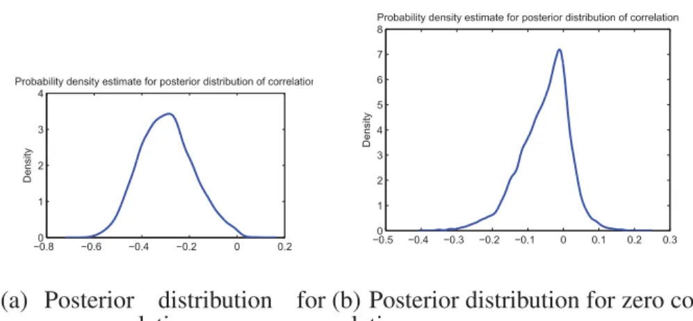
The Bayesian lasso model yields (adaptively) shrunk estimates of the precision matrix, whose entries are close to zero but not exactly zero i.e. the Laplace prior induces sparsity by shrinking the off-diagonal elementsCijclose to zero depending on the shrinkage parameter τij, but they will not be exactly zero. . To explore the zero entries in the precision matrix, we introduce a thresholding rule based on the variability of the estimates. We show this for the cork boring dataset example. The posterior kernel density estimates of the MCMC chains
for coefficients that were determined to be nonzero and determined to be exactly zero are as shown in Figures 1(a) and 1(b), respectively. To achieve sparsity, we compute the 95% bootstrap confidence interval for the mode ofCij from the MCMC samples of Cij. The mode for each data set of the bootstrap sample is computed by finding the kernel density for the sample and finding the mode of the estimated density. We use the method used in Botev et al. (2010) to automatically select the optimal bandwidth for density estimation. If zero is contained in the interval then the corresponding Cij is zero, and if zero is not
−0.80 −0.6 −0.4 −0.2 0 0.2 1 2 3 4 Density
Probability density estimate for posterior distribution of correlation
(a) Posterior distribution for nonzero correlation −0.50 −0.4 −0.3 −0.2 −0.1 0 0.1 0.2 0.3 1 2 3 4 5 6 7 8 Density
Probability density estimate for posterior distribution of correlation
(b) Posterior distribution for zero cor-relation
Fig. 1.: Shows the kernel density estimate of the empirical distributions of the MCMC samples of the correlations.
contained in the interval then the correspondingCij is the estimate of the mode. Generally the empirical distributions of the MCMC samples are unimodal, but in rare cases when they are multi-modal, the mode of the sample set is defined as the highest point in the empirical p.d.f. By using the method described above we get a graphical model that corresponds to
the model averaging of the best models, containing zero entries.
C. The Bayesian Lasso Selection Model for Sparse Graphical Models
In this section, we develop a selection model to identify the off-diagonal elements of the precision matrix that are exactly zero. We have a likelihood function for this model that is similar to the previous one as,
Y|G ∼ N(0,Ω−1, σ2In)
= (2πσ2)−np2 |Ω|n2exp{− 1
2σ2tr{ΩY Y
T}},
whereΩ=SCSis similarly structured as in the Bayesian lasso model, but the correlation matrixCis now modeled as
C =AR
whereis the Hadamard operator that does the element-wise multiplication.
1. Modelling the shrinkage matrixR
In order to achieve adaptive shrinkage of the partial correlations, we assign a Laplace prior to the off-diagonal elements ofR,Rij’s fori < j, where the Laplace prior is defined as
f(Rij|τij)∝ 1 2τij exp(−|Rij| τij ),
with each individual element having its own scale parameter, τij, that controls the level of sparsity. As discussed previously, Laplace priors have been widely used for shrinkage applications.
SinceRis a correlation matrix with elements that lie between [-1, 1], we incorporate this fact as an additional constraint on the overall convolution matrix,C ∈Cp, whereCp is the space of all correlation matrices of dimensionp. Hence the prior forRij can be written
as,
Rij|A∼Laplace(0, τij)I(C ∈Cp),
where the indicator function ensures that the correlation matrix is positive definite. The full specification of the constraints on theRij’s to ensure the positive definiteness are discussed in Appendix A.
In this setting, the shrinkage parameter τij controls the degree of sparsity, i.e., de-termines how much the ijth element of R will be shrunk towards zero. We assign an exchangeable inverse gamma prior as
τij ∼IG(e, f), i < j,
where(e, f) are the shape and scale parameters, respectively. Note that if we set τij = τ ∀i, j along with A = 1n (i.e., a matrix of all 1’s), this gives rise to the special case of the Bayesian version of the graphical lasso of Friedman et al. (2008) and Yuan and Lin (2007), where the single penalty parameter (τ) controls the sparsity of the graph and is estimated via cross-validation or by using a criterion similar to the Bayesian information criterion (BIC). By allowing the penalty parameter to vary locally for each node, we allow for additional flexibility, which has been shown to result in better properties than those of the lasso prior and which also satisfies the oracle property (consistent model selection), as shown by Griffin and Brown (2007) in the variable selection context. This fact is also illustrated in our data analysis and simulations studies.
2. Modelling the selection matrixA
Since A is the selection matrix that performs the variable selection on the elements of the correlation matrix R, it thus consists of only binary variables with the off-diagonal elements being either zeros or ones. The most general prior is an exchangeable Bernoulli
prior on the off-diagonal elements ofA, given as
Aij|qij ∼Bernoulli(qij), i < j,
whereqij is the probability that theijthelement will be selected as 1; and qij is assigned a beta prior as
qij ∼Beta(a, b), i < j.
In this construction the hyperparametersqij control the probability that the ijth ele-ment will be selected as a non-zero eleele-ment. To evaluate a highly sparse model the hyper-parameters should be specified such that the beta distribution is skewed towards zero, and for a dense model the hyper-parameters should be specified such that the beta distribution is skewed towards one. Furthermore, prior beliefs about the existence of edges can be in-corporated at this stage of the hierarchy by giving greater weights to important edges while down-weighting redundant edges.
In conclusion, the joint specification ofAandRabove gives us the graphical lasso selectionthat performs simultaneous shrinkage and selection. To complete the hierarchical specification of the graphical lasso selection, we use an inverse gamma prior on the inverse of the partial standard deviationsSi:
The complete hierarchical model can be succinctly summarized as Y|Ω, σ2 ∼ N(0,Ω−1, σ2In) Ω = S(AR)S Aij|qij ∼ Bernoulli(qij), i < j R|A ∼ i<j Laplace(0, τij)I(C ∈Cp) τij ∼ IG(e, f), i < j qij ∼ Beta(a, b), i < j Si ∼ IG(g, h) σ2 ∼ IG(k, l),
wherei= 1, . . . , p,j = 1, . . . , pandis the Hadamard product.
3. Conditional distributions and the posterior sampling for the selection model We again use MCMC methods for posterior inference as the joint posterior is not of ex-plicit form. All the full conditional distributions of the parameters are not in closed form, so we employ the MH algorithm to draw those parameters. For simplicity, let θij = {R−ij,A−ij, qij,Y} whereR−ij andA−ij contain all other off-diagonal elements of R andA, respectively, except theijthone.
Joint sampling of[Aij, Rij]:
First, we consider the complete conditional distribution ofRij as
[Rij|Aij, θij]∝ |Ω|n/2exp{− 1 2σ2tr{ΩY Y T} − 1 τij| Rij|}I(C ∈Cp)
We use this conditional distribution to drawRij. We use the discrete bootstrap method to drawRij similarly to drawingCij in the Bayesian lasso model. To sampleAij, we need to
evaluate its complete conditional distribution [Aij|Rij, θij]∝ |Ω|n/2exp{− 1 2σ2tr{ΩY Y T}}qAij ij (1−q 1−Aij ij )I(C ∈Cp) and use it to draw the binary variableAij.
An alternative way to sampleAij is to marginalizeRij from the joint distribution of Aij andRij and use the marginal distribution for sampling Aij. As the marginalization is not explicitly available, we use a Riemann approximation of this integral. We takeM grid points within the interval [uij, vij], which is the range of valuesRij can take, and use the approximation P(Aij = 0|θij)∝(1−qij) M k=1 |Ω(Rij(k),Aij=0)| n 2exp{−1 2σ2tr{Ω(Rij(k),Aij=0)Y Y T}} P(Aij = 1|θij)∝qij M k=1 |Ω(Rij(k),Aij=1)| n 2exp{−1 2σ2tr{Ω(Rij(k),Aij=1)Y Y T}}
Consequently, we drawAijas a discrete binary variable using these probabilities as weights.
Samplingτij, qij:
The full joint conditional distribution forτij andqij is
τij, qij|Aij, Rij, θij ∝K(τij, qij) 1 τij exp(−|AijRij| τij )×τij−g−1exp(− h τij ) ×qijAij(1−qij)(1−Aij)I(C ∈Cp),
whereKis the normalizing constant constrained by the truncation and positive definiteness constraint on C(= A R). First, based on R−ij we can identify the largest possible interval ofRij, sayuij andvij (Barnard et al. (2000)), which will keepCpositive-definite.
Then, we evaluateK(τij, qij): K−1(τij, qij) = Aij={0,1} qijAij(1−qij)(1−Aij) 1 −1 1 2τij exp{−|AijRij| τij }I[uij,vij](AijRij)dRij = (1−qij) 2 (vij −uij) τij I[uij,vij](0)IAij(0) + qij 2 CLap(uij, vij)I[uij,vij](Rij)IAij(1)
whereCLap(uij, vij) = [sgn(vij){1−exp{−| vij|
τij }} −sgn(uij){1−exp{
−|uij|
τij }}]andsgn
is the sign function
sgn(x) = ⎧ ⎪ ⎪ ⎪ ⎪ ⎪ ⎪ ⎨ ⎪ ⎪ ⎪ ⎪ ⎪ ⎪ ⎩ −1 ifx <0, 0 ifx= 0, 1 ifx >0.
Now we can drawτij andqij from their conditional distributions :
τij|qij, Aij, Rij,Y ∝K(τij, qij) 1 τij exp(−|AijRij| τij )×τij−g−1exp(− h τij ) qij|τij, Aij, Rij,Y ∝K(τij, qij)q aij ij (1−qij)(1−aij)qijα−1(1−qij)(β−1).
Both of these conditionals do not have an explicit form, so we need to use the Metropolis Hastings algorithm to drawτij andqij from their conditionals.
Samplingσ2:
The full conditional distribution of σ2 is in a closed form so we directly draw from the inverse gamma distribution as
k∗ =k+np/2, l∗ =l+ 1
2tr(ΩY YT)
SamplingSiThe full conditional distribution ofSi is Si|S−i,Y, σ2 ∝ |S(AR)S|n/2exp{− 1 2σ2tr{S(AR)SY Y T}}S−g−1 i exp( −h Si ) ∝Sinexp{− 1 2σ2tr{S(AR)SY Y T}} Si−g−1exp(−h Si ).
We use the Metropolis Hastings algorithm to sampleSi from this distribution.
4. Model selection using marginal probabilities
In this subsection, we propose a metric using marginal probabilities to compare different graphs visited by the MCMC chains. The marginal posterior probability of a given graphi-cal (G) structure can be expressed as,
p(G|Y)∝
p(Y|θ, G)p(θ|G)p(G)dθ, (1.1) whereY denotes the data andG encodes the variables that define the graphical structure andθrepresents all the other parameters in the model. In standard graphical modelsp(θ|G) is usually assigned a conjugate prior such as hyper Inverse-Wishart (Jones et al. (2004); Carvalho et al. (2007)) and hence the integral in (1.1) can be obtained explicitly. Although, making computations tractable, the conjugate priors restricts the search to to small classes of graphical models like decomposable graphical models (Giudici and Green (1999); Scott and Carvalho (2008)). In our framework, we explore a larger class of graphical models in addition to inducing sparsity which comes with an added computational complexity – the marginal density (1.1) is not available in explicit form.
However, one method to approximate the marginal posterior probability using our MCMC samples is as below.
1. We rank the top graphs based on some model selection criteria. For our examples we choose Bayes Information Criteria(BIC) which penalizes the complex models in
favor of balanced models and is defined as,
−2 logp(Y|G) +const≈ −2L(Y,θˆ) +mMlog(n)≡BIC
where p(Y|G) is the (integrated) likelihood of the data for the graph G, L(Y,θˆ) is the maximized mixture log likelihood for the model, and mG is the number of independent parameters to be estimated in the model. The number of parameters to be estimated in the model is considered as the number of nonzero edges and all the other parameters in the model.
2. Select topK (say 200) graphs in accordance with the BIC values.
3. Re-run the MCMC (for M iterations) to get sufficient samples to approximate the marginal probabilities using the Harmonic mean estimate (Newton and Raftery (1994); Gelfand and Dey (1994)).
4. Use the Harmonic mean estimateP(G|Y)≈(M−1iM=1p(Y|θi)−1)−1and normal-ize it to calculate the posterior probabilities of the models.
The resulting marginal posterior probabilities now come with appropriate uncertainty bounds and can be used for inference.
This approach has a major drawback which is the volatility of the harmonica mean estimators. This has been criticized widely in literature and we chose to use an alternative method to approximate posterior probabilities based on the frequency of appearance of models in the MCMC. We obtain the Monte-Carlo estimates of these posterior probabilities by counting the proportion of MCMC samples to have the specific graphical structure. Hence, ifI(A=A∗)denote the indicator function for the graphical modelA=A∗ , then
the ergodic average or the Monte Carlo frequency estimator of this modelA∗is given by π(A∗|Y) = 1 K K b=1 I(Ab =A∗),
whereAbis graphical model visited on thebthMCMC draw andK is the total number of draws from the Markov chain.
D. A Naive Bayesian Model
We also develop a naive Bayesian model expressingCas
C =ARˆ,
whereis the Hadamard operator that does element wise multiplication. HereRˆis a plug-in estimate of the correlation matrix obtaplug-ined from factorizplug-ing the estimate of the precision matrixΩˆ = ˆSRˆSˆwhereRˆ is a correlation matrix andSˆis a diagonal matrix. The relation ofRˆ to partial correlation is described in Subsection C. For a relatively large sample size, the inverse of the sample correlation matrix is an obvious choice for this estimate.Ais the shrinkage matrix such that the elements ofA will shrink the elements inRˆ. In this way some of the elements ofRˆ will be shrunk towards0. This approach is similar in spirit to the nonnegative garrote estimator proposed by Breiman (1995) and Yuan and Lin (2007).
We assign a Laplace prior on the off-diagonal elements ofA
Aij ∼Laplace(0, τ), i < j.
E. Simulations
In this subection we compare different methods to assess the performance of the Bayesian lasso models. We simulate five types of concentration matrices, in order of increasing structural complexity:
1. Identity matrix
2. Banded diagonal matrix.
3. Block diagonal matrix 4. Sparse unstructured matrix.
5. Dense unstructured matrix.
An identity matrix is a simple matrix with ones in its diagonal and zeros in its off diagonal. Banded diagonal matrix is a tridiagonal matrix with ones in its diagonal and all the elements in the diagonals adjacent to the main diagonal set to 0.5. Before explaining simulations of more complex matrix structures, we describe the process used for generating a random positive definite correlation matrix. A random lower triangular matrix L was generated with ones in its diagonal and normal random numbers in its lower triangle. ThenLLT gave us a positive definite matrix. The matrix was then factored asQΩQ, whereQis a diagonal matrix andΩis a correlation matrix with ones in its diagonal which is the desired positive definite correlation matrix. A block diagonal matrix was generated as follows. Two positive definite matrix correlation matrices of sizesp−kandkwere generated, where k is a random number between1andp, and were concatenated in the diagonals to create a matrix of size p×pas shown in Figure 2(c). the sparse unstructured matrix was simulated as follows: Let
Σ = B+δIp where each off-diagonal entry inB is generated independently and equals a random number between [−1,−.5] and [.5,1] with probability π or 0 with probability
2 4 6 8 10 1 2 3 4 5 6 7 8 9 10
(a) Identity Matrix
2 4 6 8 10 1 2 3 4 5 6 7 8 9 10
(b) Banded Diagonal Ma-trix 2 4 6 8 10 1 2 3 4 5 6 7 8 9 10
(c) Block Diagonal Ma-trix 2 4 6 8 10 1 2 3 4 5 6 7 8 9 10 (d) Sparse Matrix 2 4 6 8 10 1 2 3 4 5 6 7 8 9 10 −1 −0.8 −0.6 −0.4 −0.2 0 0.2 0.4 0.6 0.8 1
(e) Dense Matrix
Fig. 2.: This figure shows the simulated matrices for different types of structures for pre-cision matrix. The colorbar is same for all the matrices. White indicates a zero in the precision matrix whereas colored cells indicate non-zero elements.
1−π, all diagonal entries of Bare zero and δis chosen such that the resulting matrix is positive definite. In the end we do the factorization of ΣasQΩQ, whereQis a diagonal matrix andΩis a correlation matrix with ones in its diagonal, which is the desired sparse positive definite correlation matrix. We can vary the sparsity of the matrices generated by changing the value ofπ. We choseπ = 0.1for the sparse unstructured matrix. The dense unstructured matrix is the full matrix that is a random positive definite correlation matrix of sizepgenerates using the method described above. The simulated matrices for sizep= 10
are shown in Figure 2. In Figure 2 the white blocks in the off diagonal are the zeros in the matrices, the colors correspond to the magnitude of nonzero off-diagonal elements in the matrices as represented by the colorbar at the end of the figure.
We compare our methods with the “glasso” approach of Friedman et al. (2008) and the method (“MB”) proposed by Meinshausen and B´uhlmann (2006) as both these methods use the L1- regularization and are closest to our approach using Laplace priors. We try to assess the performance of these methods in terms of the Kullback-Leibler loss (KL), the number of false positives (FP; incorrectly identified edges) and the number of false negatives (FN; incorrectly missed edges). Both the methods were implemented using the glasso package in R. We implemented them using Matlab-R link to call the the functions in Matlab.
It should be noted that both these methods are frequentist methods and they give a point estimate for the precision matrix, whereas the Bayesian methods can also provide the uncertainty estimates for the covariance matrix, so we are comparing the performance regarding the final estimate of the precision matrix. For the Bayesian lasso model and the Bayesian lasso selection model we use the estimate of the precision matrix as the matrix that has the highest joint log posterior of all of the unique models visited in the MCMC simulation. The joint log posterior is computed at every iteration of the MCMC simulation, and the sample with the highest joint log posterior is the most likely map estimate, which can be compared with the estimates of the above two frequentist methods.
The Kullback -Leibler Loss is defined asΔKL( ˆΩ,Ω) =trace(ΩΩˆ−1)−log|ΩΩˆ−1|− p, whose ideal value should be zero whenΩˆ =Ω. Figures 3, 4 and 5 show the means and standard errors for the KL, FP and FN for sample sizen={25}and number of covariates p={5,10,15,25}averaged over 10 data sets.
The “glasso” method and the “MB” method were performed usingρ = 0.1which is the tuning parameter for the lasso penalty in both the methods because this setting gave good results for all the scenarios. As shown in Figure 3, the proposed Bayesian methods
perform better than the other methods in some of the cases while in others all the methods are competitive with each other. The Bayesian Lasso model does better than the Bayesian lasso selection model in simpler correlation structures as the Bayesian lasso is a shrinkage model from which the zeros were selected post-MCMC. As it is a continuous model it has a better probability to get to good estimate of the precision matrix in simpler models such as the identity matrix structures, where as the Bayesian lasso selection model is more of a model searching method which searches over all the models of the precision matrix to find which are the probable models. The Bayesian lasso has a higher probability of getting stuck in a local mode than the Bayesian lasso selection model. As the Bayesian lasso selection model makes discrete jumps in the model space, it is more likely to explore the whole space.
We can see that all the methods perform more or less the same in Identity and Dense Matrix structures. In sparse unstructured matrices and banded diagonal matrices the Bayesian models outperform the “glasso” and “MB” methods. This is because of the adaptive regu-larization on the partial correlations in Bayesian models. If “glasso” and “MB” did adaptive regularization the methods would have been competitive with each other in these scenarios.
To compute the false positive and false negative rate for the Bayesian lasso model we need to use the bootstrap confidence intervals to find the zeros in the model. This is not necessary for the Bayesian lasso selection model as the zeros are directly incorporated in the model. We also computed the false negative and false positive rates for the methods and compared them in Figures 5 and 4 respectively. This is mostly dependent on the parameter for tuning the sparsity. If you want more sparser models you are more likely to get false negatives and less likely to get false positives. All the methods have similar false negative rates except for dense and block diagonal matrices. Both these scenarios are dense matrices so there are a lot of elements in the matrix which have small partial correlations but not exactly zero, so all the models are likely to make them zero as they are small enough. So there is a higher chance of getting a false negative in these scenarios than others. For the scenario of Identity matrices there is no chance of getting a false negative as all elements are zeros.
The false positive rates tell us how likely you are to make an error by changing an element which was actually zero to a nonzero one. We can see that the Bayesian models have smaller false positive rates compare to the “glasso” and “MB” methods.
0 5 10 15 20 25 30 −1 0 1 2 3 4 5 No of covariates p Kullback − Leibler Loss
Comparison between methods for Identity Matrices Bayesian Lasso
Bayesian Lasso Selection glasso
MB
(a) Identity Matrix
0 5 10 15 20 25 30 0 5 10 15 20 25 30 35 40 No of covariates p Kullback − Leibler Loss
Comparison between methods for Banded Tridiagonal Matrices Bayesian Lasso
Bayesian Lasso Selection glasso
MB
(b) Banded Diagonal Matrix
0 5 10 15 20 25 30 0 2 4 6 8 10 12 14 16 18 20 No of covariates p Kullback − Leibler Loss
Comparison between methods for Block Diagonal Matrices Bayesian Lasso
Bayesian Lasso Selection glasso
MB
(c) Block Diagonal Matrix
0 5 10 15 20 25 30 0 5 10 15 20 25 No of covariates p Kullback − Leibler Loss
Comparison between methods for Sparse Unstructured Matrices Bayesian Lasso
Bayesian Lasso Selection glasso MB (d) Sparse Matrix 0 5 10 15 20 25 30 0 2 4 6 8 10 12 14 16 18 20 No of covariates p Kullback − Leibler Loss
Comparison between methods for Dense Unstructured Matrices Bayesian Lasso
Bayesian Lasso Selection glasso
MB
(e) Dense Matrix
Fig. 3.: This figure shows the comparison between 4 methods “glasso” -Friedman et al. (2008), “MB”- Meinshausen and B´uhlmann (2006), “Bayesian lasso” model and “Bayesian lasso selection” model in terms of Kullback-Leibler loss (K-L) for the simulated simulated matrices for different types of structures for precision matrix forp= 25. Lower is better.
0 5 10 15 20 25 30 −0.1 0 0.1 0.2 0.3 0.4 0.5 0.6 0.7 0.8 No of covariates p
False Positive Rate
Comparison between methods for Identity Matrices Bayesian Lasso Bayesian Lasso Selection glasso
MB
(a) Identity Matrix
0 5 10 15 20 25 30 −0.05 0 0.05 0.1 0.15 0.2 0.25 0.3 0.35 0.4 0.45 No of covariates p
False Positive Rate
Comparison between methods for Banded Diagonal Matrices Bayesian Lasso Bayesian Lasso Selection glasso
MB
(b) Banded Diagonal Matrix
0 5 10 15 20 25 30 −0.1 0 0.1 0.2 0.3 0.4 0.5 0.6 No of covariates p
False Positive Rate
Comparison between methods for Block Diagonal Matrices Bayesian Lasso Bayesian Lasso Selection glasso
MB
(c) Block Diagonal Matrix
0 5 10 15 20 25 30 −0.1 0 0.1 0.2 0.3 0.4 0.5 0.6 No of covariates p
False Positive Rate
Comparison between methods for Sparse Unstructured Matrices Bayesian Lasso Bayesian Lasso Selection glasso MB (d) Sparse Matrix 0 5 10 15 20 25 30 −0.05 0 0.05 0.1 0.15 0.2 No of covariates p
False Positive Rate
Comparison between methods for Dense Unstructured Matrices Bayesian Lasso
Bayesian Lasso Selection glasso
MB
(e) Dense Matrix
Fig. 4.: This figure shows the comparison between 4 methods “glasso” -Friedman et al. (2008), “MB”- Meinshausen and B´uhlmann (2006), “Bayesian lasso” model and “Bayesian lasso selection” model in terms of false positive rates for the simulated simulated matrices for different types of structures for precision matrix forp= 25. Lower is better.
0 5 10 15 20 25 30 −1 −0.8 −0.6 −0.4 −0.2 0 0.2 0.4 0.6 0.8 1 No of covariates p
False Negative Rate
Comparison between methods for Identity Matrices Bayesian Lasso
Bayesian Lasso Selection glasso
MB
(a) Identity Matrix
0 5 10 15 20 25 30 −0.04 −0.02 0 0.02 0.04 0.06 0.08 0.1 No of covariates p
False Negative Rate
Comparison between methods for Banded Diagonal Matrices Bayesian Lasso
Bayesian Lasso Selection glasso
MB
(b) Banded Diagonal Matrix
0 5 10 15 20 25 30 0 0.02 0.04 0.06 0.08 0.1 0.12 0.14 0.16 0.18 No of covariates p
False Negative Rate
Comparison between methods for Block Diagonal Matrices Bayesian Lasso
Bayesian Lasso Selection glasso
MB
(c) Block Diagonal Matrix
0 5 10 15 20 25 30 −0.04 −0.02 0 0.02 0.04 0.06 0.08 0.1 0.12 0.14 0.16 No of covariates p
False Negative Rate
Comparison between methods for Sparse Unstructured Matrices Bayesian Lasso
Bayesian Lasso Selection glasso MB (d) Sparse Matrix 0 5 10 15 20 25 30 0 0.1 0.2 0.3 0.4 0.5 0.6 0.7 0.8 0.9 No of covariates p
False Negative Rate
Comparison between methods for Dense Unstructured Matrices Bayesian Lasso
Bayesian Lasso Selection glasso
MB
(e) Dense Matrix
Fig. 5.: This figure shows the comparison between 4 methods “glasso” -Friedman et al. (2008), “MB”- Meinshausen and B´uhlmann (2006), “Bayesian lasso” model and “Bayesian lasso selection” model in terms of false negative rates for the simulated simulated matrices for different types of structures for precision matrix forp= 25. Lower is better.
F. Model Comparison with Benchmark Data
We chose to compare our methods with three existing methods that were earlier used in different papers. The Lasso and non negative type garrotte estimator are used in Yuan and Lin (2007) and Mixed Interaction Modeling (MIM) is one of the leading softwares for graphical modeling. For determining the best models for Bayesian lasso model we use the model obtained with the bootstrap confidence intervals. For the Bayesian lasso selection model we compute the joint log posterior for all of the unique models visited in the MCMC simulation and we select the model with the highest joint log posterior as the best model.
Lasso Model: The Lasso model is a penalized-likelihood method that does model selection and parameter estimation simultaneously in the Gaussian concentration graph model and uses anL−1penalty on the off-diagonal elements of the concentration matrix that encourages encourages sparsity and simultaneously shrinks the estimates.
Non-Negative Garrote Model: This model is similar to the Lasso model but the fact that we have a relatively reliable estimate of the concentration matrix changes the penalty function by incorporating the estimate into it (Yuan and Lin (2007)). This approach is similar to the non-negative garrote estimator proposed by Breiman (1995) for linear regression.
MIM: MIM is the only available software supporting graphical modeling with both discrete and continuous variables. MIM is designed for graphical modeling using undi-rected graphs, diundi-rected acyclic graphs and chain graphs. It is based on a comprehensive class of statistical models for discrete and continuous data. The dependence properties of the models can be displayed in the form of a graph. The backward stepwise selection method in Edward‘s MIM package with the option of unrestricted selection, wherein both decomposable and non-decomposable models are considered, is used. Implementation of the stepwise model selection procedure in MIM is based on removing only one edge, the
least significant one, at a time.
1. Examples
We consider two benchmark real datasets and a stock market dataset to compare our meth-ods
a. Example 1: Cork borings data set
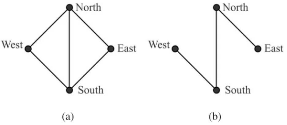
Cork borings data are presented in Whittaker (1990)(Exercise 8.6.5) and were originally used by Rao (1948). Thep = 4measurements are the weights of cork borings onn = 28 trees in four directions: north, east, south and west.
(a) (b)
Fig. 6.: (A) was selected by Lasso, Garrote and Naive Bayes Models and (B) was selected by Bayesian lasso, Bayesian lasso selection and MIM Models.
Figure 6 depicts the best graphs for the cork borings data set. We can see that the Bayesian lasso, Bayesian lasso selection and MIM models select the same graph, Figure 6(b) as the best graph. This graph had the highest joint posterior value for both the Bayesian lasso and Bayesian lasso selection models. Whereas the graph in Figure 6(a) is selected as the best graph by Lasso, Garrote and Naive Bayes models. As these are benchmark datasets