This is a repository copy of Bayesian inference of multivariate rotated GARCH models with skew returns.
White Rose Research Online URL for this paper: http://eprints.whiterose.ac.uk/146215/
Version: Accepted Version Article:
Iqbal, F. and Triantafyllopoulos, K. orcid.org/0000-0002-4144-4092 (2019) Bayesian inference of multivariate rotated GARCH models with skew returns. Communications in Statistics - Simulation and Computation. ISSN 0361-0918
https://doi.org/10.1080/03610918.2019.1620272
This is an Accepted Manuscript of an article published by Taylor & Francis in
Communications in Statistics - Simulation and Computation on 29/05/2019, available online: http://www.tandfonline.com/10.1080/03610918.2019.1620272
Reuse
Items deposited in White Rose Research Online are protected by copyright, with all rights reserved unless indicated otherwise. They may be downloaded and/or printed for private study, or other acts as permitted by national copyright laws. The publisher or other rights holders may allow further reproduction and re-use of the full text version. This is indicated by the licence information on the White Rose Research Online record for the item.
Takedown
If you consider content in White Rose Research Online to be in breach of UK law, please notify us by
Bayesian inference of multivariate rotated
GARCH models with skew returns
Farhat Iqbal and Kostas Triantafyllopoulos
Department of Statistics, University of Balochistan, Quetta, Pakistan
and School of Mathematics and Statistics,
Hicks Building, University of Sheffield, S3 7RH, Sheffield, UK
email:
[email protected]
, Tel: +44 114 222 3741
May 10, 2019
Abstract
Bayesian inference is proposed for volatility models, targeting fi-nancial returns, which exhibit high kurtosis and slight skewness. Ro-tated GARCH models are considered which can accommodate the multivariate standard normal, Student t, generalised error distribu-tions and their skewed versions. Inference on the model parame-ters and prediction of future volatilities and cross-correlations are ad-dressed by Markov chain Monte Carlo inference. Bivariate simulated data is used to assess the performance of the method, while two sets of real data are used for illustration: the first is a trivariate data set of financial stock indices and the second is a higher dimensional data set for which a portfolio allocation is performed.
Keywords: Volatility, skew returns, GARCH, BEKK, rotated BEKK, multivariate time series, portfolio allocation.
1
Introduction
The time-varying dynamics of conditional covariances of asset returns play a crucial role for asset pricing, portfolio allocation and risk management and hence their modelling and forecasting has gained considerable attention for the past three decades. Multivariate generalised autoregressive conditional heteroscedastic (MGARCH) models have been routinely used to study and examine the relationship between the volatilities and co-volatilities of multi-variate financial time series.
A wide range of MGARCH models have been proposed in the literature to accommodate time-varying multivariate volatility but the number of parame-ters increases rapidly as the the dimension of the returns grows; this is widely known as thecurse of dimensionality, see e.g. Bauwens et al. (2006) and Sil-vennoinen and Ter¨asvirta (2009), among others. Bollerslev et al. (1988) first introduced the half-vec (vech) form for the conditional covariance matrices and its special case is the popular Baba-Engle-Kraft-Kroner (BEKK) model of Engle and Kroner (1995). Though the BEKK model provides rich dynam-ics of conditional covariances, the estimation of this model demands heavy computations. The diagonal BEKK model, where parameter-matrices are assumed diagonal, provides some simplification over the full BEKK model. Several models have been proposed in the literature based on transforma-tions of the returns (van der Weide, 2002; Fan et al., 2008; Boswijk and van der Weide, 2011). Noureldin et al. (2014) proposed the rotated BEKK
(RBEKK) model that utilises the BEKK parametrisation using covariance targeting and aiming at higher dimensional data by exploiting returns rota-tion. With respect to estimation, maximum likelihood is usually adopted to carry out inference of multivariate GARCH-type models. On the other hand, the Bayesian paradigm is well suited for MGARCH models and provides cer-tain advantages in comparison to the llikelihood-based inference. Several papers have adopted Bayesian estimation, in particular Markov chain Monte Carlo (MCMC) inference, see e.g. Vrontos et al. (2003), Osiewalski and Pipien (2004) and the review of Virbickaite et al. (2015).
The main contribution of the article is to develop a Bayesian approach for the estimation of the parameters of the RBEKK models allowing for heavy-tailedness and asymmetry in the distribution of the returns. Under a Bayesian framework, a block-sampling MCMC scheme is proposed for the es-timation of the rotated volatility covariance matrix. Results of Monte Carlo simulations show that the method accurately estimates the volatilities and correlations of multivariate returns. The model is first evaluated via a bi-variate simulated data set; for this data set the true simulated volatilities, correlations and model parameters are always within the in-sample credible intervals, which are remarkably narrow. Consequently, an empirical study is considered for a trivariate data set consisting of Frankfurt (Dax), Paris (Cac40) and Tokyo (Nikkei) stock indices. Finally, a higher dimensional data set is analysed consisting of eight shares from Dow Jones industrial average index, for which an asset allocation is performed and its evaluation is
con-ducted using cumulative portfolio returns. The assessment and performance of the model suggest very accurate in-sample and volatility forecasting pro-viding clearly improved performance in comparison to maximum likelihood estimation. The utility of this paper is to offer MCMC inference for the volatility of financial returns, which exhibit heavy tails and asymmetry; the covariance targeting approach allows the estimation of higher dimensional data sets.
The structure of the remainder of the article is as follows. In Section 2, we discuss the specification of the MGARCH model and the rotated BEKK models. Section 3 describes in detail the proposed Bayesian inference and forecasting for the RBEKK model. Results of simulation studies are pre-sented in Section 4 and application to the real data sets are discussed in Section 5. Finally, the paper concludes with closing comments.
2
Multivariate GARCH models
Consider a general multivariate GARCH model
rt=H1t/2εt, (1)
where rt = (r1t,· · · , rKt)′, t = 1,2, . . . , T, is a K-dimensional daily asset
returns, εt is a K-dimensional i.i.d process with mean zero and identity covariance matrix. This model assumes a zero-mean E[rt|Ωt−1] = 0 and
conditional covariance matrix E[rtr′t|Ωt−1] = Ht, with elements Hij,t, i =
j = 1, . . . , K, where Ωt−1 denotes the information set at time t− 1 and
E[·] denotes expectation. A parametrisation for the conditional covariance matrix Ht completes the multivariate GARCH model.
One of the most widely used models for the conditional covariances adopts the BEKK specification
Ht=CC ′ +Art−1r ′ t−1A ′ +BHt−1B ′ , (2)
where C,A and B are K ×K square matrices with C being a positive def-inite symmetric parameter matrix. The fully parameterised model includes 2.5K2+ 0.5K parameters and only feasible for small value of K.
Noureldin et al. (2014) propose a rotated version of the above model, the rotated BEKK (RBEKK) model that utilises the BEKK parametrisation using covariance targeting. More specifically, the model is fitted using the rotated returns ˜rt=H∗−1/2 rt=PΛ−1/2 P′ rt, (3) where H∗ =PΛP′
is the unconditional covariance of rt and the matrices of eigenvectors P and eigenvalue Λare obtained using spectral decomposition. Now, the unconditional covariance matrix of rotated returns ˜rt is Var[˜rt] =
covariance-targeting the conditional covariance matrix of ˜rt is defined as Gt = (IK−A˜A˜ ′ −B˜B˜′ ) + ˜A˜rt−1˜r ′ t−1A˜ ′ + ˜BGt−1B˜ ′ , (4)
with G0 = IK and assume (IK −A˜A˜′ − B˜B˜′) ≥ 0 on the sense of being
positive semidefinite. The RBEKK model is the restricted BEKK model with parameters A∗ =H∗1/2˜ AH∗−1/2 , B∗ =H∗1/2˜ BH∗−1/2 and C∗ =H∗1/2 (IK− ˜ AA˜′ −B˜B˜′ )H∗1/2
. A high-order lag structure or asymmetric term can also be introduced in (4).
Noureldin et al. (2014) study three different specifications of RBEKK models called scalar RBEKK (S-RBEKK), diagonal RBEKK (D-RBEKK) and common persistence RBEKK (CP-RBEKK). Here, we discuss the scalar and diagonal specifications. The scalar specification assumes ˜A = α1/2I
K
and ˜B =β1/2I
K. The (i, j)th element of Gt is given by
gij,t= (1−α−β)I(i=j)+αr˜i,t−1r˜j,t−1 +βgij,t−1, i, j = 1, . . . , K,
where I(·) is the indicator function. Note that in this specification, all the
elements ofGthave the same dynamic parameters. It is assumed thatα, β ≥
0 and α+β <1 is required for covariance stationarity. The total number of parameters is 2 in the scalar specification.
In the diagonal specification, ˜A and ˜B are diagonal with elements α1ii/2
specification implies gij,t =(1−α1ii/2α 1/2 jj −β 1/2 ii β 1/2 jj )I(i=j)+α1ii/2α 1/2 jj r˜i,t−1r˜j,t−1 +βii1/2βjj1/2gij,t−1, i, j = 1, . . . , K.
Assuming α1ii/2 > 0 and βii1/2 > 0 along with αii +βii < 1 ensure that
(IK −A˜A˜′ −B˜B˜′) is positive definite. The total number of parameters to
be estimated in the D-RBEKK model is 2K.
It is noted that the BEKK and REBEKK models have the same num-ber of parameters. The diagonal RBEKK model implies a full BEKK model for returns. Besides, fitting a diagonal RBEKK model implies rather rich dynamics for the unrotated returns (Noureldin et al. 2014, p. 18). The transformation of the raw returns enables the fitting of flexible multivariate models to the rotated returns using covariance targeting (Noureldin et al., 2014). Since the diagonal BEKK model implies a full BEKK model for unro-tated returns, fitting this model provides rich dynamics with smaller number of parameters. This may be attractive for modelling both the volatilities and correlations in large dimensions as only 2K dynamic parameters need to be estimated in the diagonal specification.
3
Bayesian inference for RBEKK Models
3.1
Preliminaries
Estimation of the RBEKK models involves a two-step estimation procedure. In the first step, a method of moment estimator is used to obtain an estimate of the rotated volatility matrix H∗
: b H∗ =T−1 T X t=1 rtr ′ t. By noting that H∗ = PΛP′
(see equation (3)), this estimator can be de-composed into Pb and Λb to obtain the rotated returns ˜rt =PbΛb−1/2Pb′
rt, t= 1,2, . . . , T.
In the second step, we adopt a Bayesian approach to estimate the pa-rameters of RBEKK models with skewed and heavy-tailed distributions for the errors by constructing MCMC algorithms. The conditional likelihood function for model (1) can be written as
L(θ;r) = T Y t=1 |Ht| −1/2 pε(H −1/2 t rt), (5) where r = (r′ 1, . . . ,r ′ T) ′
is the sample of returns and pε is the joint density
function for εt, and θ is the vector of unknown parameters in the model.
The likelihood function for (3) can be defined in a similar manner.
on the rotated conditional covariance matrix). This enables the study of un-certainty around the volatility of the rotated returns, but it does not provide uncertainty around the the matrix transformation in order to obtain the ro-tated returns. Joint Bayesian estimation of the conditional returns and the unconditional returns might be possible, but it is not explored in this paper any further. Markov chain Monte Carlo estimation of the unconditional re-turns in Step 1 would negate the advantage of the reduction of parameters in the model. One possibility to move forward this idea is to estimate the unconditional covariance volatility matrix in the first step by employing par-ticle filters (Creal, 2012) and then to adopt the proposed MCMC approach for the estimation of the conditional returns in the second step.
3.2
Asymmetric error distribution
The standardised multivariate normal or Student t distributions are often used for the error distribution; the latter being capable to describe heavy tailed returns, which are typically observed in finance. However, as it is common for financial returns to exhibit asymmetry a suitable asymmetric error distribution may be considered. Bauwens and Laurent (2005) describe a method of constructing a multivariate skew distribution from a symmetric one. They show that the multivariate skew densities can be written as
s(x|γ) = 2K K Y i=1 γi 1 +γ2 i ! f(x∗ ),
where f(·) is a symmetric multivariate density, x∗ = (x∗ 1, . . . , x ∗ K) ′ , γi > 0
is the shape parameter, x∗
i = xiγiIi, i = 1, . . . , K, with Ii = −1, if xi ≥ 0,
and 1 otherwise, being the indicator function. Note that γi = 1 yields the
symmetric distribution, γi >1(<1) indicates right (left) skewness and γi2 =
P r(xi ≥0)/P r(xi <0) (Fernandez and Steel, 1998). The first two moments
of x∗ i are given by mi =Mi,1 γi− 1 γi , (6) si = Mi,2−Mi,21 γi2+ 1 γ2 i + 2Mi,21−Mi,2, (7) with Mi,r = Z ∞ 0 2urfi(u)du.
The log-likelihood function for multivariate skew-normal distribution is
L(θ) =− 1 2 T X t=1 log|Ht|+ K X i=1 si K X j=1 pij,trj,t+mi 2 γ2Ii i +T XK i=1
(logγi+ logsi)−log(1 +γi2)
+T K
2 [log(2)−log(π)], (8)
wherepij,tcorresponds to thejthelement of theithrow of the inverse Cholesky
factor of the matrix Ht.
The multivariate generalised error distribution (GED) can also be used as an alternative heavy tailed distribution. For the GED, the tail parame-ter δ needs to be estimated along with other parameters. The multivariate
standard normal is obtained for δ = 2 and the value δ < 2(> 2) leads to thicker (thinner) tails than the standard normal (see Fioruci et al., 2014 for further discussion on univariate and multivariate skew distributions). For expressions of the likelihood function of models with skew tand GED return distributions the reader is referred to Braione and Scholtes (2016) and to references therein.
3.3
Markov chain Monte Carlo estimation
Let θ denote the set of all unknown parameters which includes the param-eters of RBEKK models, (α1/2, β1/2) in case of the scalar specification and
(α111/2, . . . , α1KK/2, β111/2, . . . , βKK1/2) in case of the diagonal, the shape parameters for each returns (γ1, . . . , γK) and the tail parameter ν or δ when using the
multivariate Student t or GED, respectively.
In a Bayesian framework (Chib and Greenberg, 1995) prior distributions for all parameters of interest need to be specified. These are assumed to
be a priori independent and normally distributed truncated to the intervals
they are defined. We focus our attention on the diagonal specification as this provides rich dynamics compared to the scalar specification. For α1ii/2 and
βii1/2, i = 1, . . . , K, we assume αii1/2 ∼ N(µα1/2 ii , σ 2 α1ii/2)I(0<α1ii/2<1) and β 1/2 ii ∼ N(µβ1/2 ii , σ 2
β1ii/2)I(0<βii1/2<1). A prior distribution for the tail parameter (the
degrees of freedom) is ν ∼N(µν, σν2)I(ν>2), for the multivariate Studentt or
δ ∼ N(µδ, σ2δ)I(δ>0), for multivariate GED. The choice of prior distribution
N(0,0.64−1
)I(γi>0). The values for hyper parameters are specified asµαii =
µβii = µν = µδ = 0 and σ 2 αii = σ 2 βii = σ 2
ν = σδ2 = 100. The relatively large
variances reflect on a weakly informative prior specification; it is possible to set up a hierarchical prior structure by specifying an inverse prior distribution for each variance, but there was little benefit in the estimation and this approach was not adopted to avoid extra computation cost.
A block Metropolis-Hastings algorithm is constructed to sample from the posterior distributionp(θ|rt) where all the parameters are updated as a block.
More specifically, a random walk Metropolis algorithm is used where at each iteration a new vector from a multivariate normal distribution centred around the current vector with a variance-covariance proposal matrix is generated. The proposal matrix is calculated from a pilot tuning that is carried out by running one-dimensional random walk Metropolis updates with univariate normal candidate distributions whose variances are calibrated to obtain good acceptance rates. The main steps of the algorithm are:
1. Initialize the parameter vector θ0 and set n= 0.
2. Draw a sample θ(n+1) from the distribution ofθ|rt.
3. Setn =n+ 1 and go to step 2, untiln =N, for a large N.
In step 2 we sample from the conditional posterior distribution of θ whose kernel is given by
where p(θ) is the prior probability of θ. The random walk Metropolis-Hastings method is used for this purpose as described in the following two steps:
First, we generate a candidate vector ˜θ from the multivariate normal distribution N(θ(n), cΣbθ), where c is a constant and Σbθ is the covariance matrix calculated from a pilot tuning. Let
τθ(n)= min{1,(κ(˜θ|rt))/(κ(θ(n)|rt))},
where κ(˜θ|rt) is given in eq. (9). Then, define θ(n+1) = ˜ θ, with probability τθ(n) θ(n) with probability 1−τθ(n)
The constantcis used to tune the acceptance rate (usually lying between 0.2 and 0.5) to achieve fast convergence. This builds an irreducible and aperiodic Markov chain in the parameter space θ(0),θ(1), . . . ,θ(N). For large N, θ(n)
tends in distribution to a random variable with density p(θ|rt).
4
Simulation studies
In this section, we study the performance of the proposed MCMC sampler for the RBEKK model through Monte Carlo simulations. We performed
two simulation studies on the bivariate diagonal RBEKK model. Samples of sizes T = 2000 and T = 5000 were simulated from this model. The true parameter vector for the bivariate RBEKK model (equations (3) and (4)) with diagonal specification is set to θ = (α111/2 =√0.05, α221/2 =√0.10, β111/2 =
√
0.90, β221/2 = √0.80). Note that the diagonal specification assumes that ˜
A = diag{α1ii/2} and ˜B = diag{βii1/2}, for i = 1,2. For the sake of brevity, results for errors from the multivariate skew t distribution, ST(ν,γ), with
ν = 8 are only reported. For the shape parameter, we selected negatively skewed errors with γ = (0.8,0.8)′
. Such a setting generates heavy tailed and skewed returns that are commonly observed in financial time series.
The proposed MCMC algorithm is then used to estimate the parame-ters of the diagonal RBEKK model for each simulated series. The MCMC algorithm is run using N = 20000 iterations discarding the initial 10000 it-erations as burn-in samples. Geweke convergence diagnostic (Geweke, 1992) were used to check the convergence of the Markov chains. The MCMC chains provide good mixing performance and fast convergence.
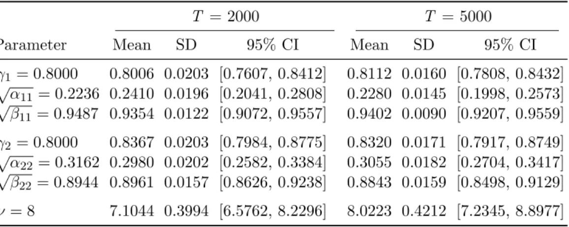
Table 1 shows posterior means, standard deviations and 95% credible intervals of the model parameters for the two simulated series. Observe the accuracy of the estimation and note that the 95% credible intervals al-ways include the true parameters. The posterior standard deviations become smaller as the sample size increases and the length of the credible intervals decrease reflecting upon precision. Besides the availability of point estimates, Bayesian estimation routinely provides parameter uncertainty, e.g. via the
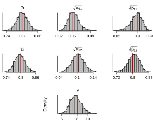
γ1 Density 0.74 0.8 0.86 α11 0.02 0.05 0.09 β11 0.82 0.9 0.94 γ2 Density 0.74 0.8 0.86 α22 0.04 0.1 0.14 β22 0.72 0.8 0.88 ν Density 5 8 10
Figure 1: Histograms and density of the posterior MCMC samples of model pa-rameters of the first simulated series with T = 2000. Vertical line represents the true value of the parameter.
empirical posterior densities. This parameter uncertainty may be introduced in the estimation of volatilities, correlations, value-at-risk (VaR), portfolio selection, and so on. The histograms and densities of the posterior samples of each parameter for the first simulated series with sample size T = 2000 is shown in Figure 1. The histograms for large sample size T = 5000 (not re-ported) exhibit higher degree of symmetry and smaller variance as compared to those of size T = 2000.
pre-Table 1: Estimates of the model parameters with multivariate skewterrors.
T = 2000 T = 5000
Parameter Mean SD 95% CI Mean SD 95% CI
γ1 = 0.8000 0.8006 0.0203 [0.7607, 0.8412] 0.8112 0.0160 [0.7808, 0.8432] √α 11= 0.2236 0.2410 0.0196 [0.2041, 0.2808] 0.2280 0.0145 [0.1998, 0.2573] √ β11= 0.9487 0.9354 0.0122 [0.9072, 0.9557] 0.9402 0.0090 [0.9207, 0.9559] γ2 = 0.8000 0.8367 0.0203 [0.7984, 0.8775] 0.8320 0.0171 [0.7917, 0.8749] √α 22= 0.3162 0.2980 0.0202 [0.2582, 0.3384] 0.3055 0.0182 [0.2704, 0.3417] √ β22= 0.8944 0.8961 0.0157 [0.8626, 0.9238] 0.8843 0.0159 [0.8498, 0.9129] ν = 8 7.1044 0.3994 [6.5762, 8.2296] 8.0223 0.4212 [7.2345, 8.8977]
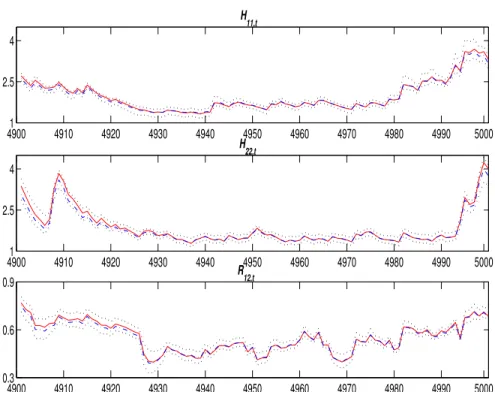
sented in Figure 2. The estimated in-sample volatilities, Hbii,t, for i = 1,2,
and the in-sample correlations,Rb12,t,for last 1000 observations,t= 4901, . . . ,
5000 for the simulated series with T = 5000 are presented. True values for volatilities and correlations along with 95% credible intervals are plotted and it can be seen that MCMC provides accurate estimates of volatilities and correlations. It can also be noted that the true values for volatilities and correlations are always included in the credible intervals. The point esti-mates and credible intervals for the one-step-ahead volatilities Hbii,T+1 and
correlations Rb12,T+1 can easily be obtained. These one-step-ahead point
pre-dictions (using mean) along with the corresponding predictive intervals and true values are also shown in Figure 2.
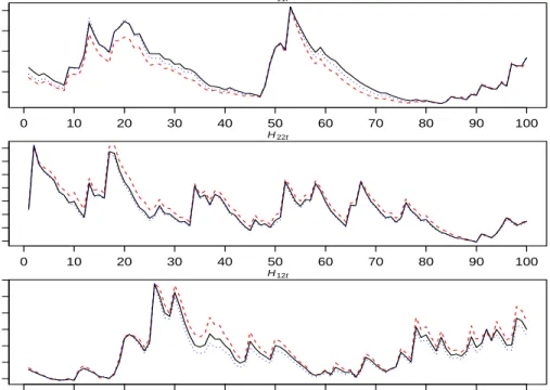
Finally, Figure 3 shows plots of volatilities and co-volatilities estimated under the assumption of skew student-t and standard normal errors against true values for a random sample of 100 observations when errors are gener-ated from skew student-t distribution. The plots show that using the skew
4900 4910 4920 4930 4940 4950 4960 4970 4980 4990 5000 1 2.5 4 H 11,t 4900 4910 4920 4930 4940 4950 4960 4970 4980 4990 5000 1 2.5 4 H 22,t 4900 4910 4920 4930 4940 4950 4960 4970 4980 4990 5000 0.3 0.6 0.9 R12,t
Figure 2: True (solid) and Bayesian (dashed-dot) estimates and 95% intervals (dotted) for volatilities Hii,t, fori= 1,2, and correlations R12,t,for the last 1000 observations for the simulated series of sample size T= 5000.
t model provides an improved performance from the normal model. The skew t model provides estimates remarkably close to the simulated volatili-ties, while at some points of time the difference between the two estimates is quite pronounced, e.g. H11,t at t = 20. In-sample maximum likelihood
estimates (MLEs) provided similar results, and hence they were not reported here. However, we favour here the MCMC approach as it provides more information of uncertainty quantification of the parameters subject to esti-mation.
H11t 0 10 20 30 40 50 60 70 80 90 100 4 6 8 10 H22t 0 10 20 30 40 50 60 70 80 90 100 4 12 20 28 H12t 0 10 20 30 40 50 60 70 80 90 100 2 3 4 5 6 7 8
Figure 3: Plots of Bayesian estimates of volatilities and co-volatilities estimated using skew student-t (dotted) and standard normal (dashed) errors against true (solid) values for a random 100 observations from the simulated series of sample sizeT= 2000 when errors are generated from skew student-t distribution.
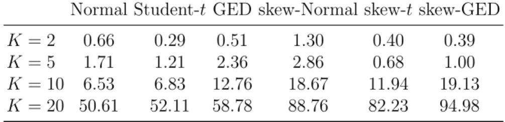
20 were also performed; for each simulated data set we have used 20000 it-erations for the MCMC. The accuracy of the estimates was not significantly affected by large dimensions, though greater computational cost was required to obtain the estimates, in particular regarding K = 20. Table 2 represents the computational time taken by an Intel Core i7 laptop with 16GB RAM for the estimation of RBEKK models. The code is written in the program-ming language R (https://www.r-project.org) with few routines in C++ language. Use of cluster and parallel computing are expected to improve computational time.
Table 2: Computational time (in minutes) taken by various RBEKK models forT = 1000.
Normal Student-t GED skew-Normal skew-t skew-GED
K = 2 0.66 0.29 0.51 1.30 0.40 0.39
K = 5 1.71 1.21 2.36 2.86 0.68 1.00
K = 10 6.53 6.83 12.76 18.67 11.94 19.13
K = 20 50.61 52.11 58.78 88.76 82.23 94.98
5
Empirical studies
In this section, we illustrate the proposed Bayesian approach using two real data sets.
5.1
DAX, CAC40 and NIKKEI indices
The first data set consists of the daily closing prices of the stock market indices in Frankfurt (DAX), Paris (CAC40), and Tokyo (NIKKEI) from Jan-uary 04, 2007 to October 31, 2018, a total of 2828 observations. This time period includes the global financial crisis of 2007-2008. The multivariate time series of de-meaned returnsri,t are defined as 100×{logPi,t−logPi,t−1},where
Pi,t is the daily closing price for stock i on day t. The skewness coefficients
for log-return series of DAX, CAC and NIKKEI are (0.1181,0.1111,−0.4940) whereas kurtosis are (10.3499,10.6778,10.8184). As we can see, all three return series have heavy-tails than the normal. The DAX and CAC40 log-returns are slightly positively skewed whereas the NIKKEI log-log-returns are found highly negatively skewed. Hence, we fit the diagonal RBEKK model
with heavy-tailed and skewed distributions for this data set.
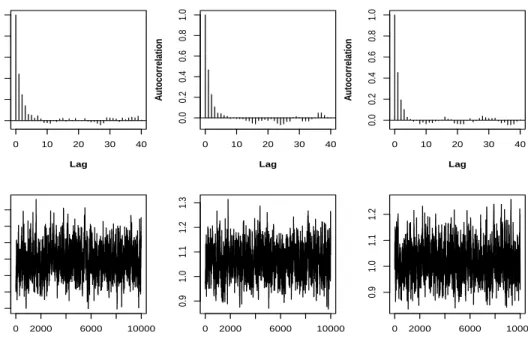
A Metropolis-Hastings algorithm with all the parameters updated as a block is adopted for the MCMC updates. A total of 20000 iterations are conducted with initial 10000 discarded in the burn-in stage. The simulated Markov chains were then checked for convergence and good mixing. Visual inspection of the marginal trace plots, density estimates and autocorrelation plots along with formal tests showed good convergence of the Markov chains. The autocorrelation and trace plots for the skewness parameter is shown in Figure 4. The trace plots seem to be stationary; this is evidenced visually by both the trace plots and the ACF plots. However, there seems to be some autocorrelation present. To minimise the effect of autocorrelation, thinning of 5 iterations is applied. Furthermore, we have initiated several chains and all had a similar effect. In addition to that running the chain for longer than 20000 iterations did not seem to have an effect and hence we do not report on longer chains. For this type of data we consider convergence as reasonable, although we do note some autocorrelation effect.
The deviance information criterion (DIC) and log marginal likelihood (LogML) are used to compare various models for the error terms (see e.g. Spiegelhalter et al., 2002, for a discussion). These include normal, skew normal, Student t, skewt, GED and skew GED. Note that smaller values of DIC and LogML are desired for a favourable model. The DIC is given by DIC = 2E[D(θM)]−D(E[θM]) whereD(·) is the deviance function defined as
0 10 20 30 40 0.0 0.2 0.4 0.6 0.8 1.0 Lag A utocorrelation γ1 0 10 20 30 40 0.0 0.2 0.4 0.6 0.8 1.0 Lag A utocorrelation γ2 0 10 20 30 40 0.0 0.2 0.4 0.6 0.8 1.0 Lag A utocorrelation γ3 0 2000 6000 10000 0.75 0.85 0.95 1.05 Iterations 0 2000 6000 10000 0.9 1.0 1.1 1.2 1.3 Iterations 0 2000 6000 10000 0.9 1.0 1.1 1.2 Iterations
Figure 4: Autocorrelation and trace plots for the skewness parameter.
modelM. To check whether the inclusion of skewness substantially improves the model fit, we calculate the weights associated with each DIC. The DIC weights are obtained as
wM ∝exp − DICM −DICB 2 ,
where DICB is the value associated with the ‘best’ model. The DIC weights
are then normalised to sum to 1. When the difference of DICM from DICB
is large (i.e. model M does poorly compared to the full model B) then the weight wM is small, while when DICM ≈ DICB, then the weight gets close
poste-rior distribution using non-parametric self-normalised importance sampling (Neddermeyer, 2009).
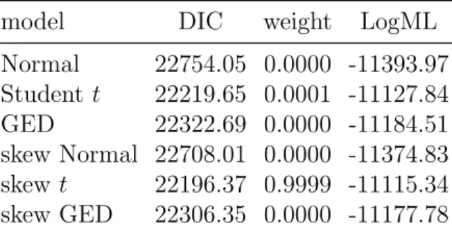
Table 3 below shows the DIC and LogML values for the diagonal RBEKK model, with six different innovation distributions, along with their weights. It can be seen that models with heavier tails exhibit a better behaviour than the normal distribution. Also note that skew distributions provide lower DIC and LogML values as compared to their symmetric versions. Moreover, the mul-tivariate skew t model is found to provide the best fit among the competing models. The DIC weight of this model is also found very large and far from all other models. The log marginal likelihoods of the RBEKK model with Studentt and skewtdistributions are, respectively, -11127.84 and -11115.34. This implies a Bayes factor of 2.7×10⁵ in favor of the RBEKK model with
skew t distribution, indicating overwhelming evidence of the latter. These findings indicate that incorporating the heavy tails with asymmetry in the error distribution provides a better fit for RBEKK model and consequently more precise volatilities and correlation estimates. Hence, in the sequel we report results for the multivariate skew t model only.
Table 4 presents the summary of the MCMC estimates of the diago-nal RBEKK model using a multivariate skew t distribution for the returns. Posterior means and standard deviations along with 95% credible intervals are displayed. The p-values of the convergence diagnostic (CD) of Geweke (1992) are also presented. For the Dax and NIKKEI log-returns, 95% credi-ble intervals for the skewness parameter do not include 1 and hence confirms
Table 3: DIC and LogML values and weights for various Diagonal RBEKK models.
model DIC weight LogML Normal 22754.05 0.0000 -11393.97 Student t 22219.65 0.0001 -11127.84 GED 22322.69 0.0000 -11184.51 skew Normal 22708.01 0.0000 -11374.83 skew t 22196.37 0.9999 -11115.34 skew GED 22306.35 0.0000 -11177.78
asymmetry in these series whereas estimates for skewness for CAC40 series are not found significant. The estimate of the tail parameter (ν) indicates the appropriateness of heavy tail of the distribution of the returns.
5.2
Portfolio allocation
In this section we discuss asset allocation, which is one of the main utili-ties and target applications of volatility estimation, in particularly regarding medium to high dimensional financial time series. Since parameter uncer-tainty largely affects the optimal asset allocation (Jorion, 1986), the Bayesian paradigm can offer an ideal estimation approach (see Kang, 2011, and Jacquier and Polson, 2013). We consider the global minimum variance (GMV) port-folio, with time-varying covariance matrices, which minimises the portfolio variance. Multivariate GARCH models were first used by Cecchetti et al. (1988) for optimal portfolio allocation and since then many studies have shown that using GARCH-type models reduce the portfolio risk (see Rossi and Zucca, 2002 and Yang and Allen, 2005, among others).
Table 4: MCMC estimates of the Diagonal RBEKK model with multivariate Skew t errors. Mean SD 95% interval CD DAX γ1 0.9011 0.0214 [0.8595, 0.9441] 0.6841 α11 0.0525 0.0061 [0.0412, 0.0657] 0.6518 β11 0.9328 0.0084 [0.9145, 0.9476] 0.9749 CAC40 γ2 0.9647 0.0254 [0.9175, 1.0157] 0.7397 α22 0.1108 0.0184 [0.0774, 0.1490] 0.9490 β22 0.8574 0.0252 [0.8034, 0.9025] 0.7353 NIKKEI γ3 0.9441 0.0223 [0.8988, 0.9862] 0.5103 α33 0.0594 0.0088 [0.0438, 0.0790] 0.5515 β33 0.9226 0.0123 [0.8947, 0.9432] 0.5809 ν 6.2094 0.3277 [5.6353, 6.8884] 0.9953
The posterior means are computed by averaging the simulated draws. SD is the standard deviation. The 95% intervals are calculated using the 2.5th and 97.5th percentiles of the simulated draws. Thep-values of convergence diagnostic statistic proposed by Geweke (1992) are reported under CD.
The one-step-ahead conditional covariance matrixHbT+1 is used to solve the portfolio allocation problem (see Yilmaz, 2011). The optimal portfolio weights for time T + 1 are obtained by solving the following optimization problem: w∗ = arg min w:w′1K=1Var[r ∗ T],
wherew= (w1, . . . , wK)′ is the weight vector, 1K is aK-vector of ones,r∗T = w′
rT is the portfolio return at timeT andrT is the vector of observed returns.
Without imposing short-scale constraint, i.e., wi ≥ 0,∀i = 1,2, . . . , K, the
w∗ T+1 = b H−1 T+11K 1′ KHb −1 T+11K . (10)
The proposed MCMC estimation enables us to approximate the posterior mean of the optimal portfolio weights as
E[w∗ T+1|rT]≈ 1 N N X n=1 w∗T(+1n), where w∗T(+1n) N n=1
is a posterior sample of the vector of optimal portfo-lio weights for each value of one-step-ahead conditional covariance matrix
b H(Tn+1)
N
n=1
in the MCMC sample. In this way, we solve the allocation problem at every MCMC iteration and obtain the approximate posterior mean of the optimal portfolio weights. The approximate posterior credible intervals for w∗
T+1 can also be obtained in by using the quantiles of the
sam-ple of optimal portfolio weights. Similarly, the optimal portfolio variance
σ2
w,T+1 =w ∗′
T+1HbT+1w∗T+1 can also be calculated and samples can be drawn
from its posterior distribution using MCMC.
In our approach uncertainty around the conditional volatility covariance matrix b H(Tn+1) N n=1
is passed onto uncertainty around the portfolio weights
and hence one can obtain a predictive sample σw2(,Tn)+1 (n = 1, . . . , N) of the
portfolio returns σ2
w,T+1. Following a more traditional approach, an investor
may obtain a point estimate ofHbT+1 (e.g. the mode ofHbT(n+1) ,n = 1, . . . , N)
forecast value of σ2
w,T+1. The two approaches should be equivalent for large
N, but our approach benefits by providing uncertainty around the volatility of the portfolio returns, which may be vital information for the investor. The mode of the forecast sample σw2(,Tn)+1 (n = 1, . . . , N) should provide a point
forecast of σ2
w,T+1, if this is needed.
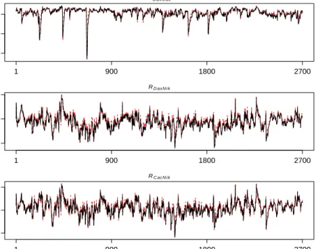
Bayesian estimates of conditional correlations when estimated with both skewtand Normal distributions for DAX, CAC40 and NIKKEI are presented in Figure 5. We observe that the correlation estimates of DAX and CAC40 largely agree over the two models: skew t and normal. However, for the correlation of DAX and NIKKEI and CAC40 and NIKKEI there appear to be some notable differences between the two models. We do not know the true correlations in the empirical studies, but the correlation estimates using the normal model appear to be more variable and less consistent for certain periods of time.
The first 2700 observations of DAX, CAC40 and NIKKEI data set are used for the estimation of the parameters of the RBEKK model with the skew t distribution and the remaining 128 observations (roughly six months data) are left for the out-of-sample forecasts. The forecast returns are ob-tained using a rolling window of size 2700 and the model is re-estimated each time a new observation vector is obtained (for the last 128 time points). This approach is appealing to practitioners and manages to capture the returns-dynamics better than in studies which the returns are estimated once from historical data, see e.g. Aguilar and West (2000). Figure 6
RD axC ac 0.5 0.7 0.9 1 900 1800 2700 RD axN i k −0.1 0.4 0.9 1 900 1800 2700 RC acN i k −0.2 0.3 0.8 1 900 1800 2700
Figure 5: Bayesian estimates of conditional correlations for DAX, CAX40 and NIKKEI index; Skew-t (solid) and Normal (dashed).
shows the log-returns of three stock indices for the out-of-sample period of
t = 2701, . . . ,2828.
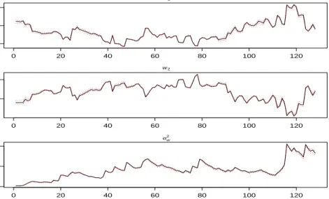
The optimal portfolio weights for the out-of-sample period are estimated. Figure 7 depicts the dynamics of the estimated portfolio weights and vari-ances along with their corresponding 95% credible intervals. The results of the first two portfolio weights w∗
i,T+1, i= 1,2 are reported as the third weight
can be obtained from these two.
Finally, to illustrate the proposed MCMC inference on a higher-dimensional data set, we use daily closing prices of eight stocks from the Dow Jones in-dustrial average (DJIA) index. The data set of 2242 observations is obtained from Yahoo!Finance for a sample period from January 02, 2001 to December 31, 2009. Noureldin et al. (2014) used the same data with ten stocks for the maximum likelihood estimation of RBEKK models assuming Gaussian distributions for the returns. In parallel to the earlier analysis, we split the data into two parts; the first 2100 observations are used for the estimation of the parameters of the model while the remaining 142 observation are used for out-of-sample forecasting. The diagonal RBEKK model is estimated us-ing both Bayesian and MLE methods assumus-ing a skew t distribution for the returns. The skew t distribution is chosen as its DIC value was found the lowest among other competing distributions. One-day-ahead forecasts of conditional covariance matrices are obtained and the GMV optimal portfolio without the short-scale constraint is constructed using both methods.
and MLE methods. For comparison purposes, cumulative portfolio returns using equal weights are also plotted in that figure. We remark that both cu-mulative returns (under the Bayesian and MLE estimation) outperform the equal weight allocation, which is very volatile and has a poor performance in the beginning and in the end of the sampling period. MCMC provides consistently better cumulative returns in comparison to the MLE, which is struggling to provide positive portfolio returns for about the first 60 trading days. If the assumed model is the true model, then the MLE is expected to at least as good as MCMC. We remark that the MLE algorithm took shorter time to run than MCMC, due to the large number of iterations required for the chains to reach convergence. The difference is more pronounced in higher dimensions. However, it is well known that maximum likelihood esti-mation for medium to high dimensional data can suffer from local maxima; the simulation study in Section 4 shows that the MCMC has the edge in pre-cision. Moreover, MCMC benefits by its capability of uncertainty analysis around the volatility estimates, the portfolio wights, the cumulative returns and associated expected risk and value-at-risk.
Figure 9 shows Bayesian and maximum likelihood estimates of portfolio variances for eight stocks of DJIA index. We remark that the variance perfor-mance of the portfolio between MCMC and MLE is similar (as both methods minimise the variance of the GMV portfolio). However, there are periods of time in which the portfolio variance under the skewt model is systematically smaller than the variance using the normal model, see e.g. t = 40−60 in
Figure 9.
6
Conclusions
In this article we have proposed Markov chain Monte Carlo estimation for a class of multivariate GARCH models for the estimation of volatility of fi-nancial returns. The proposed model benefits from covariance targeting and allows a parsimonious yet flexible treatment of asymmetry and heavy tails of the returns. In the core of the methodology there is a blocked Metropolis algorithm, which is shown to be efficient for small and medium dimensions in a simulation study. Volatility estimation on several assets and a port-folio study demonstrate the capabilities of the methodology. The proposed Bayesian estimation offers parameter uncertainty quantification, for exam-ple posterior summaries of volatilities, co-valatilities and dynamic correlation are provided. This is a useful consideration in assessing the uncertainty on portfolio returns, risk management and value-at-risk. As one referee has pointed out the model specification (1) proposed in Noureldin et al. (2014) can be generalised by replacing H1t/2 by a more general invertible matrix Z. Depending upon the structure of Z, the MCMC inference proposed in this paper may be extended to this interesting case.
The approach of covariance targeting may be applied to other GARCH-type models, such as the dynamic conditional correlation of Engle (2002), although further research should be conducted towards this direction. The
combination of covariance targeting and MCMC inference is a promising ap-proach, which we aim to explore in the near future for other multivariate volatility models.
Acknowledgements: The first author would like to thank Higher Ed-ucation Commission Pakistan for funding this research at the University of Sheffield, UK.
References
[1] Aguilar O, West M (2000) Bayesian dynamic factor models and portfolio allocation. Journal of Business and Economic Statistics 18: 338–357.
[2] Bauwens L, Laurent S (2005) A new class of multivariate skew densities, with application to generalized autoregressive conditional heteroscedas-ticity models. Journal of Business & Economic Statistics 23: 346–354.
[3] Bauwens L, Laurent S, Rombouts JVK (2006) Multivariate GARCH models: A survey. Journal of Applied Economics 21: 79–109.
[4] Bollerslev T, Engle RF, Wooldridge JM (1988) A capital asset pricing model with time-varying covariances. Journal of Political Economy 96: 116–131.
[5] Boswijk PH, van der Weide R (2011) Method of moments estimation of Go-GARCH models. Journal of Econometrics 163(1): 118–126.
[6] Braione M, Scholtes N (2016) Forecasting value-at-risk under different distributional assumptions. Econometrics, 4: 1–27.
[7] Cecchetti SG, Cumby RE, Figlewski S (1998) Estimation of the optimal futures hedge. Review of Economics and Statistics 70: 623–630.
[8] Chib S, Greenberg E (1995) Understanding the Metropolis-Hastings al-gorithm. The American Statistician 49: 327–335.
[9] Creal D (2012) A survey of sequential Monte Carlo methods for eco-nomics and finance. Econometric Reviews 31: 245–296.
[10] Engle RF (2002) Dynamic conditional correlation: a simple class of mul-tivariate generalized autoregressive conditional heteroskedasticity mod-els. Journal of Business Economics and Statistics 20: 339–350.
[11] Engle RF, Kroner KF (1995) Multivariate simultaneous generalized ARCH. Econometric Theory 11: 122–150.
[12] Fan J, Wang M, Yao Q (2008) Modelling multivariate volatilities via conditionally uncorrelated components. Journal of the Royal Statistical Society: Series B 70: 679–702.
[13] Fernandez C, Steel M (1988) On Bayesian modelling of fat tails and skewness. Journal of the American Statistical Association 93: 359–371.
[14] Fioruci JA, Ehlers RS, Filho, MGA (2014) Bayesian multivariate GARCH models with dynamic correlations and asymmetric error dis-tributions. Journal of Applied Statistics 41: 320–331.
[15] Geweke, J (1992) Evaluating the accuracy of sampling-based approaches to calculating posterior moments. In J.M.Bernardo, J.O.Berger, A.P. Dawid, & A.F.M. Smith (Eds.) Bayesian Statistics (Vol.4). Oxford: Clarendon Press.
[16] Jacquier E, Polson NG (2013) Asset allocation in finance: a Bayesian prespective. In: Demian P, Dellaportas P, Polson NG, Stephen DA (Eds.), Bayesian Theory and Applications, first ed. Oxford University Press, Oxford, pp. 501–516 (Chapter 25).
[17] Jorion P (1986) BayesStein estimation for portfolio analysis. Journal of Financial and Quantitative Analysis 21: 279–292.
[18] Kang L (2011) Asset allocation in a Bayesian copula-GARCH frame-work: an application to the passive funds versus active funds problem. Journal of Asset Management 12: 45–66.
[19] Neddermeyer, J (2009) Computationally efficient nonparametric impor-tance sampling. Journal of the American Statistical Association 104: 788–802.
[20] Noureldin D, Shephard N, Sheppard K (2014) Multivariate rotated ARCH models. Journal of Econometrics 179: 16–30.
[21] Osiewalski J, Pipien M (2004) Bayesian comparison of bivariate ARCH-type models for the main exchange rates in Poland. Journal of Econo-metrics 123: 371–391.
[22] Rossi E, Zucca C (2002) Hedging interest rate risk with multivariate GARCH. Applied Financial Economics 12: 241–251.
[23] Silvennoinen A, Ter¨asvirta T (2009) Multivariate GARCH modes. In T.G. Andersen, R.R. Davis, J.P. Kreiss, and T. Mikosch (Eds.). Hand-book of Financial Time Series 201–209. Springer-Verlag.
[24] Spiegelhalter DJ, Best NG, Carlin BP, Lindeven der A (2002) Bayesian measure of model complexity and fir (with discussion). Journal of the Royal Statistical Society: Series B 64: 1–34.
[25] van der Weide R (2002) Go-GARCH: a multivariate generalized orthog-onal GARCH model. Journal of Applied Econometrics 17: 549–564.
[26] Virbickaite A, Aus´ın MC, Galeano P (2015) Bayesian inference methods for univariate and multivariate GARCH models: a survey. Journal of Economic Surveys 29: 76–96.
[27] Vrontos ID, Dellaportas P, Politis DN (2003) A full-factor multivariate GARCH model. Econometrics Journal 6: 312–334.
[28] Yang W, Allen DE (2005) Multivariate GARCH hedge ratios and hedg-ing effectiveness in Australian futures markets. Accounthedg-ing and Finance 45: 301–321.
[29] Yilmaz T (2011) Improving portfolio optimization by DCC and DECO GARCH: evidence from Istanbul stock exchange. International Journal of Advanced Economics and Business Management 1: 81–92.
DAX −2.0 0.0 1.5 0 25 50 75 100 125 CAC −2.0 0.0 1.5 0 25 50 75 100 125 NIKKEI −3 0 2 0 25 50 75 100 125
Figure 6: Log-returns (in %) of DAX, CAC40 and NIKKEI index for t =
2701, . . . ,2828. w1 0 20 40 60 80 100 120 0.0 0.5 1.0 w2 0 20 40 60 80 100 120 0.3 0.8 σw2 0 20 40 60 80 100 120 0.4 0.8 1.2
Figure 7: A sequence of portfolio weights and variances along with their corre-sponding 95% intervals for t= 2701, . . . ,2828.
0 50 100 150 −10 −5 0 5 10 15
Figure 8: Out-of-sample cumulative portfolio returns for eight stocks of DJIA index; Bayesian (solid) and MLE (dashed) using the GMV portfolio. The equal weighted portfolio returns (dotted) are also displayed.
0.5
0.6
0.7
0.8
0 20 40 60 80 100 120 140
Figure 9: Out-of-sample portfolio variances for eights stocks of DJIA index; Bayesian (solid) and MLE (dashed).
![Table 4: MCMC estimates of the Diagonal RBEKK model with multivariate Skew t errors. Mean SD 95% interval CD DAX γ 1 0.9011 0.0214 [0.8595, 0.9441] 0.6841 α 11 0.0525 0.0061 [0.0412, 0.0657] 0.6518 β 11 0.9328 0.0084 [0.9145, 0.9476] 0.9749 CAC40 γ 2 0.964](https://thumb-us.123doks.com/thumbv2/123dok_us/9463185.2820953/25.918.165.750.239.561/table-mcmc-estimates-diagonal-rbekk-multivariate-errors-interval.webp)