Self-configuring data mining for ubiquitous computing

(1)

SELF-CONFIGURING DATA MINING FOR UBIQUITOUS COMPUTING

by

AYS¸EG ¨UL C¸ AYCI

Submitted to the Graduate School of Engineering and Natural Sciences in partial fulﬁllment of

the requirements for the degree of Doctor of Philosophy

Sabancı University January 2013

(2)

SELF-CONFIGURING DATA MINING FOR UBIQUITOUS COMPUTING

APPROVED BY

Assoc. Prof. Dr. Y¨ucel Saygın ... (Thesis Supervisor)

Assoc. Prof. Dr. Ernestina Menasalvas ...

Asst. Prof. Dr. G¨urdal Ertek ...

Assoc. Prof. Dr. Albert Levi ...

Assoc. Prof. Dr. Erkay Sava¸s ...

(3)

c

(4)

(5)

Acknowledgments

I would like to express my deepest gratitude to my supervisor Assoc. Prof. Dr. Y¨ucel Saygın, whose patience and kindness, as well as his academic experience, have been invaluable to me.

My sincere gratitude goes to Dr. Ernestina Menasalvas for her constant support during all the phases of my research. Her guidance helped me in all the time of research and writing of this thesis.

I thank Assoc. Prof. Dr. Albert Levi, Asst. Prof. Dr. G¨urdal Ertek, and Assoc. Prof. Dr. Erkay Sava¸s for their kind attendance to the thesis committee and for their valuable contributions.

Can Tunca and Engin Do˘gusay from Sabanci University contributed to this study by developing the supporting software. I thank them for their eﬀorts. Later on, Ahmet Can Kan from Sabanci University ported the supporting software to Android platform. I’m grateful to him for making the necessary changes to adapt the programs to Android platform in a very short time.

I also thank to my friends in Universidad Politecnica de Madrid: Dr. Santiago Eibe, Andrea Zanda, Jo˜ao Bartolo Gomes. I beneﬁted all the discussions we had done together.

Dr. ¨Ozlem C¸ etino˘glu provided me the formatting material for the thesis. Thanks for supporting me on formatting the thesis.

Finally, I am forever indebted to my son for his endless love, support, and patience. I am so lucky to have him.

(6)

SELF-CONFIGURING DATA MINING FOR UBIQUITOUS COMPUTING Ay¸seg¨ul C¸ aycı

Electronics Engineering and Computer Science Ph.D. Thesis, 2013

Thesis Supervisor: Assoc. Prof. Dr. Y¨ucel Saygın

Keywords: Data Mining, Ubiquitous Computing, Machine Learning

Abstract

Ubiquitous computing software needs to be autonomous so that essential decisions such as how to configure its particular execution are self-determined. Moreover, data mining serves an important role for ubiquitous computing by providing intelligence to several types of ubiquitous computing applications. Thus, automating ubiquitous data mining is also crucial. We focus on the problem of automatically configuring the execution of a ubiquitous data mining algorithm. In our solution, we generate configuration decisions in a resource-aware and context-aware manner. We propose to analyze the execution behavior of the data mining algorithm by mining its past executions. In order to extract the behavior model from algorithm’s executions, we make use of two different data mining methods which are Bayesian network and decision tree classifier.

Bayesian network is constructed in order to represent the probabilistic relationships among device’s resource usage, context, algorithm parameter settings and the perfor-mance of data mining.

Other data mining method that has been used is the decision tree classifier. The effects of resource and context states as well as parameter settings on the data mining quality are discovered through decision tree classifier. In this approach, a taxonomy is defined on data mining quality so that tradeoff between prediction accuracy and classification specificity of each behavior model that classifies by a different abstraction of quality, is scored for model selection.

We formally deﬁne the behavior model constituents, instantiate the approach for association rules and validate the feasibility of the two of the approaches by the exper-imentation.

(7)

MOB˙IL VER˙I MADENC˙IL˙I ˘G˙INDE OTOMAT˙IK YAPILANDIRMA Ay¸seg¨ul C¸ aycı

Elektronik M¨uhendisli˘gi ve Bilgisayar Bilimi Doktora Tezi, 2013

Tez Danı¸smanı: Do¸cent Dr. Y¨ucel Saygın

Anahtar Sözcükler: Veri Madencili˘gi, Mobil Sistemler, Makine Ö˘grenimi

¨

Ozet

Mobil cihazlarda kullanılan yazılımlar otonom olmalı ve kendilerini yapılandırmak gibi elzem kararları verebilmelidirler. Ayrıca, mobil platformlarda veri madencili˘ginin ¸ce¸sitli uygulamalarda daha akıllı kararlar almaları do˘grultusunda kullanılmaları ¨ onemli-dir. Dolayısıyla, mobil cihazlarda veri madencili˘ginin de otonom olması gereklidir. Bu tezde, mobil cihazlarda veri madencili˘gi algoritmalarını otomatik olarak yapılandırma konusunu ele aldık. Sunulan ¸cözümde, konfigürasyon önerileri üretilirken cihazın kay-naklarının kullanımı ve cihazın kullanıldı˘gı ba˘glam göz önüne alınmı¸stır ¸cünkü mobil cihazların kullanıldıkları ba˘glam sık¸ca de˘gi¸smektedir ve cihazın kaynakları da genel-likle kısıtlıdır. Veri madencili˘gi algoritmasının önceki ¸calı¸stırılı¸slarından i¸sleyi¸s mod-elinin ¸cıkarılarak yapılandırılmasında kullanılmasını önermekteyiz. Bu ama¸cla iki farklı yöntem denenmi¸stir: Bayesian network ve decision tree classifier.

Bayesian network kullanarak, cihaz kaynaklarının durumu, hangi ba˘glamda kul-lanıldı˘gı ile veri madencili˘gi yapılandırma de˘gerleri ve elde edilen performans arasındaki ili¸ski olasılıksal olarak g¨osterilmi¸stir. Bu bilgiye dayanarak, veri madencili˘gi uygula-masının ilerki ¸cali¸stırılı¸slarında mevcut duruma uygun yapılandırma kararları ¸cıkarıl-maktadır.

Veri madencili˘gi algoritmasının i¸sleyi¸s modelini ¸cıkarmakta kullandı˘gımız di˘ger y¨ on-tem ise decision tree classifier’dır. Cihaz kaynaklarının kullanım durumları ve cihazın hangi ba˘glamda kullanıldı˘gı ile algoritma yapılandırmasının elde edilen veri modeli kalitesine etkisi decision tree yöntemiyle sınıflandırma yapılarak ara¸stırılmı¸stır. Veri modeli kalitesi hiyerar¸sik olarak sınıflandırılmak suretiyle elde edilen olası veri maden-cili˘gi algoritması i¸sleyi¸s modellerinden en yüksek tahmin do˘grulu˘guna sahip olup aynı zamanda en özgül sınıflandırma yapan modeli se¸cmek i¸cin bir yöntem önerilmi¸stir.

Mobil cihazlarda ¸calı¸sacak bir veri madencili˘gi algoritması i¸sleyi¸s modelini olu¸sturan unsurlar tanımlanmı¸s, yöntem association rule mining algoritması i¸cin örneklenmi¸s ve yöntemin kullanabilirli˘gi deneysel olarak gösterilmi¸stir.

(8)

List of Figures

2.1 Overall view of automatic parameter setting . . . 8

4.1 Data mining conﬁguration using Bayesian network . . . 26

5.1 Data mining quality taxonomy speciﬁc to association rule mining . . . 33

6.1 Overall view of FESTweet . . . 50

7.1 Class descriptions of EDG . . . 53

7.2 Experiment phases . . . 55

7.3 Bayesian network of Apriori runs . . . 57

7.4 Main eﬀects plot of 4 quality measurements for home-short on memory 58 7.5 Assessment of recommendations derived from Bayesian network . . . . 62

7.6 Behavior model decay . . . 63

7.7 Cube of circumstances . . . 66

7.8 Data mining quality taxonomy used in the experiment . . . 68

7.9 Mappings from predecessor set domains to abstract domains . . . 70

7.10 Analysis of decision tree models . . . 71

7.11 Eﬀect of garbage classes on the model’s accuracy . . . 73

7.12 Assessment of recommendations derived from decision tree . . . 75

7.13 Processes for self-conﬁguring data mining . . . 78

8.1 Movie recommendations. . . 86

8.2 Eclipse DDMS . . . 90

(12)

C.1 Associations among movies . . . 108

C.2 Associations among movies (cont.) . . . 109

D.1 Subset of data collected by EDG . . . 111

E.1 Conﬁguration recommendations under possible circumstances . . . 113 E.2 Conﬁguration recommendations under possible circumstances (cont.) . 114

(13)

List of Tables

3.1 SampleC, P and Q . . . 22

5.1 Relation schema: discretized data mining quality . . . 32

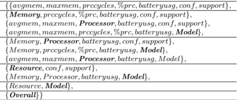
5.2 Lset: set of possible class label attribute sets . . . 35

7.1 Levels used for parameters . . . 56

7.2 Comparison of results . . . 60

7.3 Experiment fact table . . . 64

7.4 Attributes corresponding to symbols in taxonomy . . . 69

8.1 Parameters of Weka implementation of Apriori . . . 84

(14)

List of Abbreviations

P′ Conﬁguration of an algorithm

C′ Circumstance

Q′ Data Mining Quality

BS Bayesian Network Structure

P Relation schema for parameters

PI Set of parameter tuples

C Relation schema for circumstance

CI Set of circumstance tuples

Q Relation schema for quality features

QI Set of quality feature tuples

E Relation schema for execution data

EI Set of execution data

QD Relation schema for discretized quality features

QDI Set of discretized quality features

Qtuple _{Singleton set of quality features.} _Qtuple _⊆_Q DI

Qtuple_A Singleton set containing an aggregated quality feature

fA Aggregation function

QA Relation schema for aggregated data mining quality

QAI Set of tuples of aggregated data mining quality

QM Set of data mining attributes

QG Set of abstractions on data mining attributes

QT Set of data mining attributes and abstractions

(15)

Qgi Predecessor set of gi ∈ρ(QT) derived from taxonomy

Lset Set of class label attributes sets

G Relation schema for abstractions on quality

GI Set of quality abstraction tuples

fgi Mapping from predecessors set to their abstraction gi

Gtuple _{Singleton set of abstract quality features.} _Gtuple _⊆_G I

fALi Aggregation function to form i′th class label

QAL Relation schema for class labels of aggregated quality

QALI Set of class label tuples

Sset Screened set of class label attribute sets

QAS Relation schema for screened quality class labels

(16)

Chapter 1 INTRODUCTION

1.1 Motivation

Ubiquitous computing turned out to be today’s prominent computing paradigm as a result of the advances in related technologies, especially, wireless, mobile and sensor technologies coupled with the dissemination of these technologies in prices aﬀordable by large masses. Another important reason for the rise of this computing paradigm, is the availability of diverse application areas which beneﬁt ubiquitous computing. In a variety of ubiquitous computing applications such as ubiquitous health care systems, intelligent transportation systems and personal recommender systems, data mining is a preferred method for incorporating intelligence. Consequently, special consideration should be given to ubiquitous data mining which is complementary for a number of ubiquitous computing applications.

Ubiquitous computing deﬁnes an environment where resources for computing are spread rather than centralized and moreover, ubiquitous computing devices are oper-ated most of the time by individuals who are not computer savvy and even devices lie unattended in the environment. Data mining, on the other hand, is notorious for high demand of computing resources and often requires domain experts for tuning the process. Therefore, new principles and mechanisms for mining data on a platform con-sisting of restricted resource devices with versatile context where the expert interaction

(17)

is not available, are needed. In that respect, the essential features of a service provid-ing ubiquitous data minprovid-ing are resource and context-awareness as well as autonomous behavior and adaptability.

1.2 Approach

We address the problem of automatic conﬁguration of the execution of a data mining algorithm in a context and resource aware manner as a ﬁrst step towards deploying an autonomous ubiquitous data mining service that adapts to changing conditions. It is important to note that, autonomous behavior of a service is a broader concept which also involves decisions about scheduling the service, prioritizing its execution and others along with automatic parameter tuning.

Cao, Gorodetsky and Mitkas ([9]) discuss the contribution of data mining to agent intelligence. They argue that a combination of autonomous agents with data min-ing supplied knowledge provides adaptability whereas knowledge acquisition with data mining for adaptability relies on past data (past decisions, actions, and so on). Our approach to provide adaptability is similar: we use machine learning approach in order to generate adaptable parameter setting decisions and enhance ubiquitous data mining with autonomy and adaptability.

Following list summarizes the principles our approach:

• We propose to extract what we call the behavior model of a data mining al-gorithm’s execution for conﬁguring its parameters and we deﬁne formally what constitutes a behavior model in a ubiquitous computing environment.

• We present a solution that is based on learning from past experiences for fu-ture conﬁguration decisions which implies that the conﬁguration decisions can be adapted to changing conditions.

(18)

the proposed solution is not for a speciﬁc data mining algorithm.

• We propose a solution so that no restrictions are imposed on the types of the algo-rithm parameters when we configure by using the decision tree classifier. On the contrary, it is possible to configure continuous parameters as well as categorical.

• We analyze algorithm’s execution conditions against the quality of the acquired results. For the analysis, a combination of multiple quality indicators is consid-ered rather than individual ones and moreover the number of quality indicators may be extensive. Besides, behavior model classiﬁes execution data on various measurements of quality indicators. Thus, a single behavior model can be used for analysis of several performance criteria on a quality indicator.

1.3 Outline of the Thesis

The organization of this thesis is as follows:

Chapter 2 introduces the problem of automatically conﬁguring data mining in a ubiquitous computing environment while providing brief information on the methods used for the solution. Survey of related work is also provided.

In both of the approaches data collected during past executions of the data mining algorithm is used as the training set. In Chapter 3, we formally deﬁne the data model used in the approaches.

In Chapter 4 we present our approach to predict data mining algorithm behavior in ubiquitous computing environments using Bayesian Network.

The approach presented in Chapter 5 makes use of decision trees for the prediction of data mining algorithm behavior.

Instantiations of the approaches by making use of two motivating examples from the ubiquitous computing environment are given in Chapter 6.

(19)

Chapter 7 elaborates on the experimental evaluation of both of the approaches where the software designed and implemented for the experiments is also explained.

In Chapter 8, our approach is shown on mobile computing by making use of an Android device which runs one of the prominent mobile operating systems.

(20)

Chapter 2 PRELIMINARIES AND RELATED WORK

We present a mechanism to predict the appropriate settings of a data mining algorithm’s parameters in a resource-aware and context-aware manner. The mechanism is based on learning from past experiences, that is, learning from the past executions of the algorithm in order to improve the future decisions.

2.1 Analysis of the Problem

Our goal is to conﬁgure automatically a data mining algorithm which will run on a ubiquitous device. Since circumstantial factors such as the conditions of the resources and the context in which the device is used are important in a ubiquitous computing environment, availability of the knowledge on the following is useful for determining the algorithm’s appropriate conﬁguration:

• the resources that the algorithm needs in order to accomplish its task,

• the algorithm parameters that have an eﬀect on the resource usage or on the data model quality,

• the context features which may have an effect on the efficacy of the data mining model or the efficiency of data mining,

(21)

• the features of the mining data set,

• the quality indicators which show the eﬃcacy of the data mining model and eﬃciency of the data mining.

On the other hand, the problem that we tackle also implies the solution to address an important issue which is to change or improve the conﬁguration setting decisions as the circumstances change. That means that, automatically generated conﬁguration decisions must be adapted to the changing conditions just like a data miner expert who adapts his decisions when the conditions change.

Next, we deﬁne the factors for conﬁguration that we derive from the items outlined above

2.2 Problem Deﬁnition

When deciding how to set the parameters of an algorithm for a specific run, in a ubiquitous computing environment circumstantial factors (conditions of the device’s resources and the context in which the device is in) should be taken into account as well as the required quality. For this reason, we grouped the relevant factors for the configuration as circumstance and quality. Formal definition of automatic configuration of ubiquitous data mining problem is as follows:

C′: Circumstance is deﬁned by a set of ordered pairs (f,s) where f is either a resource or context feature and s is the state of this feature.

Q′: Quality is deﬁned by a set of ordered pairs (q,l) where q is a quality feature and l

is the required level for this quality. Quality features are metrics of eﬃciency or eﬃcacy of the algorithm.

P′: Parameter settings constituting the conﬁguration of the algorithm is deﬁned by a set of ordered pairs (p,v) where p stands for a parameter and v is the value it takes.

(22)

f: Let C′ and Q′ that are defined above, be the circumstance sensed and the required quality respectively, then automatic configuration for ubiquitous data mining which is defined as P′ above, is obtained by the mapping:

f :C′×Q′ →P′

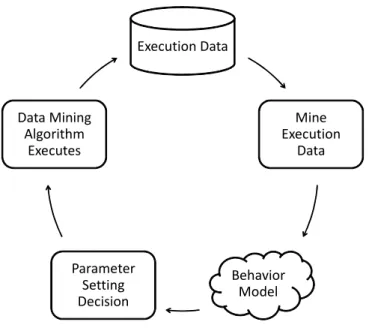
In this way, we covered all but the “features of the mining data set” outlined in problem analysis (subsection 2.1). We deliberately disregarded the effect of mining data set features on the configuration decision for the time being because we want to focus on the ubiquitous aspect in this work. On the other hand, we performed experiments to understand the effects of mining data set feature variation on the behavior model over time and discussed how to assess the deterioration of the behavior model performance. We propose to use data mining techniques to discover configuration of a data mining algorithm (P′), aiming to attain the requested quality (Q′), for the circumstance (C′) observed when a data mining request is issued. Our approach is to analyze the past behavior of algorithm under different circumstances and learn the appropriate config-uration(s) for data mining which satisfies the efficiency and efficacy requested. Thus a behavior model is created by mining data collected during past executions of the algorithm. Fig. 2.1 illustrates an overall view of the approach which consists of the following basic steps:

• Collect relevant information during the execution of the algorithm,

• Maintain a collection of past execution data,

• Learn a behavior model from the past execution data, and

• Use behavior model for automatic conﬁguration of data mining.

We proposed two approaches based on two data mining methods to solve self-conﬁguring data mining problem. Next, brief information on the data mining methods employed is given.

(23)

Execution Data Mine Execution Data Behavior Model Parameter Setting Decision Data Mining Algorithm Executes

Figure 2.1: Overall view of automatic parameter setting

2.3 Bayesian Networks

Bayesian networks which represent the joint probability distributions for a set of domain variables are proved to be useful as a method of reasoning in several research areas. Medical diagnosis([4]), language understanding ([17]), network fault detection([38]) and ecology([3]) are just a few of the diverse number of application areas where Bayesian network modeling is exploited. An in depth knowledge on Bayesian networks can be found in [53].

Classiﬁcation by using Bayesian networks is based on Bayes theorem which is given in Equation 2.1:

P(H|X) = P(X|H)P(H)

P(X) (2.1)

whereX and H is a pair of variables, P(X) and P(H) are theprobabilities ofX and

(24)

respectively.

A Bayesian network is a directed acyclic graph that shows the conditional depen-dencies between domain variables and may also be used to illustrate graphically the probabilistic causal relationships among domain variables. The nodes of the network represent the domain variables and an arc between two nodes (parent and child) indi-cates the existence of dependency among these two nodes. Conditional probabilities of the dependencies among each variable and its parents are also represented along with Bayesian networks. The joint probability of instantiated n variables (i.e. variable xi

has an assigned value) in a Bayesian network is computed by:

P(x1, ...., xn) = n

∏

i=1

P(xi|parents(Xi)) (2.2)

where parents(Xi) denotes the instantiated parents of the node of variable Xi.

Learning the Bayesian network structure rather than creating the structure by an-alyzing the dependencies of domain variables, is a ﬁeld of research which was studied extensively. Algorithms that learn the structure are most useful when there is a need to construct a complex network structure or when domain knowledge does not exist as in a ubiquitous computing environment. In depth information on topics of studies related to Bayesian networks can be found in [37] whereas a survey of literature on Bayesian networks is given in [8].

2.4 Decision Tree Classiﬁcation

Classiﬁcation by decision tree is inquiring the properties of an instance to ﬁnd out the class it belongs. For this purpose, a hierarchical structure named decision tree consisting of nodes and directed edges is used. Nodes of the tree correspond to the attributes of the instances whereas the leaf nodes constitute the class labels. Edges emanating from the non-leaf nodes are labeled by possible values or range of values of

(25)

the attribute represented by that node. It is possible to perceive each node as a test condition applied to an attribute and the edges from that node as the possible outcomes of the test.

A decision tree is built from a set of instances having preset class labels (training set) and then this structure is used to infer the unknown class labels of other instances which have the common attributes with the training set. A simple decision tree construction algorithm is to partition recursively the instances in the training set into smaller subsets by applying attribute test conditions one at a time until the class that the instances belong is found ([39]). Although the main logic of this algorithm is simple and it constitutes the basis of several decision tree algorithms, since the number of possible decision trees that can be generated from a given set of attributes is huge and moreover, some of the decision trees are more accurate than the others, successor algorithms were designed to construct a tree with reasonable accuracy without generating all the possible decision trees. While constructing a decision tree, giving precedence to the attributes that generate purer partitions with skewed class distribution is the preferred strategy. Entropy-based information gain, gini impurity and classiﬁcation error are three measures for calculating the impurity of an attribute. There are a number of well-known decision tree construction algorithms that make use of this strategy. ID3 [56], its extension C4.5 [57] and CART [6] are three important examples.

Due to the advantages this method possesses, decision tree classification has been used at various domains such as medicine for disease diagnosis, finance for fraud de-tection, credit approval and marketing to manage campaigns. Computational inexpen-siveness of decision tree construction can be counted as the foremost advantage as well as the fast classification that can be performed via a built decision tree. Furthermore, accuracy of decision tree is comparable to other classification methods and is preserved even there exist redundant attributes. Robustness to the presence of noise is yet another advantage. Decision trees are also favorable by being easy to interpret models.

(26)

2.4.1 Decision Tree Design Issues

The main objective of decision tree classiﬁcation is to minimize the classiﬁcation errors by avoiding the following:

• Training errors are incorrect classiﬁcations of training data. A possible cause is a training set where attribute combinations result in overlapping classes.

• Overﬁttingis high percentage of incorrect classiﬁcations of test data despite low training errors.

The following are among the most important issues that should be considered for gen-erating a good model for classiﬁcation.

• Dependent attributes. A model built by not taking into account the depen-dencies among the attributes of training data although related attributes exist.

• Nonpredictive attributes. Existence of a unique attribute such as a key or any attribute of training data that produces too many tiny partitions that is insuﬃcient for reliable classiﬁcation.

• Plethora of classes. The number of instances in the training set that pertain to a class is lower and less representative due to high number of diﬀerent classes.

2.5 Related Work

We attempt to solve the problem of ubiquitous data mining. In that respect, our work is related to existing study in ubiquitous data mining since we also consider the resource conditions and the context when generating the conﬁguration decisions similar to a number of studies in ubiquitous data mining. At the same time, our work bears similarities with automatic parameter conﬁguration which is a well searched area.

(27)

Hence, related work on both of the topics are given in separate subsections below. We ﬁnalize this section by discussing the diﬀerences among our work and others.

2.5.1 Ubiquitous Data Mining

Our focus in this work is ubiquitous data mining. Therefore, we determine the essential features of ubiquitous data mining considering the characteristics of the devices where the processing will take place. Consequently, when developing a data mining service for a ubiquitous device the following need to be taken into account:

• Resource-awareness

• Context-awareness

• Autonomous behavior

• Adaptability

In this subsection, we discuss our perspective and we mention the related work on ubiquitous data mining whereas our analysis of research challenge of ubiquitous data mining can be found in [12].

Resource and Context Awareness

Resource-awareness is assessing the availability of the required resources and reacting accordingly. The aim of resource-aware data mining service is to optimize the resource usage which necessitates knowing the necessary resources, being able to measure the availability of the device’s resources and knowing the eﬀects of the resources on its pro-cessing. Ubiquitous devices may have limited resources like processor power, memory and battery. Even if there is scarcity of a resource like memory, CPU or battery in the system, a data mining service may wisely switch to an alternative algorithm than the

(28)

desired one or alter its parameter settings to optimize the usage of the scarce resource and continue to service.

A number of studies has been proposed for ubiquitous data mining in resource constrained environments. Majority of these studies apply to data stream mining tech-niques. The approach in [27] [28] is for mining data streams where output granularity is adapted to the data rate of the stream, available memory and time constraints. In a later study ([30]), the idea of adapting output granularity is defined within a generic framework for resource aware stream mining where input rate and data mining al-gorithm are also adapted in a resource aware manner. A resource aware clustering algorithm for ubiquitous data streams is proposed in [16] where the algorithm settings are adapted and stream data is compressed based on available resources so that clus-tering with acceptable accuracy is possible even under constrained memory. A quality aware data stream mining model in [26] is able to adapt according to output quality as well as the resource consumption patterns. Succeeding work in [45] improves the former model by assessing the quality in real time. At a recent work, a general model of resource and quality aware data stream mining is proposed in [44] where its applica-bility is shown by the use of an example clustering algorithm. There are also resource aware stream mining solutions that apply only to specific algorithms. For instance, a frequent itemset stream mining algorithm is presented In [15] that utilizes an adaptive memory scheme to maximize the mining accuracy for confined memory space.

Context-awareness refers to the capability of sensing the environment and reacting accordingly. Context is domain/application specific most of the time but two common context features almost always used are location and time. In this work, we will refer to context-awareness in ubiquitous data mining as the capability of the device to adjust data mining preferences depending on circumstances in order to obtain better/more ac-curate results or improve the efficiency of the process. Context versatility of ubiquitous computing makes possible to fine tune data mining by considering the current context states. A number of examples are appropriate in order to give insight on how context can be used for ubiquitous data mining but certainly the usage is not restricted to these

(29)

examples. For example, time of day can be a criteria on determining the amount of mining such that more time consuming mining can be preferred during night. Context indicating the urgency of the situation that induces to use an already available model rather than re-generating the results is another example.

Similar to resource-aware solutions, context-aware ubiquitous data mining were also proposed for data stream mining. Context-aware stream mining was proposed by [33] where input and output granularity as well as algorithms of data stream mining are ad-justed dynamically and autonomously according to context. An approach for situation-aware adaptive processing of data streams was described in [34] and implementation for a health monitoring application was also shown. A domain speciﬁc context-aware ubiquitous stream mining model for intersection safety can be found in [58].

Autonomous and Adaptable Behavior

Autonomy and adaptability are two complementing features for a service. In general, autonomy is the ability of a service to determine independently what actions to take whereas adaptability is the ability to change the decision as the circumstances change. A ubiquitous data mining service behaves autonomously if whenever a mining re-quest is received; all the decisions about the mining process are taken independently by the service. Simply put, the decision is a set of actions to perform against the current situation. Setting a parameter value of data mining algorithm or selecting the appropriate input to mine are two examples of the actions. Context or availability of the resources which data mining service need may constitute a situation. The decisions in an adaptable ubiquitous data mining service, on the other hand, are dynamic and are expected to improve in terms of achieving the goals by learning from experience. Existent work on autonomous ubiquitous data mining focus on determining the pa-rameters of data mining algorithm either by statically binding situations (e.g., [29]) or dynamically determining the actions by correlation functions [34].

(30)

for self-conﬁguration of ubiquitous data mining aiming to fulﬁl the aforementioned requirements.

2.5.2 Automatic Parameter Conﬁguration

We propose a method to automatically determine the configuration of a data mining algorithm to execute in a ubiquitous computing device. Algorithm selection, config-uration setting or parameter tuning are similar research areas where similar solutions are proposed for the automatization. Present work on the automatization of either of them aims to speed up the process or to increase the probability of finding a solution to a specific problem instance. We emphasize automatic parameter tuning to provide autonomy in ubiquitous computing environments and it is important to use context and situation information when deciding and decisions need to be adaptive.

Taxonomy of varying approaches for solving the algorithm selection, configuration setting or parameter tuning problems is presented in several of the present research on algorithm selection, configuration setting and parameter tuning. Since existing tax-onomies are important resources for determining the lacking work of the research area, we provide a summary of the categories defined for automatizing algorithm selection/ configuration setting/parameter tuning by different authors before presenting our tax-onomy. In [40], three approaches are stated by taking into consideration the target problem. First approach they defined aims to find thebest default configuration across a set of given instances. Some of the mentioned related work of this approach involve racing algorithm, ILS search, fractional experiment design together with local search and decision tree classification. Second approach is defined as solving the algorithm selection problem which is selectingthe most appropriate algorithm given a problem in-stance. Usage of algorithm portfolios to choose among several algorithms is the general term where usage of empirical hardness model or case base reasoning are two example solutions given. Third approach in their categories is the online approach which is on-line in the sense that within a group of solutionsalternation between different problem solving strategies during execution is possible. In this approach tuning of parameters

(31)

and even algorithm selection decision is dynamically adjusted during execution. Ex-amples supplied that belong to that category employ a learning mechanism which is reinforcement learning most of the time, to improve the settings done and algorithm choice based on the information collected from the previous phases of the execution.

Another source of taxonomy for automatic parameter setting approaches is given in [52] where they distinguished the following approaches: evolutionary algorithm run, model selection and statistical estimation. In an evolutionary algorithm run which apply to evolutionary algorithms, programs and strategies, parameters are adapted during execution to obtain the best default conﬁguration. In model selection, optimization is performed based on a (usually) single objective to determine the best parameter setting among the existing models. Statistical approach is deﬁned as the estimation of the parameter setting using one of the estimation methods such as maximum likelihood (ML), expectation maximization (EM), maximum a posteriori (MAP) or hidden markov model (HMM).

In [31], the existent parameter tuning or algorithm selection techniques are dis-criminated using a number of orthogonal features: depending on the interval that tun-ing/selection is performed (performed once for a set of problem instances or repeated for each instance), whether the decision is made statically before execution or determined dynamically during execution and whether the learning technique is oﬄine (a separate training phase) or online (criteria is updated on every instance solution).

We distinguished two alternatives disciplines in the literature which are dominantly used to handle the parameter setting problem. These disciplines are (combinatorial) optimization methods and machine learning methods. Parameter tuning by optimiza-tion is a well searched area where proposed optimizaoptimiza-tions either tune parameters of a speciﬁc algorithm or provide optimizations to general cases.

Only a brief list of representative optimization solutions to parameter tuning is com-piled below as our work deviate a lot from them due to our preference of a machine learning technique for automatizing parameter tuning. The main idea behind

(32)

optimiza-tion is to determine performance criteria to be optimized and find the configuraoptimiza-tion that satisfies best this criteria. A racing algorithm by [5] for configuring metaheuristics, it-erated local search approach by [41] for configuration determination of an algorithm, a dynamic and online algorithm selection based on algorithm portfolios paradigm by [31], experimental design combined with local search to fine tune parameters of an algorithm by [1], are examples which employ an optimization technique.

Other prevailing technique proposed for automatic parameter tuning is based on machine learning classifiers. In general terms, classifiers are used to learn the parameters to set the configuration. In [59], usage of decision trees for automatic tuning of search algorithms is suggested. They describe both an online version where training data is not available and offline version in which training data is used for their method. In the offline version, a J48 decision tree using Weka is constructed to classify training data. The nodes of the tree are parameters of the algorithm, the branches from each node correspond to different values that parameter may take and the value on the leaf node classify the group of parameters as positive or negative with respect to a performance criteria. In their experiments runtime of the algorithm is used as the performance criteria. In order to derive candidate parameter settings, ranking functions are applied to the part of the decision tree which end to leaf nodes having positive values.

Bayesian networks are used by [52] to automatize the parameter tuning process. They distinguish two types of algorithm parameters as external and internal such that the former are the ones that must be tuned and the latter are established and updated in the model learning process. The “adjustment” model that they propose recommends values for the external parameters after the learning and inference phase. In the learning phase, Bayesian network is constructed from the data collected on previous runs. The domain variables are parameters of the algorithm and some eﬃciency measures. The inference mechanism updates the probability tables and obtains the most probable parameter values to obtain a “good” result from the algorithm.

In [51], the adjustment model is enhanced by a combined case-based reasoning system with the argument that optimal performance in diﬀerent problem domains is

(33)

attained by diﬀerent parameter settings. A case base which contains the Bayesian networks from the adjustment model and the characteristics of their associated problems is used for ﬁnding the similar problems of the domain. Similarities among problems are calculated using Euclidean distance function.

2.5.3 Characteristics Diﬀerentiating Our Approach

Existing resource-aware and/or context-aware adjustments of ubiquitous data mining parameters are proposed for data streams where data arrive continuously in a rapid speed. Hence, proposed solutions are specific to data stream mining and some are applicable to data stream mining algorithms with certain characteristics. On the other hand, we anticipated that all types of data mining will be required by ubiquitous computing applications. For example, mining multi-media data on the mobile device for the organization of music, picture and video files is one potential application area of ubiquitous data mining while data is not in streams ([47],[49]). Similarly, there are other prospective ubiquitous computing application areas such as user profiling ([32]), activity planning ([46]) and personal health monitoring ([19]) where there is a need to apply machine learning or mining techniques on data which is not streaming but batch. Thus, we worked on a general purpose solution to automatize the configuration of any data mining algorithm running on a ubiquitous computing environment without imposing any restrictions on the type of data mining algorithm or parameters.

The approach which we use for determining the configuration of data mining is also quite different from the work mentioned in the subsection 2.5.1 such that we employ data mining to discover the appropriate parameter settings from the history of execution results whereas proposed resource/context aware stream mining techniques do not use data mining methods to adjust stream mining parameters. The reasons we use a data mining technique for generating configuration decisions are twofold: to discover the effects of algorithm’s parameters to the quality of its results and to be able to adapt the configuration decisions to the changing conditions. In our solution, configuration decisions are adaptable in the sense that if there is a change on the discovered effects

(34)

due to a factor such as the growth of the data set which algorithm to be conﬁgured mines, new parameter to quality eﬀects can be tracked by regenerating or updating the behavior model.

Decision tree classiﬁers were suggested for automatic parameter setting like us in [59]. On the other hand, the method they suggested for automatically setting the parameters of an algorithm lacks being a general purpose solution due to following:

• Classiﬁcation can only be made on a single quality (performance) criteria. It is not possible to classify by combination of quality criteria.

• Diﬀerent parameter settings were classiﬁed into positive and negative examples with respect to a performance criteria which implies that only two levels of quality can be assessed.

• Assignment of class labels is static, quality attained after running the algorithm by the derived parameter settings is not used to correct the class labels.

• A new model would be needed when the performance criteria changes.

(35)

Chapter 3 DATA MODEL

Behavior model generation process uses data collected during past executions of the data mining algorithm in order to learn its behavior. In each execution of the algo-rithm, data specific to this run is captured and stored. This execution data is mined to construct behavior model. Since we have used execution data to construct Bayesian network and also to build decision tree, we formally define execution data before elab-orating on either of the approaches used for self-configuring data mining:

Deﬁnition 1 Let P(p1 : D1, ..., pn : Dn) be a relation schema deﬁning a data mining

algorithm’s parameters pi, where 1 ≤ i ≤ n. Let domi be the set of values associated

with the domain named Di.

An instance of P that satisﬁes the domain constraints is a set of tuples with n ﬁelds:

PI ={< p1 :d1, ..., pn:dn >|d1 ∈dom1, ..., dn∈domn}

Deﬁnition 2 Let C(c1 : D1, ..., cn : Dn) be a relation schema deﬁning context and

resource features (circumstance), ci, where 1 ≤ i ≤ n. Let domi be the set of values

associated with the domain named Di.

(36)

CI ={< c1 :d1, ..., cn :dn>|d1 ∈dom1, ..., dn∈domn}

Deﬁnition 3 Let Q(q1 :D1, ..., qn :Dn) be a relation schema deﬁning quality features,

qi, where 1 ≤ i ≤ n. Let domi be the set of values associated with the domain named

Di.

An instance of Q that satisﬁes the domain constraints is a set of tuples with n ﬁelds:

QI ={< q1 :d1, ..., qn :dn>|d1 ∈dom1, ..., dn ∈domn}

Deﬁnition 4 Let E(a1 :D1, ..., an :Dn) deﬁne a relation schema for execution related

data. An instance of execution dataE, namedEI, is the subset of the Cartesian product

(cross product) of the instances PI, CI, QI:

EI ⊂PI×CI×QI

In Table 3.1, sample relational schemas forC, P,andQtogether with small set of tuples as instantiations of each are given. For the given example, we assume that circumstance components (C) which may have an impact for the conﬁguration decision of data mining are location of the device and the time of day when the data mining is requested as well as the freememory in the device. A number of possible circumstances are sampled in the set CI such that each tuple in CI has a location, a time and a memory value

chosen fromldom,tdom andmdom respectively. We based our examples on association rule mining throughout the thesis for the coherence of explanations. On the other hand, we propose general guidelines for configuring any data mining algorithm. For this purpose, we exemplify in Table 3.1, k-means clustering as well as association rule mining as the data mining algorithms to be configured. We assume that association rule mining algorithm (ARM) that we configure has minimum support and minimum confidence parameters whereas number of clusters, maximum number of iterations and seed which is the number to be used for initial assignment of instances to clusters are the parameters of k-means. Memory usage (memusg) and the run time (duration)

(37)

Table 3.1: Sample C, P and Q

Relational Schema Domain

C ( location:ldom, ldom={indoor, outdoor} time:tdom, tdom={sunset, midday, night} memory:mdom) mdom={x|0< x≤M AXM EM} CI { < location:indoor, time:midday, memory: 500M >,

< location:outdoor, time:sunset, memory: 10K >,

< location:outdoor, time:night, memory: 1G > }

ARM P ( minsupp:sdom, sdom={x|0.3< x≤1}

minconf:cdom) cdom={x|0.6< x≤1}

PI { < minsupp: 0.5, minconf: 0.8>,

< minsupp: 0.5, minconf: 0.9>, < minsupp: 0.5, minconf: 0.95>,

< minsupp: 0.6, minconf: 0.7> } Q ( memusg:udom, udom={x|0< x≤M AXM EM}

duration:ddom, ddom={x|0< x≤1440}

model:odom) odom={strong, weak} QI { < memusg: 5K, duration: 10, model:strong >,

< memusg: 730K, duration: 3, model:weak >,

< memusg: 200M, duration: 125, model:strong > }

K-means P ( numClust:Cdom, Cdom={x|1< x≤30}

seed:edom) edom={10,15,20,25,30}

maxIter:idom) idom={x|1< x≤50}

PI { < numClust: 5, seed: 10, maxIter: 5>,

< numClust: 5, seed: 15, maxIter: 5>, < numClust: 5, seed: 20, maxIter: 5>,

< numClust: 6, seed: 15, maxIter: 5> } Q ( memusg:udom, udom={x|0< x≤M AXM EM}

duration:ddom, ddom={x|0< x≤1440}

W CSS:wdom) wdom={high, low} QI { < memusg: 5K, duration: 10, W CSS:high >,

< memusg: 730K, duration: 3, W CSS:low >,

(38)

of data mining are assumed to be the common quality metrics for both data mining. Interestingness degree of the model (model) and within-cluster sum of squares (WCSS) are the data mining quality metrics of ARM and k-means respectively.

(39)

Chapter 4 SELF-CONFIGURATION USING BAYESIAN

NETWORK

4.1 Behavior Model in the Form of Bayesian

Net-work

A Bayesian network is learned from the execution data and, afterwards, this Bayesian network representing the behavior model, is used to predict the appropriate conﬁgura-tions for the algorithm. Fig. 4.1 illustrates Bayesian network construction steps that we propose. K2 algorithm by [21] was used when constructing the Bayesian network. A comprehensive explanation of the method proposed in the papers [20],[21] can be found at Appendix A. Initial step of behavior model generation is to discretize the execution data since K2 assumes database variables to be discrete. K2 learns Bayesian network structure from database of cases (E in our case) by determining the most probable network structure Bs given E:

max

Bs

[P(Bs|E)] (4.1)

We made use of the open source code of Weka software ([35]) to construct the network and updated it to ﬁt our needs. The original algorithm seeks relationships among all the variables. However, execution data has three groups of variables (C,Q,P) and the relationships among the variables within a group such as the relationship among

(40)

circumstantial variables location and memory available are not interesting. For this reason, modification of the K2 algorithm is necessary to look for relationships among nodes belonging to different groups of variables. A level (lvl) is assigned to each group based on the possible cause-effect relationship between them. The levels are used to prevent the nodes in the lower level groups to be the parents of the nodes in the upper level groups. LetV={vl,k|l= 1, ..., lvlandk = 1, ..., xl}be the set of nodes of Bayesian

network where xl is the number of nodes in level l and vi,j, vm,n ∈ V. Then, i) nodes

vi,j and vm,n can not be related if i =m, ii) vi,j can be the immediate parent node of

vm,n only if m=i+ 1.

The Bayesian network that is constructed from past execution data represents the probabilistic relationship between circumstance states, discretized possible parameter settings, and measured as well as discretized quality indicators. Appropriate setting of an algorithm’s parameter is extracted from the Bayesian network as explained in the next section.

4.2 Mechanism to Predict Ubiquitous Data Mining

Conﬁguration

Once the behavior model is built, the steps that lead to automatic parameter conﬁgu-ration are as follows (See Fig. 4.1 for details):

• A data mining model is needed for a speciﬁc data set,

• Current circumstance (C′) is observed and the quality requirements (Q′) are ac-quired,

• Conﬁguration (P′) of the data mining algorithm is determined autonomously by inferencing from the behavior model

(41)

Categories of domain variables Evaluate current circumstance, required quality Bayesian network of circumstances, parameters and quality measurements Inference from Bayes network Circumstance, quality criteria ARM Request Configurate and run the algorithm Configuration •Circumstantial Information •Configuration Parameters •Quality Measurements Create execution record Execution record Group circumstantial, configuration, quality measures as nodes of the network Discretize Execution records Discretized records

Determine the level of each group Domain variables & groups CONSTRUCT BAYESIAN NETWORK Search relationship between nodes in all adjacent levels

(42)

The most likely conﬁguration is inferred from the behavior model by estimating the probabilities of possible parameter settings from previous runs of the algorithm in ex-ecution circumstances similar to current in order to obtain quality levels similar to the required. In particular,p(x|F) which is the conditional probability of x (an instantiation of parameter variable) given F (instantiations of circumstance and quality variables), is evaluated. Formal deﬁnition of inferring a value of a parameter from a Bayesian network structure is as follows:

Definition 5 ConsiderCI andQI defined in Definition 2 and Definition 3 respectively.

Let ctuple be any single tuple from CI and qtuple be the associated quality tuple from QI.

Consider the relation schema P(p1 : D1, ..., pn : Dn) that deﬁnes data mining

algo-rithm’s parameters(Deﬁnition 1). Let domi ={x1, x2, ...} be the domain set of pi. The

most likely setting of pi by a value from domi under the circumstance ctuple in order to

attain the data mining quality qtuple is the maximum of the φcalculated by:

(43)

Chapter 5 SELF-CONFIGURATION USING DECISION

TREES

5.1 Modeling the Behavior of a Data Mining

Algo-rithm with Classiﬁers

Predictive data mining is discovering from training data, patterns that can be gener-alized to forecast explicit values. Since, our approach for predicting future parameter settings is learning a model from past executions of the algorithm, we have chosen predictive data mining as the appropriate technique for discovering conﬁgurations.

Classification is a predictive data mining technique where a training set is used for discovering patterns to predict categorical values. We propose to use classification of execution data,E given in Definition 4 to create the behavior model of the data mining algorithm with the aim to use the model for predictive analysis of the algorithm’s behavior. Thus past execution data of the algorithm is used as the training data required for supervised learning of classification methods.

Eﬃciency of the data mining process and/or eﬃcacy of data mining model, which will be referred as data mining quality thereafter, are the objectives of parameter set-tings for a particular execution of a data mining algorithm. For that reason, we analyze

(44)

under diﬀerent circumstances the eﬀect of parameter settings on the data mining quality and thereupon we determine data mining quality as the class label to be predicted.

We will first elaborate on the properties of the class label chosen while discussing the necessary transformations and later explain in detail behavior model construction by using a specific classifier, decision tree. We have chosen decision trees classifiers due to the following reasons: i) Behavior model is constructed on a ubiquitous computing device where lowest resource consumption is essential. Existence of several computa-tionally inexpensive and fast decision tree construction algorithms makes decision tree classifier a suitable choice. ii) Data mining to be configured may have any kind of parameters. Decision trees can deal with continuous data as well as categorical data so that every kind of data mining parameters can be configured. iii) In general, accuracy of decision trees is comparable to other classification techniques. iv) It is possible to extract classification rules from decision trees which provide a convenient way to infer configurations.

5.1.1 Data Mining Quality as the Class Label

Since we have determined to use classiﬁers for solving automatic parameter setting problem, data mining quality attributes (each qi in Deﬁnition 3) are converted to

cate-gorical attributes. Formal deﬁnition of discretized data mining quality Qis as follows:

Deﬁnition 6 Let QD(q1 : D1, ..., qn : Dn) be a relation schema deﬁning quality

fea-tures, qi, where1≤i≤n. Let domi be the set of pairs (l, u) associated with the domain

named Di such that each pair corresponds to the lower and upper boundaries of a bin

interval after discretization.

An instance of QD that satisﬁes the domain constraints is a set of tuples with n ﬁelds:

(45)

In order to use data mining quality as the class label of the classiﬁer, Q given in Deﬁnition 6 is converted to a unary relation having a single attribute (sayqA). Next, we

deﬁne the aggregation function to derive aggregated data mining quality. The aggrega-tion funcaggrega-tion,fA that will be used for this purpose may consist of arbitrary operations

given that a single value, qA is obtained by making use of all other quality attributes

q1, , qn and fA should be an invertible function so that q1, , qn could be re-generated

given qA:

Deﬁnition 7 Let Qtuple _{be a set containing any single tuple from} _Q

DI. Let Q

tuple A be

a singleton set containing a unary tuple. Aggregation function for data mining quality,

fA is an invertible function that deﬁnes the mapping from Qtuple to QtupleA given as:

fA :Qtuple −→Q tuple A

Finally, formal deﬁnition of aggregated data mining quality is as follows:

Deﬁnition 8 Let QA(qA : DA) deﬁne a relation schema for aggregated data mining

quality and domA=RfA is the set of values associated with the domain named DA.

An instance of aggregated data mining quality, QAthat satisﬁes the domain constraints

is a set of tuples with 1 ﬁeld:

QAI ={< qA :dA>|dA∈domA}

5.2 Predicting the Behavior of a Data Mining

Al-gorithm with Decision Trees

We propose to use decision tree classifier to obtain a model that maps the attribute sets consisting of circumstance (Definition 2) and parameters (Definition 1) to the class

(46)

label aggregated data mining quality (Deﬁnition 8):

f :C×P −→QA

Since aggregated data mining quality (QA) is a composite attribute formed by

ag-gregation of a number of attributes, the number of possible data mining quality classes is denoted with the following equation:

κ=

n

∏

i=1

ki (5.1)

wherenis the number of attributes inQD, andkiis the cardinality ofith attribute’s

domain (number of bins).

Although classifying byQAwill provide classes with exact data mining quality

infor-mation, the resulting number of aggregated quality classes (given in equation 5.1) can be too high preventing accurate classification. For this reason, we consider abstractions of QA as well as QA as possible class label attributes. We aim to find a tradeoff

be-tween estimated accuracy and classification specificity by ranking the possible behavior models that can be generated using different abstractions of data mining quality as the class label attribute.

5.2.1 Abstractions over the Class Label

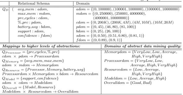
We consider diﬀerent abstraction levels of data mining quality as possible class labels. A hierarchical structure that shows the taxonomy of data mining quality attributes in

QD is used to abstract the data mining quality:

Deﬁnition 9 Data mining quality abstraction is composed of:

• A tree structure T representing data mining quality taxonomy where QT is the

(47)

Table 5.1: Relation schema: discretized data mining quality

Relational Schema Domain

QD ( avg mem:adom, adom={(0,100000),(100001,1000000),(1000001,10000000)

max mem:mdom, mdom={(0,250000),(250001,4000000), prc cycles:cdom, (4000001,10000000)}

%prc:pdom, cdom={(0,200K),(200K,4M),(4M,10M),(10M,20M)

battery usg:bdom, pdom={(0,45),(46,80),(81,100)}

support:sdom, bdom={(0,25),(26,100)}

conf idence:f dom) sdom={(0,0.50),(0.51,0.80),(0.81,1)}

f dom={(0,0.89),(0.9,1)}

Mappings to higher levels of abstractions: Domains of abstract data mining quality:

QP rocessor={prc cycles,%prc} M emorydom={V eryLow, Low, Average,

cdom × pdom→P rocessordom High, V eryHigh} QM emory={avg mem, max mem} P rocessordom={V eryLow, Low,

adom × mdom→M emorydom Average, High, V eryHigh} QResource={P rocessor, M emory, battery usg} Resourcedom={Low, Average,

P rocessordom×M emorydom×bdom→Resourcedom High, V eryHigh} QM odel={support, conf idence} M odeldom={Low, Average, High}

sdom × cdom→M odeldom Overalldom={Good, Bad} QOverall={M odel, Resource}

M odeldom × Resourcedom→Overalldom

QG={g1, g2, ...}=QT −QD be the set of abstract data mining quality attributes.

QG is partially ordered such that a quality attribute in QG comes before its parent

in T.

• Domain sets gidom of each gi ∈QG.

• Stepwise mappings to higher abstract levels. For each gi ∈QG where i= 1, ...,|QG |:

– Let Qgi be the successor set of gi in T.

– Every combination of elements from the domain sets of Qgi is mapped to the

domain values of gi such that:

fgi :q1dom×q2dom×....×q|Q_gi|dom→gidom

where qidom is the domain set of i′th member of Qgi.

Data mining quality abstraction given in Deﬁnition 9 is explained by the following example. Discretized data mining quality schema, QD in Table 5.1 is used in the

ex-ample to deﬁne usage measurements of device’s resources such as memory (avg mem, max mem), processor (prc cycles,% prc) and battery(battery usg) by the data min-ing process as well as the calculations obtained from the data minmin-ing model such as

(48)

Resource

Overall

Model

Memory Processor battery_usg support confidence

avg_mem max_mem prc_cycles %_prc

Figure 5.1: Data mining quality taxonomy speciﬁc to association rule mining

conf idence and support. Figure 5.1 is the data mining quality taxonomy where the leaf nodes are the “actual” data mining quality features (QD) whereas interior nodes

are the quality abstractions (QG).

The domains (gidom) of abstract data mining quality features which are the

gen-eralizations of the Memory, Processor and Resource usage as well as the data mining

Model and Overall quality are shown in Table 5.1. Successor sets of abstract data min-ing quality features (QP rocessor, QM emory and so on) are derived from the taxonomy T

according to Deﬁnition 9. The values of the features in its successor set determine the value of abstract feature. For this reason, each combination of values from the domains of the features in the successor set of an abstract feature is mapped to a value in its domain. For example, when average memory usage and maximum memory usage are in the range(0,100000) and (250001,4000000) respectively, then Memory usage of the process isAverage, is a possible mapping that gives the value of an abstract data min-ing quality feature based on the quality features in its successor set. The appearance order of successor sets in Table 5.1 follow the partial order that is determined from the taxonomyT.

Self-configuring data mining for ubiquitous computing

Acknowledgments

Abstract

¨

Ozet

Contents

List of Figures

List of Tables

List of Abbreviations

Chapter 1

INTRODUCTION

1.1

Motivation

1.2

Approach

1.3

Outline of the Thesis

Chapter 2

PRELIMINARIES AND RELATED WORK

2.1

Analysis of the Problem

2.2

Problem Deﬁnition

2.3

Bayesian Networks

2.4

Decision Tree Classiﬁcation

2.4.1

Decision Tree Design Issues

2.5

Related Work

2.5.1

Ubiquitous Data Mining

2.5.2

Automatic Parameter Conﬁguration

2.5.3

Characteristics Diﬀerentiating Our Approach

Chapter 3

DATA MODEL

Chapter 4

SELF-CONFIGURATION USING BAYESIAN

NETWORK

4.1

Behavior Model in the Form of Bayesian

Net-work

4.2

Mechanism to Predict Ubiquitous Data Mining

Conﬁguration

Chapter 5

SELF-CONFIGURATION USING DECISION

TREES

5.1

Modeling the Behavior of a Data Mining

Algo-rithm with Classiﬁers

5.1.1

Data Mining Quality as the Class Label

5.2

Predicting the Behavior of a Data Mining

Al-gorithm with Decision Trees

5.2.1

Abstractions over the Class Label