Targeted Minimum Loss Based Estimator that Outperforms a given Estimator

University of California, Berkeley

U.C. Berkeley Division of Biostatistics Working Paper Series

Year  Paper

Targeted Minimum Loss Based Estimator that

Outperforms a given Estimator

Susan Gruber

Mark J. van der Laan

∗_{University of California, Berkeley, [email protected]} †_{University of California - Berkeley, [email protected]}

This working paper is hosted by The Berkeley Electronic Press (bepress) and may not be commer-cially reproduced without the permission of the copyright holder.

http://biostats.bepress.com/ucbbiostat/paper280 Copyright c2011 by the authors.

Targeted Minimum Loss Based Estimator that

Outperforms a given Estimator

Susan Gruber and Mark J. van der Laan

Abstract

Targeted minimum loss based estimation (TMLE) provides a template for the con-struction of semiparametric locally efficient double robust substitution estimators of the target parameter of the data generating distribution in a semiparametric censored data or causal inference model (van der Laan and Rubin (2006),van der Laan (2008), van der Laan and Rose (2011)). In this article we demonstrate how to construct a TMLE that also satisfies the property that it is at least as efficient as a user supplied asymptotically linear estimator. For the sake of illustration we focus on estimation of the additive average causal effect of a point treatment on an outcome, adjusting for baseline covariates.

1

Introduction

Targeted minimum loss based estimation (TMLE) provides a template for the con-struction of semiparametric locally efficient double robust substitution estimators of the target parameter of the data generating distribution in a semiparametric cen-sored data or causal inference model (van der Laan and Rubin (2006); van der Laan (2008); van der Laan and Rose (2011)). It is assumed that the data set is a realiza-tion ofn independent and identically distributed random variables, the probability distribution of this random variable is known to be an element of a semiparamet-ric statistical model, and the target parameter (mapping) is defined as a particular function of the possible probability distributions in this semiparametric model. A targeted minimum loss based estimator (TMLE) of the target parameter is defined by an initial estimator of a relevant part of the data generating distribution, a para-metric submodel through an initial estimator, a loss function for this relevant part, minimizing the empirical risk of the loss function along the parametric submodel to iteratively update the initial estimator until convergence. This final estimator is the TMLE of the relevant part of the data generating distribution, and the evaluation of its target parameter value is the TMLE of the target parameter. By enforcing that the loss-based score of the submodel (at zero fluctuation of the initial esti-mator) spans the efficient influence curve of the target parameter (at the initial estimator), it follows that the TMLE of the relevant part of the data generating distribution solves the efficient score estimating equation, making the TMLE locally efficient and double robust, under regularity conditions. By choosing a parametric submodel with extra fluctuation parameters, the TMLE can be arranged to solve additional estimating equations, and thereby satisfy additional properties of inter-est (e.g., be an imputation inter-estimator, see Gruber and van der Laan (2010a)). One particular example of such an iterative TMLE was presented in the original TMLE article, van der Laan and Rubin (2006), which involved also fluctuating the treat-ment/censoring mechanism, resulting in a TMLE that also equals an IPTW/IPCW estimator and is guaranteed to outperform the IPTW/IPCW estimator defined by the initial estimator of the treatment/censoring mechanism.

Another property of interest of an estimator is that it is guaranteed to be more efficient than a user supplied class of estimators in the case that the cen-soring/treatment mechanism is correctly specified. This has been achieved with empirical efficiency maximization (Rubin and van der Laan (2008), Tan (2008),Cao et al. (2009),van der Laan and Rose (2011)). However, in general this technique as presented in Rubin and van der Laan (2008) may come at a cost of losing double robustness (e.g, see Robins and Rotnitzky (1992), van der Laan and Robins (2003). Tan (2008) demonstrates how in the context of estimating equation methodology the double robustness can be preserved. Recently, Rotnitzky et al. (2011) shows how to combine empirical efficiency maximization with double robust locally efficient substitution estimators, by fluctuating the treatment mechanism with a carefully

chosen clever covariate derived from the empirical efficiency maximization proce-dure. Borrowing this fundamental idea, in this article we demonstrate that this enhanced efficiency property can be achieved with the above mentioned TMLE of van der Laan and Rubin (2006) (jointly updating treatment mechanism and out-come regression), by fluctuating the treatment mechanism with this additional clever covariate as suggested by Rotnitzky et al. (2011). For the sake of illustration we focus on estimation of the additive average causal effect of a point treatment on an outcome, adjusting for baseline covariates.

1.1 Organization

In Section 2 we present the statistical estimation problem. In Section 3 we present the TMLE, and the enhanced empirically efficient TMLE, and explain its properties. From the presentation in Section 3, for experts familiar with the theory of augmented IPCW estimating equations (Robins and Rotnitzky (1992), van der Laan and Robins (2003)) it will also be clear how this TMLE is generalized to all CAR-censored data and causal inference models. In Section 4 we review the method for empirical efficiency maximization of Rubin and van der Laan (2008), and an adaptive version of it as presented in van der Laan and Rose (2011), used as an ingredient in the enhanced empirically efficient TMLE. In Section 5 we present simulations confirming the enhanced efficiency property of the TMLE presented in Section 3, and comparing it with the (non-double robust) empirical efficiency maximization estimator in Rubin and van der Laan (2008), and a regular TMLE. We end with some concluding remarks. We also provide an appendix with the R-code of the TMLEs implemented in the simulation study.

2

The statistical model, target parameter, and

estima-tion problem

Let O = (W, A, Y) ∼ P0 be a random variable, where W represents a vector of

baseline covariates, A a binary treatment, and Y a continuous or binary outcome with values in [0,1]. Let g0(A | W) be the conditional probability distribution of A, given W. Consider a statistical model M that makes no assumptions about the marginal distribution of W, and the conditional distribution ofY, given A, W, but might make assumptions about g0. In particular, it is assumed that 0< g0(1| W)<1 so that the following target parameter is well defined. The statistical target parameter Ψ :M →IR of interest is defined as

Ψ(P) =EP(EP(Y |A= 1, W)−EP(Y |A= 0, W)).

If one assumes an underlying nonparametric structural equation modelW =fW(UW),

A=fA(W, UA),Y =fY(W, A, UY) (Pearl (2000)), and the randomization

effectE0(Y(1)−Y(0)), where Y(a) =fY(W, a, UY) is the treatment-specific coun-terfactual. For the sake of estimation, we are only concerned with the statistical target parameter.

Let QW(P) be the marginal distribution of W under P, ¯Q(P)(A, W) =EP(Y |

A, W), and we will denote corresponding parameter values withQW and ¯Q, respec-tively. Let Q(P) = (QW(P),Q¯(P)). Note that Ψ(P) only depends on P through

QW(P) and ¯Q(P). Therefore, we will also use the notation Ψ(Q) =EQW{Q¯(1, W)−Q¯(0, W)}.

Our goal is to estimateψ0 = Ψ(Q0) based on observing ni.i.d. copiesO1, . . . , On of

O∼P0 ∈ M.

The TMLE requires knowing the canonical gradient/efficient influence curve of the pathwise derivative of Ψ :M →IR. The efficient influence curve of Ψ :M →IR atP is given by D∗(P)(O) = 2A−1 g(A|W)(Y −Q¯(A, W)) + _¯ Q(1, W)−Q¯(0, W)−Ψ(Q) ≡ D_Y∗(P)(O) +D_W∗ (P)(W),

where the latter decomposition in a scoreD∗_Y(P) of the conditional distribution of

Y, givenA, W, and scoreD∗_W(P) of the marginal distribution ofW will be utilized in TMLE. In order to establish the enhanced efficiency property of the proposed TMLE we will also utilize the augmented IPCW-representation of the efficient influence curve (Robins and Rotnitzky (1992), van der Laan and Robins (2003)):

D∗(P)(O) = 2A−1 g(A|W)Y −Ψ(Q)− ¯ Q(1, W) g(1|W) + ¯ Q(0, W) g(0|W) (A−g(1|W)) ≡ DIP T W(Q, g)(O) +DCAR( ¯Q, g)(O), whereDCAR( ¯Q, g) =−HCAR(Q, g)(W)(A−g(1|W)) with

HCAR(Q, g)(W)≡ ¯ Q(1, W) g(1|W) + ¯ Q(0, W) g(0|W) .

In cases where we want to stress the representation of the efficient influence curve

D∗(P) as an estimating function in ψ indexed by nuisance parameters ¯Q0, g0, we will also use the notationDIP T W(ψ0, g0) forDIP T W(Q0, g0), andD∗(ψ0,Q¯0, g0) for D∗(P0).

Another ingredient of the TMLE presented in the next section is an influence curve D(P) of a competing regular asymptotically linear estimator of Ψ at P in the model M. The TMLE ψ_n∗ will be constructed so that it is at least as efficient as this competing estimator at P0 in the case that we estimate g0 consistently. By

the representation theorem for the class of gradients in CAR-censored data models (van der Laan and Robins (2003), p. 65), it follows that

D(P) =DIP T W(Q, g) +DCAR( ¯Qe, g)

for a particular function ¯Qe= ¯Qe(P). Let ¯Qe₀denote the true value of this parameter

P →Q¯e(P).

The TMLE presented in the next section will use an estimator ¯Qe_n of ¯Qe₀ in order to define a clever covariateHCAR( ¯Qe_n, gk_n) in the definition of the TMLE. As a consequence of this choice of clever covariate, the TMLE Q∗_n, g_n∗ will solve

0 =PnDIP T W(ψ∗n, gn∗) +DCAR( ¯Qen, gn∗),

and thereby have an influence curve at least as efficient as D(P0), ifg0 is estimated consistently.

A particular choice of interest for ¯Qe

0is defined by empirical efficiency maximiza-tion over a user-supplied working model as in Rubin and van der Laan (2008). That is, let {Q¯β :β} be a parametric working model, and define

¯

Qe(P0) = arg min ¯ Qβ

P0{DIP T W(ψ0, g0) +DCAR( ¯Qβ, g0)}2. (1)

Here we used the notation P f ≡ R

f(o)dP(o). With this choice, D(P0) repre-sents the influence curve with minimal variance among the class of influence curves

{DIP T W(Q0, g0) +DCAR( ¯Qβ, g0) :β} indexed byβ.

3

The TMLE that is at least as efficient as competing

estimator

The TMLE of Ψ(Q0) as presented in van der Laan and Rubin (2006) is defined by 1) a loss functionL(Q, g) =L(Q) +L(g) for (Q0, g0) so thatQ0= arg minQP0L(Q), g0 = arg mingP0L(g), 2) a submodel {Q(1) :1} through Q at1 = 0, a submodel

{g(2) :2} through g at2 = 0, and 3) an initial estimator Q0n, g0n. The TMLE is defined by iterative minimization of the empirical risk, and updating:

1n = arg min 1 PnL(Q0n(1)) 2n = arg min 2 PnL(g0n(2)),

Q_n1 = Q0_n(1n), gn1 = g0n(2n), and this updating process is iterated till n = (1n, 2n)≈0. The resultingQ∗n, gn∗ solve the loss-based score equation:

Pn d dL(Q ∗ n(), gn∗()) =0 = 0. (2)

By defining the loss-function L and submodel through (Q, g), one can control the estimating equation (2) the TMLE solves. In particular, one wants the loss-based scores to span the efficient influence curve D∗(Q∗_n, g_n∗) so that the resulting Ψ(Q∗_n) will be double robust and locally efficient. Below we present a submodel{g(2) :2} so that the additional desired enhanced efficiency property is achieved as well.

3.1 Initial estimators

LetQ0_W,n, ¯Q0_n,g_n0, and ¯Q_ne be initial estimators ofQW,0, ¯Q0,g0, and ¯Qe0, respectively. Let Q0_W,n = QW,n be the empirical probability distribution of W1, . . . , Wn. The estimator of ¯Q0 can be based on the least squares or (quasi-)log-likelihood loss function

L( ¯Q)(O) =−

Y log ¯Q(A, W) + (1−Y) log{1−Q¯(A, W)} . (3) This is the log-likelihood loss-function for ¯Q0 if Y is binary. We refer to Gruber and van der Laan (2010b) in which this loss function is proposed for TMLE with a continuous bounded outcome Y ∈ [0,1]. By a simple linear transformation, this also provides a loss function for Y ∈ [a, b] with bounded a, b. In particular, ¯Q0 could be estimated with a loss-based super learner using this loss function for the cross-validation selector (van der Laan et al. (2007)).

The estimator of g0 can be based on the log-likelihood loss function L(g) =

−logg. The estimation method for ¯Qe₀ might depend on the type of parameter it represents. If ¯Qe₀ is defined by (1), then one could estimate it as

¯

Qe_n= arg min ¯ Qβ

Pn{DIP T W(ψ0n, gn0) +DCAR( ¯Qβ, gn0)}2, (4) wherePn denotes the empirical probability distribution ofO1, . . . , On, and ψ0n rep-resents an estimator of ψ0 that is consistent if gn0 is consistent. For example, ψ0n could be any TMLE that takes ¯Q0_n andg_n0 as initial estimator. We assume that ¯Qe_n

is consistent for ¯Qe₀ ifg0_n is consistent.

3.2 Loss function

We select the log-likelihood loss functions L(g) = −logg, L(QW) = −logQW for

g0 and QW,0, respectively, and we select L( ¯Q) (3) as loss function for ¯Q0. Let L(Q, g)≡L( ¯Q) +L(QW) +L(g) be the loss function for (Q0, g0).

3.3 TMLE that is at least as efficient as competing estimator

Let ¯g(W)≡g(1|W). For a given ¯Qk_n,g_nk, define the submodels Logit ¯Qk_n(1) = Logit ¯Qkn+1H∗(gkn)

We also define a submodelQW,n(10) = (1+10D∗W(Qkn))QW,nthrough the empirical probability distribution QW,n. Let = (10, 1, 2). This defines now a submodel (Qk_n(), g_nk()) through (Qk_n= (Qk_W,n,Q¯_nk), gk_n) at= 0. The scores _ddL(Qk_n(), gk_n()) of (01, 1) at = 0 spans the efficient influence curve D∗(Qkn, gkn). The score of 2 at= 0 spans any linear combination of DCAR( ¯Qkn, gnk) andDCAR( ¯Qen, gkn).

Given a current estimator (Qk_n, g_nk), we estimate with the MLE k_n based on loss functionL(Q, g): k_10n = arg min 10 −PnlogQkW,n(10) k_1n = arg min 1 PnL( ¯Qkn(1)) k_2n = arg min 2 −Pnloggnk(2).

Note thatk_1nandk_2ncan be fitted with standard univariate logistic regression using the offset command. We start with k = 0. This defines now the first step TMLE update (Q1_n = Q0_n(0_n), g1_n = g_n0(0_n)). We can iterate this updating algorithm till convergence so that n ≈0. Let (Q∗n, gn∗) be the final TMLE at convergence. Since

Q0_W,n is the empirical probability distribution, we have k_0n = 0 for all k, so that this empirical probability distribution is not updated by the TMLE algorithm, i.e.,

Q∗_n= (QW,n,Q¯∗n). The TMLE ofψ0 is the substitution estimator ψn∗ = Ψ(Q∗n). This particular iterative TMLE algorithm involving updating both g_n0 and Q0_n

was presented and implemented in van der Laan and Rubin (2006)), but without the extra clever covariateH( ¯Qe_n, g_nk). The important choice of extra clever covariate

H( ¯Qe_n, gk_n) in a model for g0 in order to establish the enhanced efficiency property without losing double robustness was presented in Rotnitzky et al. (2011).

3.4 Estimating equations solved by TMLE, and resulting alterna-tive representations of the TMLE

We assume that the algorithm converges. In that case, (Q∗_n, g∗_n) solves the score equations for the sub-model {Q∗_n(), g_n∗() :} at = (10, 1, 2) = 0. As a conse-quence, the TMLE solves the following equations:

PnD∗(ψn∗,Q¯ ∗ n, g ∗ n) = 0 PnDIP T W(ψ∗n, gn∗) = 0 PnDCAR( ¯Qen, gn∗) = 0 PnD∗(ψn∗,Q¯en, gn∗) = 0.

This allows a variety of representations of the TMLE. It is a plug in estimator

it is an IPTW estimator ψ_n∗ = 1 n n X i=1 2Ai−1 g∗_n(Ai|Wi) Yi;

it is an augmented IPCW-estimating equation based estimator

ψ_n∗ = 1 n n X i=1 2Ai−1 g∗ n(Ai|Wi) Yi−HCAR(Q∗n, gn∗)(Wi)(Ai−¯g∗n(Wi)),

corresponding with the implicit estimator ¯Q∗_n, g∗_nof the nuisance parameters ( ¯Q0, g0) of the estimating function D∗(ψ,Q¯0, g0) in ψ; and, finally, it is also an augmented IPCW-estimating equation based estimator

ψ_n∗ = 1 n n X i=1 2Ai−1 g∗ n(Ai|Wi) Yi−HCAR(Qen, gn∗)(Wi)(Ai−¯g∗n(Wi)),

corresponding with estimating Q0 with Qen. In the case that Qen is defined by empirical efficiency maximization (1), then the latter estimator is the estimator of Rubin and van der Laan (2008), obtained by maximizing empirical efficiency of the class of estimating functionsD(ψ,Q¯β, g0) (or equivalently,D(ψ, fβ, g0), as reviewed in next section) over the working model {Q¯β :β} at the (implicit) estimator gn∗ of

g0, and defining the estimator ofψ0 as the solution of the corresponding estimating equation.

3.5 Properties of TMLE

The TMLE presented above satisfies both the definition of the TMLE as well as the definition of the empirical efficient maximization (estimating equation based) estimator of Rubin and van der Laan (2008), using the implicit estimatorg_n∗ forg0. As a consequence, it inherits the properties of both the TMLE, as a locally efficient double robust substitution estimator, as well as the empirically efficient maximiza-tion estimator of Rubin and van der Laan (2008), as an estimator that is maximally efficient among a user supplied class of asymptotically linear estimators in the case that g0 is estimated consistently. For the sake of being self-contained we present here the rationale resulting in these properties. Formal proofs of these properties would require regularity conditions, and is beyond the scope of this article. There-fore, below we present the general statements, and refer to the general theorems that would have to be applied to formally establish the claimed asymptotic properties. For a completely worked out proof of a TMLE for the additive treatment effect, we refer to Zheng and van der Laan (2010) and van der Laan and Rose (2011).

By the fact that it is a TMLE that solves the efficient influence curve estimating equation PnD∗(ψ∗n,Q¯∗n, g∗n) = 0 it follows that ψn∗ will be consistent if either ¯Q∗n or g∗_n is consistent. In addition, under regularity conditions (e.g., van der Laan

and Robins (2003); van der Laan and Rubin (2006)), ψ_n∗ will be an asymptotically linear estimator if either ¯Q∗_n or g∗_n is consistent, and it will be efficient if both are consistent. This corresponds with stating thatψ∗_nis a double robust locally efficient estimator.

Before we proceed with explaining the enhanced efficiency property we need to provide the following background on estimating equation based estimators in CAR censored data models (Robins and Rotnitzky (1992), van der Laan and Robins (2003)). Suppose that ψn is an estimator that solves the estimating equation 0 =PnD∗(ψ,Q, g¯ 0) for some ¯Q. Then it follows thatψnis asymptotically linear with influence curve D∗(ψ0,Q, g¯ 0). In addition, if ¯Qn converges to ¯Q, then under weak regularity conditions, we have that the solutionψnofPnD∗(ψ,Q¯n, g0) is also asymp-totically linear with influence curveD∗(ψ0,Q, g¯ 0). By Theorem 2.3 in van der Laan and Robins (2003), if the estimatorg∗_nofg0is such that a particular specified smooth function Φ(g∗_n) is an efficient estimator of Φ(g0) so that its influence curve is an ele-ment of the tangent spaceTCAR(P0) ={S(A|W) :Eg0(S |W) = 0}of g atP0 un-der CAR, then, unun-der regularity conditions, the solutionψn ofPnD∗(ψ,Q¯n, gn∗) = 0 is asymptotically linear with an influence curve that has a variance smaller than or equal to the variance ofD∗(ψ,Q, g¯ 0). That is, consistent (and efficient) estimation of the orthogonal nuisance parameterg0only improves the efficiency of the estimat-ing equation based estimator ofψ0. Sincegn∗ is a pure MLE-based estimator, under regularity conditions, and under the assumption thatg_n0 is consistent forg0, one can show that Φ(g_n∗) is an asymptotically linear estimator of Φ(g0) with influence curve inTCAR(P0).

Given that we know thatPnD∗(ψn∗,Q¯en, gn∗) = 0, ifg∗nis consistent forg0and ¯Qen converges to ¯Qe₀, it follows that ψ∗_n will be asymptotically linear with an influence curve with variance smaller than or equal to the variance of D∗(ψ0,Q¯e0, g0). That is, in the case that g∗_n is consistent, the TMLE ψ_n∗ is at least as efficient as the competing estimator whose influence curve equalsD∗(ψ0,Q¯e0, g0).

4

Empirical efficiency maximization

This section concerns the estimation of Qe₀ that forms an ingredient of the TMLE presented above. We first review empirical efficiency maximization as presented in Rubin and van der Laan (2008), and then we demonstrate how empirical efficiency maximization can be embedded in loss-based learning ofQ0by using as loss function the square of the efficient influence curve (van der Laan and Rose (2011)).

4.1 Empirical Efficiency Maximization as in Rubin, van der Laan (2008)

In order to determine a solution that optimizes the variance of the influence curve among a class of influence curves the following method was proposed in Rubin and

van der Laan (2008). Firstly, it is noted that D∗(g, Q) = DIP T W(Q, g)−HCAR(Q, g)(A−g(1|W)) = H_g∗(A, W)(Y −f(Q, g)(W))−Ψ(Q) ≡ D∗(g, f(Q, g),Ψ(Q)), whereH_g∗(A, W) = (2A−1)/g(A|W), and f(Q, g) =g(1|W) ¯Q(0, W) +g(0|W) ¯Q(1, W).

Note thatD∗(g, f, ψ) =DIP T W(g, ψ)−HCAR(f, g)(A−g(1|W)), where

HCAR(f, g) =

f(W)

g(1|W)g(0|W).

Thus, if we find an optimal choice fe for f among a class of candidates, then that also implies an optimal choice HCAR(fe, g). Determining the optimal choice for f appears to be convenient, since

VARP0D ∗_(g

0, f, ψ0) =E0

{H_g∗₀}2(A, W)(Y −f(W))2 .

Given a working model {fβ :β} forf, one can now define an optimal choice

fe(P0) = arg min fβ P0 {H_g∗₀(A, W)}2_{(Y −f} β(W))2 . (5)

This choice maps into a corresponding optimal

HCAR(f0e, g)(W) =

f₀e(W)

g(1|W)g(0|W).

The choice (5) can be estimated with weighted least squares regressing Y on W

using weightsHg∗0,2. An estimatorf e

noff0eresults in a clever covariateHCAR(fne, gnk) in thek-th step of the TMLE-algorithm presented in previous section.

4.2 Adaptive empirical efficiency maximization

The choice ¯Qe(P0) (1) corresponds with minimizing the empirical risk of the loss functionLg0( ¯Q) ={D

∗_(ψ

0,Q, g¯ 0)}2 over a working model {Q¯β :β}. Note that Lg0 is indeed a valid loss function since ¯Q0 = arg min_Q¯P0Lg0( ¯Q) (van der Laan and Robins (2003)). The strength of this loss function is that its loss-based dissimilarity is given by

P0{Lg0( ¯Q)−Lg0( ¯Q0)}=P0

D∗(ψ0,Q, g¯ 0)−D∗(ψ0,Q¯0, g0) 2,

which follows by the Theorem of Pythagoras (van der Laan and Rose (2011)). In some cases (as in previous subsection), one can define another (e.g., squared error)

loss function that has the same loss-based dissimilarity, but with an empirical risk that might be easier to minimize. The validity of the loss function relies ong0being known or consistently estimated. At the known g0, this loss-based dissimilarity is targeted towards ψ0 since it concerns approximating the true efficient influence curve, and it also corresponds with minimizing the variance of the influence curves

D∗(ψ0,Q, g¯ 0) over ¯Q.

Instead of working with a single working model, we can use loss-based learning instead, using cross-validation based on this loss function Lg0 (van der Laan and Dudoit (2003), van der Laan et al. (2007)). For example, suppose one considers a collection of K working models {Q¯k_βk :βk}, k = 1, . . . , K. Each working model results in an estimator ¯Qk_ndefined by the minimizer of the empirical riskPnLg0( ¯Q

k βk) over the working model indexed by parameter vector βk. One can now select the choice kof working model with the V-fold cross-validation selector

kn= arg min k V X v=1 X i∈Valv Lg0( ¯Q k n,v)(Oi),

where Valv is the validation sample for the v-th sample split, and ¯Qn,v is the fit of the k-th working model based on the training sample Trainv (i.e., the complement of VALv) for the v-th sample split, v = 1, . . . , V The estimator would now be

¯

Qe_n= ¯Qkn

βnkn

, which plays the role of an estimator of ¯Qe₀.

As shown in van der Laan and Rose (2011), the general oracle results of the cross-validation selector kn apply to this loss function Lg0( ¯Q) (van der Laan and Dudoit (2003)), under the assumption that the efficient influence curve is uniformly bounded in supremum norm (i.e., δ < g0(1 | W) < 1−δ for some δ > 0). As a consequence, under this boundedness condition, if none of the working models are correctly specified, the cross-validation selector will asymptotically make the optimal choice, even if the number K of working models grows polynomial in sample size, while, if one of the working models is correctly specified, then the resulting ¯Qe_n will converge at rate 1/√nto ¯Q0. These oracle results will also apply ifg0 is estimated at a rate faster than at which ¯Q0 is estimated (van der Laan and Dudoit (2003)).

As a consequence, ifg0is estimated consistently, the augmented IPTW estimator that uses ¯Qe

nas estimator of ¯Q0will now have an influence curve that is more efficient thanD∗(ψ0,Q¯k_βk, g0) for anyβk, and anyk= 1, . . . , K. We note that this estimator

¯

Qe_nbased on using loss-based (super) learning can now be used in the clever covariate

HCAR( ¯Qe_n, g_nk) in the TMLE proposed in the previous section. The TMLE presented in the previous section using this estimator ¯Qe_n as estimator of ¯Qe₀ will now not only be a double robust locally efficient substitution estimator, but, if g0 is estimated consistently, it will also be at least as efficient as the augmented IPTW estimator that uses ¯Qe_n as estimator of ¯Q0.

If one implements an Lg0-based super learner with a library of candidate esti-mators of ¯Q0 that includes nonparametric estimators, so that at least one candidate

in the library will be asymptotically consistent for ¯Q0, then ¯Qe0= ¯Q0 and ¯Qen is now an estimator of the globally optimal ¯Q0. However, if one estimates g0 consistently, then ¯Qe_n is also a fully targeted estimator of ¯Q0 in the sense that it is tailored to result in a best estimate of the efficient influence curve itself. Again, we can use this estimator ¯Qe_n in the clever covariate HCAR( ¯Qen, gkn) in the TMLE proposed in the previous section. The resulting TMLE is now not only a double robust locally efficient substitution estimator, but it is also an augmented IPTW estimator that estimates ¯Q0 with an estimator ¯Qen that is tailored to maximize efficiency in the case thatgn is consistent.

5

Simulations illustrating empirical efficiency property

of TMLE

We illustrate the additional enhanced efficiency property of the TMLE proposed in the previous section, by comparing the performance of the enhanced TMLE with the “standard” TMLE and the empirical efficiency maximization estimator proposed in Rubin and van der Laan (2008). Two data generating distributions were defined, and the additive treatment effect parameter was estimated for one thousand samples of size n= 500 drawn from each. Results in Table 1 below verify that when there are no violations of the positivity assumption, at a misspecified working model for

¯

Q0 and correctly specified working model for g0, the performance of the enhanced TMLE is on a par with the empirical efficiency maximization estimator, and both outperform the TMLE that does not aim for maximal efficiency.

Data were generated according to the following two mechanisms:

W1, W2 ∼N(0,1) g0,1(1|W) = 0.5

g0,2(1|W) = Expit(−0.3−0.1W1−0.3W2) P0,1(Y = 1|A, W) = Expit(−1 +A+W1+ 2.5W12)

P0,2(Y = 1|A, W) = Expit(−1 +A+W1+ 2.5W12−0.2W2).

The first simulation study mimics a randomized controlled trial in which treatment assignment is independent of baseline covariatesW = (W1, W2). The probability of being assigned to the treatment group is 0.5 for all subjects. In the second study

W1 and W2 confound the effect of treatment on the outcome. For this simulation true treatment assignment probabilities ranged between 0.26 and 0.60. The true values of the target parameter for these two simulations are ψ0,1 = 0.1579 and ψ0,2= 0.1570. Theses true values were obtained as an average of the additive effect (Y1−Y0) calculated from the full data for ten samples of size n = 107. For both studies, (misspecified) logistic linear regression ofY on (A, W1) was used to obtain

Table 1: Additive treatment effect estimates, 1000 samples (n= 500).

Simulation 1 Simulation 2

Bias Var MSE Bias Var MSE

Unadj 0.0014 0.0017 0.0017 −0.0023 0.0017 0.0017 TMLE 0.0015 0.0017 0.0017 −0.0006 0.0017 0.0017 Emp eff 0.0011 0.0015 0.0015 −0.0001 0.0015 0.0015 TMLEen 0.0012 0.0015 0.0015 −0.0002 0.0015 0.0015

the initial estimate of ¯Q0, and the correctly specified logistic regression model was used to obtain the initial estimate of g0. The estimators ofψ0 are of the following form: ψT M LE_n = 1 n n X i=1 _¯ Q_n1∗(1, Wi)−Q¯1∗n (0, Wi) , ψEmpef f_n = 1 n n X i=1 2Ai−1 g(Ai|Wi) (Yi−fne(Wi)), ψT M LEen_n = 1 n n X i=1 n ¯ Q_nk∗(1, Wi)−Q¯kn∗(0, Wi) o .

Here Logit ¯Q1∗_n = Logit ¯Q0_n+nHgn∗ , with n fit by maximum likelihood estimation. The target function f₀e(W) = fc0,α0,β0(W), which defines the empirical efficiency maximization estimator, is defined in terms of a working model fc0,α0,β0(W) = c+ Expit(α+βW1) (see previous section 4). The true values (c0, α0, β0) of the coefficients are fitted with weighted least squares using thenlmfunction in R (Team, 2010) and weights{H_gn∗ }2_{. Finally, ¯Q}k∗

n (A, W) is a targeted estimate of ¯Q0obtained by applying the iterative TMLE procedure described in Section 3 to initial estimates

¯

Q0_n, gn, fne, wherek denotes the final step. Convergence was defined as1 <0.00001 and2<0.00001, and typically occurred after two to three iterations (soktypically equals 2 or 3).

Table 1 also reports unadjusted estimatesψnunadj =En(Y = 1|A= 1)−En(Y = 1 | A = 0), where E0(Y = 1 | A) is estimated with univariate logistic regression of Y on A. The unadjusted estimator is unbiased in simulation 1, but biased in simulation 2.

Results in Table 2 verify the claim made in section 3.4 that in addition to be-ing a double robust locally efficient substitution estimator, the enhanced TMLE is also an IPTW estimator, an augmented IPTW estimating-equation based estima-tor in which the nuisance parameters Q0, g0 are estimated with the TMLE Q∗n, gn∗, and an augmented IPTW estimating-equation based estimating in which the nui-sance parametersQ0, g0 are estimated with (QW,n,Q¯en), g∗n. Recall that the latter is

the empirical efficiency maximization estimator of Rubin and van der Laan (2008), except that g0 is estimated with gn∗ instead of the initial estimator gn.

Table 2: Alternative representations of additive treatment effect estimates.

Simulation 1 Simulation 2

Bias Var MSE Bias Var MSE

TMLEen 0.0012 0.0015 0.0015 −0.0002 0.0015 0.0015 IPTW 0.0012 0.0015 0.0015 −0.0002 0.0015 0.0015 AIPTWa 0.0013 0.0015 0.0015 −0.0002 0.0015 0.0015 AIPTWb 0.0012 0.0015 0.0015 −0.0002 0.0015 0.0015

We next investigate estimator performance under increasing levels of confound-ing. In simulation 3a the treatment assignment mechanism is held fixed and con-founding is made stronger by increasing the association between W2 and the out-come, Y. In simulation 3b the conditional distribution of Y given (A, W) is held fixed while the association betweenW2 and Aincreases, leading to violations of the positivity assumption as confounding grows stronger. For each simulation estimates were obtained for 1000 samples of sizen= 500 with gn(1|W) bounded away from 0 and 1 at level (p,1−p), with p= (10−9,0.01,0.025,0.05, .1). Data for simulation 3 were generated as

W1, W2 ∼N(0,1)

g0,3(1|W) = Expit(−0.3−0.1W1−γ1W2)

P0,3(Y = 1|A, W) = Expit(−1 +A+W1+ 2.5W12−γ2W2)

withγ1 fixed at 0.3 and γ2 set to (0,0.1,0.2, . . . ,2) for simulation 3a, and γ1 set to (0,0.2, . . . ,1) while γ2 was fixed at 1, for simulation 3b.

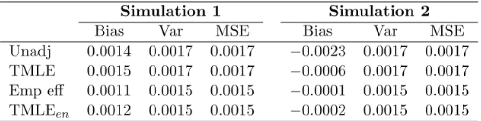
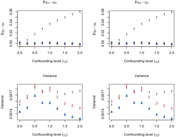
Figure 1 summarizes results for simulation 3a with bounds on gn(1 | W) set to (10−9,1−10−9) and (0.1, 0.9). The bias of the unadjusted estimator (1) in-creases with γ2, while the TMLE (2), Emp Eff (3), and TMLEen (4) estimators remain unbiased. When confounding is strong, the unadjusted estimator has the highest variance, followed by TMLE, while as predicted by theory, the variance of the TMLEen estimator closely matches that of the empirical efficiency estimator, designed to minimize variance. Because the treatment assignment mechanism does not lead to a violation of the positivity assumption (0.14< g0(1|W)<0.77), results are the same regardless of the choice of truncation level for gn(1|W). Estimator performance under increasing practical violations of the positivity assumption is il-lustrated in Figure 2, which shows results at three truncation levels of gn(1 |W), (10−9,1−10−9), (0.025, 0.975), and (0.1, 0.9). Increasing truncation introduces a small amount of bias into TMLE, the empirical efficiency maximization estimator,

1 1 1 1 1 1 1 1 1 0.0 0.5 1.0 1.5 2.0 0.00 0.02 0.04 0.06 Eψn−ψ0 Confounding level (γ2) E ψn − ψ0 2 2 2 2 2 2 2 2 2 3 ₃ 3 3 3 3 3 3 ₃ 4 _{4 4} 4 4 4 4 4 4 ₁ 1 1 1 1 1 1 1 1 0.0 0.5 1.0 1.5 2.0 0.00 0.02 0.04 0.06 Eψn−ψ0 Confounding level (γ2) E ψn − ψ0 2 2 2 2 2 2 2 2 2 3 ₃ 3 3 3 3 3 3 ₃ 4 _{4 4} 4 4 4 4 4 4 1 1 1 1 1 ₁ 1 1 1 0.0 0.5 1.0 1.5 2.0 0.0014 0.0017 Variance Confounding level (γ2) Variance 2 2 2 2 2 2 2 2 2 3 3 3 3 3 3 3 ₃ 3 4 4 4 4 4 4 4 4 ₄ 1 1 1 1 1 ₁ 1 1 1 0.0 0.5 1.0 1.5 2.0 0.0014 0.0017 Variance Confounding level (γ2) Variance 2 2 2 2 2 2 2 2 2 3 3 3 3 3 3 3 3 ₃ 4 4 4 4 4 4 4 4 ₄

Figure 1: Simulation 3a: Estimator bias and variance at each value of γ2, two truncation levels for gn(1 | W), (10−9,1−10−9) (left), and (0.1, 0.9) (right). 1: Unadjusted, 2: TMLE, 3: Emp Eff, 4: TMLEen.

and TMLEen, but this amount is dwarfed by the bias of the unadjusted estima-tor. We observe that the variance of all but the unadjusted estimator increases with increased confounding, and is slightly ameliorated by increased truncation of

gn(1|W). At extreme violations of the positivity assumption (Table 3) the variance of TMLEen(4) is slightly larger than that of the empirical efficiency maximization estimator (3), but overall these two estimators are very close to one another.

6

Discussion

The TMLE represents a template for construction of a loss-based substitution es-timator of a target parameter defined on a semiparametric model, defined by a choice of loss function for a relevant part of the data generating distribution, a parametric submodel, and a strategy for iteratively minimizing the empirical risk

1 1 1 1 1 1 0.0 0.2 0.4 0.6 0.8 1.0 0.00 0.02 0.04 0.06 0.08 0.10 Confounding level (γ1) E ψn − ψ0 2 2 2 2 2 2 3 3 3 3 3 3 4 4 4 4 4 4 1 1 1 1 1 1 0.0 0.2 0.4 0.6 0.8 1.0 0.00 0.02 0.04 0.06 0.08 0.10 Eψn−ψ0 Confounding level (γ1) E ψn − ψ0 2 2 2 2 2 2 3 3 3 3 3 3 4 4 4 4 4 4 1 1 1 1 1 1 0.0 0.2 0.4 0.6 0.8 1.0 0.00 0.02 0.04 0.06 0.08 0.10 Confounding level (γ1) E ψn − ψ0 2 2 2 2 2 2 3 3 3 3 3 3 4 4 4 4 4 4 1 ₁ 1 1 1 1 0.0 0.2 0.4 0.6 0.8 1.0 0.0016 0.0018 0.0020 0.0022 Confounding level (γ1) Variance 2 2 2 2 2 2 3 3 3 3 3 3 4 4 4 4 4 4 1 ₁ 1 1 1 1 0.0 0.2 0.4 0.6 0.8 1.0 0.0016 0.0018 0.0020 0.0022 Variance Confounding level (γ1) Variance 2 2 2 2 2 2 3 3 3 3 3 3 4 4 4 4 4 4 1 ₁ 1 1 1 1 0.0 0.2 0.4 0.6 0.8 1.0 0.0016 0.0018 0.0020 0.0022 Confounding level (γ1) Variance 2 2 2 2 2 2 3 3 3 3 3 3 4 4 4 4 4 4

Figure 2: Simulation 3b: Estimator bias and variance at each value ofγ1. Columns correspond to truncation level for gn(1 | W), (10−9,1−10−9) (left), (0.025, 0.05) (middle), and (0.1, 0.9)(right). 1: Unadjusted, 2: TMLE, 3: Emp Eff, 4: TMLEen.

Table 3: True conditional treatment assignment probabilities as a function ofγ1. γ1 Range of g0(A|W) γ1 Range of g0(A|W)

0 0.305 0.551 0.6 0.035 0.926

0.2 0.212 0.676 0.8 0.013 0.969

0.4 0.090 0.837 1 0.005 0.987

over the parametric submodel. The choice of submodel and loss function defines the score equations the TMLE will solve. In this manner it can be arranged that the TMLE solves not only the efficient score equation, but also an estimating equation corresponding with the influence curve of a competing estimator. By solving this estimating equation the TMLE is at least as efficient as the competing estimator in the case this competing estimator is asymptotically linear andg0_n is consistent.

We demonstrated this type of TMLE for the simple point treatment data struc-ture (W, A, Y) and the additive effect parameter. Our presentation is straightfor-wardly generalized to general CAR-censored data models, and target parameters, since we only relied on a general representation of the efficient influence curve as an augmented IPCW-function as presented in Robins and Rotnitzky (1992); van der Laan and Robins (2003). Suppose now that the target parameter is multivariate. One needs to define the collection of real valued parameters, and one needs to de-fine a competing estimator for each of these real valued parameters. For example, one might define one single real valued parameter as a function of the multivariate parameter, or one might define each component of the target parameter as a real valued parameter. Each of the real valued parameters implies now an influence curve of the corresponding competing estimator. Each of these influence curves implies a clever covariate for the treatment mechanism playing the role of H(Qe_n, g_nk) in the above TMLE algorithm. The resulting TMLE will not only be a double robust locally efficient substitution estimator of the target parameter, but it will also esti-mate each of the real valued parameters in a more efficient way than the competing estimators, in the case thatg0 is estimated consistently.

References

W. Cao, A.A. Tsiatis, and M. Davidian. Improving efficiency and robustness of the doubly robust estimator for a population mean with incomplete data.Biometrika, 96,3:723–734, 2009.

S. Gruber and M.J. van der Laan. An application of collaborative targeted maximum likelihood estimation in causal inference and genomics. The International Journal of Biostatistics, 2010a.

S. Gruber and M.J. van der Laan. A targeted maximum likelihood estimator of a causal effect on a bounded continuous outcome. The International Journal of Biostatistics, 6:1(26), 2010b.

J. Pearl. Causality: Models, Reasoning, and Inference. Cambridge University Press, Cambridge, 2nd edition, 2000.

J.M. Robins and A. Rotnitzky. Recovery of information and adjustment for depen-dent censoring using surrogate markers. In AIDS Epidemiology, Methodological issues. Bikh¨auser, 1992.

A. Rotnitzky, Q. Lei, M. Sued, and J. Robins. Enhanced double-robust locally-efficient estimation in regression models for longitudinal studies. Presentation ENAR 2011 Spring Meeting, article submitted, March 2011.

D.B. Rubin and M.J. van der Laan. Empirical efficiency maximization: Improved lo-cally efficient covariate adjustment in randomized experiments and survival anal-ysis. The International Journal of Biostatistics, Vol. 4, Iss. 1, Article 5, 2008. Z. Tan. Bounded, efficient, and doubly robust estimation with inverse weighting.

Biometrika, 94:1–22, 2008.

R Development Core Team. R: A Language and Environment for Statistical Com-puting. R Foundation for Statistical Computing, Vienna, Austria, 2010.

M. J. van der Laan. The construction and analysis of adaptive group sequential de-signs. Technical Report 232, www.bepress.com/ucbbiostat/paper232, University of California, Berkeley, 2008.

M.J. van der Laan and S. Dudoit. Unified cross-validation methodology for selection among estimators and a general cross-validated adaptive epsilon-net estimator: Finite sample oracle inequalities and examples. Technical report, Division of Biostatistics, University of California, Berkeley, November 2003.

M.J. van der Laan and J.M. Robins. Unified methods for censored longitudinal data and causality. Springer, New York, 2003.

M.J. van der Laan and S. Rose.Targeted Learning: Prediction and Causal Inference for Observational and Experimental Data. Springer, New York, 2011.

M.J. van der Laan and D. Rubin. Targeted maximum likelihood learning. The International Journal of Biostatistics, 2(1), 2006.

M.J. van der Laan, E. Polley, and A. Hubbard. Super learner.Statistical Applications in Genetics and Molecular Biology, 6(25), 2007. ISSN 1.

W. Zheng and M. J. van der Laan. Asymptotic theory for

cross-validated targeted maximum likelihood estimation. Technical Report 273, www.bepress.com/ucbbiostat/paper273, University of California, Berkeley, 2010.

Appendix: R Implementation

The R function below calculates the enhanced TMLE for binary outcomes. Required arguments are Y (binary outcome vector), A (binary treatment indicator vector), and initial estimates ¯Q0_n(A, W), g0_n(A | W), and f_ne(W). Q¯0_n(A, W) is an n×3 matrix containing values for ¯Q0_n(A, W),Q¯0_n(0, W), and ¯Q0_n(1, W) on the logit scale. Predicted values for gn(A|W) are bounded away from 0 and 1.

bound <- function(x, bounds){ x[x<min(bounds)] <- min(bounds) x[x>max(bounds)] <- max(bounds) return(x) } tmle_en <- function(Y, A, g1W, Q, f, gbds = c(10^-9, 1-10^-9)){ g1w <- bound(g1W, gbds)

eps1 <- eps2 <- Inf epsilon <- .00001 maxIter <- 30 iterations <- 0

while((any(abs(c(eps1, eps2)) > epsilon)) & iterations <= maxIter){ iterations <- iterations + 1

h <- cbind(A/g1W - (1-A)/(1-g1W), 1/g1W, -1/(1-g1W))

m <- glm(Y ~ -1 + offset(Q[,"QAW"]) + h[,1], family=binomial) eps1 <- coef(m)

Q <- Q + eps1*h

h2 <- plogis(Q[,"Q1W"])/g1W + plogis(Q[,"Q0W"])/(1-g1W) h3 <- f/(g1W * (1-g1W))

g <- glm(A ~ -1 + offset(qlogis(g1W)) + h2 + h3, family=binomial)

g1W <- bound(predict(g, type = "response"), gbds) eps2 <- coef(g)

}

Q <- plogis(Q)

psi.en <- mean(Q[,"Q1W"] - Q[,"Q0W"])

psi.IPTW <- mean((A/g1W - (1-A)/(1-g1W)) * Y)

psi.AIPTWQstargstar <- mean((A/g1W - (1-A)/(1-g1W)) * Y

- (Q[,"Q1W"]/g1W - Q[,"Q0W"]/(1-g1W))*(A-g1W))

psi.AIPTWQegstar <- mean((A/g1W - (1-A)/(1-g1W)) * Y

- f/(g1W * (1-g1W)) * (A-g1W))

return(c(psi.en, psi.IPTW, psi.AIPTWQstargstar, psi.AIPTWQegstar)) }