Basic and Applied Research
(IJSBAR)
ISSN 2307-4531 (Print & Online)
http://gssrr.org/index.php?journal=JournalOfBasicAndApplied
---
Effect of Akaike Information Criterion on Model Selection
in Analyzing Auto-crash Variables
Osuji G. A.
a*, Okoro C. N.
b, Obubu M.
c, Obiora-Ilouno H. O.
da,b,c ,d
Department of Statistics, Nnamdi Azikiwe University, P.M.B. 5025, Awka, Anambra State, Nigeria.
b
Email: [email protected]
Abstract
Count data has become widely available in many disciplines. The mostly used distribution for modeling count data is the Poisson distribution (Horim and Levy; 1981) which assume equidispersion (Variance is equal to the mean). Since observed count data often exhibit over or under dispersion, the Poisson model becomes less ideal for modeling. To deal with a wide range of dispersion levels, Generalized Poisson regression, Poisson regression, and lately Conway-Maxwell-Poisson (COM-Poisson) regression can be used as alternative regression models. We compared the Generalized Poisson regression, Poisson Regression Model and Conway- Maxwell- Poisson. Data on road traffic crashes from the Anambra State Command of the Federal Road Safety Commission (FRSC), Nigeria were analyzed using these three methods, the results from the three methods are compared using the Akaike Information Criterion (AIC) with Poisson showing an AIC value of 2325.8 and GPR having an AIC value of 896.0278 and COM-Poisson showing an AIC value of 951.01. The GPR was considered a better model when analyzing road traffic crashes in Anambra State, Nigeria.
Keywords: Over-dispersion; Road Traffic; Crashes; Discrete; Akaike Information Criterion; equidispersion.
--- * Corresponding author.
1. Introduction
Count data arise in many fields which includes; biology, healthcare, psychology, marketing and many more. When response variable is a count and the researcher is interested in how this count changes as the explanatory variable increases. Classical Poisson regression is the most well-known methods for modeling count data, but its underlying assumption of equidispersion limits its use in many real-world applications with over-or under dispersed data. This excess variation may result to incorrect inference about parameter estimates, standard errors, tests and confidence intervals. Over-dispersion mostly arises for various reasons including mechanisms that generate excessive zero counts or censoring. As a result over-dispersed count data are common in many areas which in turn, have led to the development of statistical methodology for modeling over-dispersed data [1]. For over-dispersed data, the Negative Binomial model is a popular choice [2]. Other over-dispersion models include Poisson mixtures [3] and Conway-Maxwell-Poisson. A flexible alternative that captures both over- and under-dispersion is the Conway-Maxwell-Poisson (COM-Poisson) distribution. The COM-Poisson is a two-parameter generalization of the Poisson distribution which also includes the Bernoulli and Geometric distributions as special cases [4]. The COM-Poisson distribution has been used in so many count data application and has been extended methodologically in various directions [1]. Therefore in this work, because of the problem of model selection and the appropriate method to apply in the analysis of auto-crash data bearing in mind their underlying assumptions, we wish to find the model that is most adequate.
2. Methodology
In this section we shall review the models that most widely used in the analysis of count data which include: the Poisson models, Conway- Maxwell- Poisson models, Generalized Poisson Regression model and the Akaike Information Criterion
2. 1 Poisson Models
This is a special case of Generalized Linear Models (GLM) framework. The simplest distribution used for modeling count data is the Poisson distribution with probability density function
P(𝑌𝑌𝑖𝑖 = 𝑦𝑦𝑖𝑖) = 𝜆𝜆𝑖𝑖𝑦𝑦𝑖𝑖exp(−𝜆𝜆𝑖𝑖)
𝑦𝑦𝑖𝑖! 𝑦𝑦1 = 0,1,2, … (1)
The canonical link is (𝜇𝜇)= log(𝜇𝜇) resulting in a log-linear relationship between mean and linear predictor. The
variance in the Poisson model is identical to the mean, thus the dispersion is fixed at 𝜙𝜙=1 and the variance
function is V(𝜇𝜇)=𝜇𝜇 [5]. The mean Poisson regression can be assumed to follow a log link, (𝑌𝑌i)=𝜇𝜇i=𝑒𝑒𝑥𝑥𝑝𝑝(𝑥𝑥i′𝛽𝛽),
where 𝑥𝑥idenotes the vector of explanatory variables and β the vector of regression parameters. The maximum
likelihood estimates can be obtained by maximizing the log likelihood.
2.2 Conway-Maxwell-Poisson (COM-Poisson) Models
enough to describe a wide range of count data distributions, since its revival, it has been further developed in several directions and applied in multiple fields.
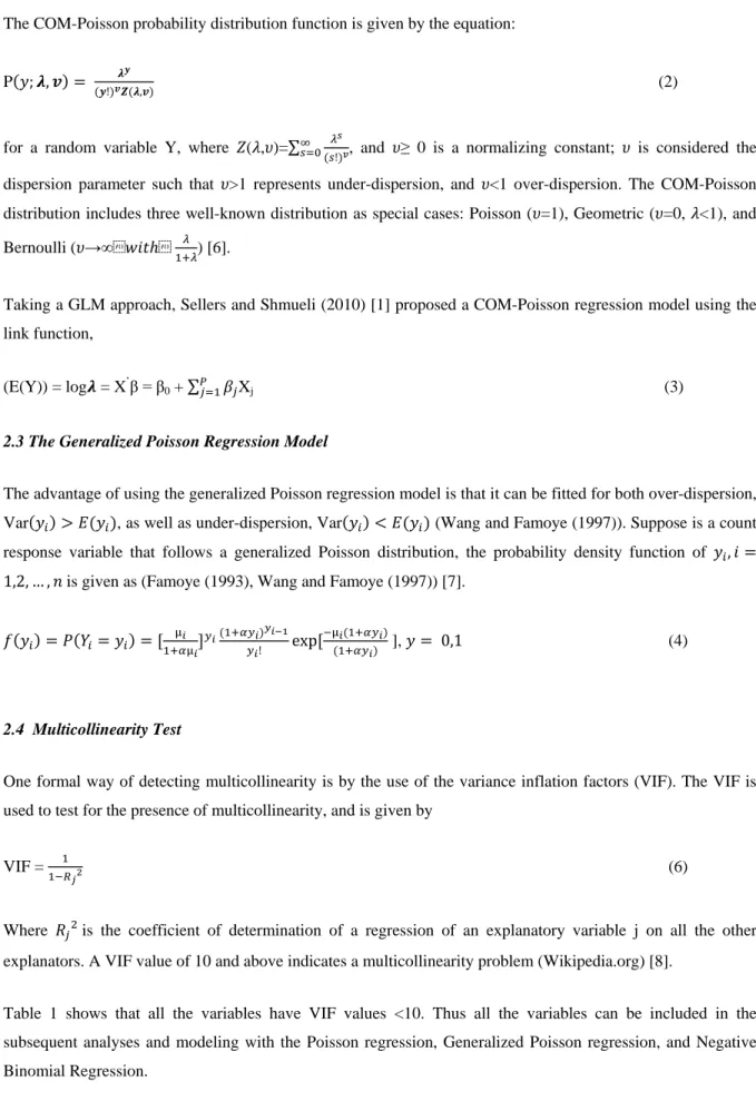
The COM-Poisson probability distribution function is given by the equation:
P(𝑦𝑦;𝝀𝝀,𝒗𝒗) = (𝒚𝒚!)𝒗𝒗𝝀𝝀𝒁𝒁(𝝀𝝀,𝒗𝒗)𝒚𝒚 (2)
for a random variable Y, where 𝑍𝑍(𝜆𝜆,𝜐𝜐)=∑𝑠𝑠=0∞ (𝑠𝑠!)𝜆𝜆𝑠𝑠𝑣𝑣, and 𝜐𝜐≥ 0 is a normalizing constant; 𝜐𝜐 is considered the
dispersion parameter such that 𝜐𝜐>1 represents under-dispersion, and 𝜐𝜐<1 over-dispersion. The COM-Poisson
distribution includes three well-known distribution as special cases: Poisson (𝜐𝜐=1), Geometric (𝜐𝜐=0, 𝜆𝜆<1), and Bernoulli (𝜐𝜐→∞𝑤𝑤𝑖𝑖𝑡𝑡ℎ1+𝜆𝜆𝜆𝜆 ) [6].
Taking a GLM approach, Sellers and Shmueli (2010) [1] proposed a COM-Poisson regression model using the link function,
(E(Y)) = log𝝀𝝀 = X’β = β0 + ∑𝑃𝑃𝑗𝑗=1𝛽𝛽𝑗𝑗Xj (3)
2.3 The Generalized Poisson Regression Model
The advantage of using the generalized Poisson regression model is that it can be fitted for both over-dispersion, Var(𝑦𝑦𝑖𝑖) >𝐸𝐸(𝑦𝑦𝑖𝑖), as well as under-dispersion, Var(𝑦𝑦𝑖𝑖) <𝐸𝐸(𝑦𝑦𝑖𝑖) (Wang and Famoye (1997)). Suppose is a count
response variable that follows a generalized Poisson distribution, the probability density function of 𝑦𝑦𝑖𝑖,𝑖𝑖=
1,2, … ,𝑛𝑛is given as (Famoye (1993), Wang and Famoye (1997)) [7].
𝑓𝑓(𝑦𝑦𝑖𝑖) =𝑃𝑃(𝑌𝑌𝑖𝑖=𝑦𝑦𝑖𝑖) = [1+𝛼𝛼µµ𝑖𝑖 𝑖𝑖] 𝑦𝑦𝑖𝑖(1+𝛼𝛼𝑦𝑦𝑖𝑖)𝑦𝑦𝑖𝑖−1 𝑦𝑦𝑖𝑖! exp [ −µ𝑖𝑖(1+𝛼𝛼𝑦𝑦𝑖𝑖) (1+𝛼𝛼𝑦𝑦𝑖𝑖) ], 𝑦𝑦= 0,1 (4) 2.4 Multicollinearity Test
One formal way of detecting multicollinearity is by the use of the variance inflation factors (VIF). The VIF is used to test for the presence of multicollinearity, and is given by
VIF = 1
1−𝑅𝑅𝑗𝑗2 (6)
Where 𝑅𝑅𝑗𝑗2is the coefficient of determination of a regression of an explanatory variable j on all the other
explanators. A VIF value of 10 and above indicates a multicollinearity problem (Wikipedia.org) [8].
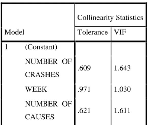
Table 1 shows that all the variables have VIF values <10. Thus all the variables can be included in the subsequent analyses and modeling with the Poisson regression, Generalized Poisson regression, and Negative Binomial Regression.
Table 1: Multicollinearity Test Model Collinearity Statistics Tolerance VIF 1 (Constant) NUMBER OF CRASHES .609 1.643 WEEK .971 1.030 NUMBER OF CAUSES .621 1.611
2.5 Akaike Information Criterion (AIC)
When several models are available, one can compare the models performance based on several likelihood measures which have been proposed in statistical literatures. One of the most popularly used measures is AIC. The AIC penalized a model with larger number of parameters, and is defined as
𝐴𝐴𝐼𝐼𝐶𝐶=−2𝑙𝑙𝑛𝑛𝐿𝐿+2𝑝𝑝 (7)
Where 𝑙𝑙𝑛𝑛𝐿𝐿 denotes the fitted log likelihood and 𝑝𝑝 the number of parameters. A relatively small value of AIC is
favorable for the fitted model [6].
3. Analysis and Results
The data were analyzed using R Software and the results obtained are given below. Before performing the analysis on the three methods used, testing the data for multicollinearity was conducted. The test results are shown in table II below:
5. Conclusion
Poisson regression model, GPR, and Conway-Maxwell- Poisson regression model were compared to determine a better model used in modeling auto-crashes in Anambra State, Nigeria. The criterion for selection of the best model used is AIC. Best model is the model that has the smallest AIC value.
6. Recommendation
Based on AIC values in Table 1, the smallest AIC value is a Generalized Poisson Regression model. Thus, the best model for analyzing traffic crash data or over and under-dispersed data is the Generalized Poisson Regression model.
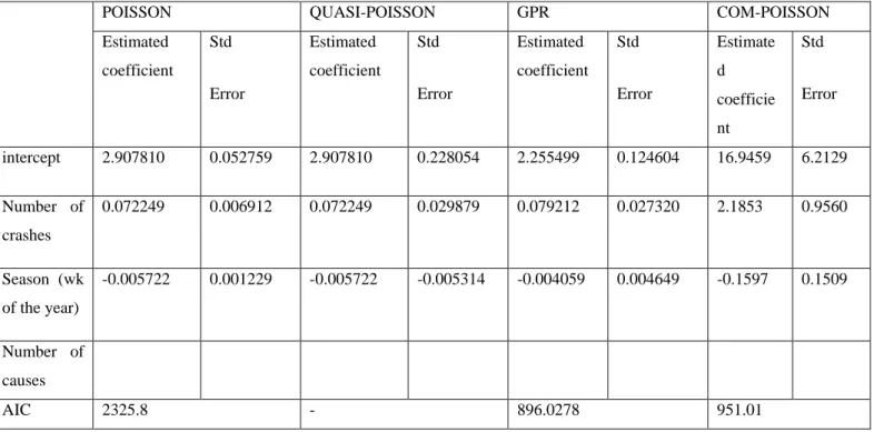
Table 2: Parameter estimates, standard error and AIC value for models
POISSON QUASI-POISSON GPR COM-POISSON
Estimated coefficient Std Error Estimated coefficient Std Error Estimated coefficient Std Error Estimate d coefficie nt Std Error intercept 2.907810 0.052759 2.907810 0.228054 2.255499 0.124604 16.9459 6.2129 Number of crashes 0.072249 0.006912 0.072249 0.029879 0.079212 0.027320 2.1853 0.9560 Season (wk of the year) -0.005722 0.001229 -0.005722 -0.005314 -0.004059 0.004649 -0.1597 0.1509 Number of causes AIC 2325.8 - 896.0278 951.01 References
[1] K.F. Sellers, G. Shmueli G, Data Dispersion: Now you see it...Now you don't, Communication in
Statistics: Theory and Methods. 42, Issue 17, 3134-47 (2013).
[2] J.M. Hilbe,"Negative Binomial Regression". 2nd edition. Cambridge University Press, London (2011). [3] G.J. McLachlan, On the EM Algorithm for Overdispersed Count Data, Statistical Methods in Medical
Reseach.6, 76-98 (1997).
[4] G. Shmueli, T.P. Minka, J.B. Kadane, S. Borle, P. Boatwright, A Useful Distribution for Fitting Discrete Data: Revival of the Conway–Maxwell–Poisson Distribution, Journal of The Royal Statistical Society. Series C (Applied Statistics). 54, Issue 1, 127-142 (2005).
[5] A. Zeileis, C. Kleiber, S. Jackman, Regression Models for Count Data in R, Journal of Statistical Software. 27, Issue 8, 1-25 (2008).
[6] Bozdogan, H. (2000). “Akaike's Information Criterion and Recent Developments in Information Complexity”. Mathematical Psychology, 44 , 62-91.
[7] Famoye (1993), Wang and Famoye (1997),” Restricted Generalized Poisson Regression Model”. Communication in statistics -Theory and Methods. 01/1993; 22(5): 1335-1354. DOI: 10.1080/03610929308831089
[8] Wikipedia.org
[3] Cameron, A.C and Trivedi, P. K (1998), “Regression analysis of count data.” Cambridge University press Cambridge, UK.
[4] Consul P. C. and Famoye F. (1992), “Generalized Poisson regression model”, communications in statistics (theory and methodology) vol. 2, no.1, 89-109.
[5] S.D. Guikema, J.P. Coffelt, A Flexible Count Data Regression Model for Risk Analysis, Risk Analysis.
28, Issue 1, 213-223 (2008).
[6] D. Lord, S.R. Geedipally, S.D. Guikema, Extension of the Application of Conway-Maxwell-Poisson
Models: Analyzing Traffic Crash Data Exhibiting Under-Dispersion, Risk Analysis. 30, Issue 8,
1268-1276 (2010).
[7] Famoye F, John T. W. and Karan P. S. (2004), “On the generalized Poisson regression model with an application to accident data”. Journal of data science 2 (2004), 287-295.
Appendix >y= c(47,23,19,11,9,23,30,71,65,7,55,8,46,76,3,67,10,18,10,30,0,6,61,47,67,35,81,67,46,12,32,11,41,22,44,16,0,12, 29,25,31,15,4,5,84,45,61,27,0,35,20,72,44,35,10,33,85,10,42,0,14,11,95,82,45,61,47,70,32,7,18,42,19,20,9,11,9 ,23,30,71,53,12,0,7,31,0,33,8,7,50,33,5,2,32,3,6,4,4,1,0,85,44,3,16) > x1 = c(5,4,10,6,3,6,1,1,7,7,7,6,2,1,3,3,1,8,3,2,0,10,11,5,1,4,6,4,7,2,5,4,4,2,4,2,0,3,2,5,2,6,1,1,5,6,8,7,0,3,10,6,4,2,2,2, 6,2,1,0,3,2,11,10,11,5,10,7,8,8,7,4,5,4,10,6,6,1,1,3,9,4,0,2,4,0,7,2,2,4,2,2,1,7,1,1,1,2,1,0,8,4,1,3) > x2 = c(1,2,3,4,5,6,7,8,9,10,11,12,13,14,15,16,17,18,19,20,21,22,23,24,25,26,27,28,29,30,31,32,33,34,35,36,37,38,39, 40,41,42,43,44,45,46,47,48,49,50,51,52,1,2,3,4,5,6,7,8,9,10,11,12,13,14,15,16,17,18,19,20,21,22,23,24,25,26,2 7,28,29,30,31,32,33,34,35,36,37,38,39,40,41,42,43,44,45,46,47,48,49,50,51,52) > x3 = c(5,4,3,2,3,3,1,1,7,7,7,6,2,1,3,3,1,8,3,2,0,3,3,5,1,4,6,4,7,2,5,4,4,2,4,2,0,3,2,5,2,6,1,1,5,6,8,7,0,3,3,6,4,2,2,2,6,2,1, 0,3,2,3,4,5,1,4,2,3,2,3,4,5,4,3,2,2,1,1,3,3,4,0,2,4,0,3,2,2,4,2,2,1,2,1,1,1,2,1,0,2,1,1,3)
> local({pkg <- select.list(sort(.packages(all.available = TRUE)),graphics=TRUE)
Loading required package: stats4 Loading required package: splines
> model = vglm(y~x1+x2+x3, family = genpoisson)
Warning message:
In log(theta + x * lambda) : NaNs produced
> summary(model)
Call:
vglm(formula = y ~ x1 + x2 + x3, family = genpoisson) Pearson residuals:
Min 1Q Median 3Q Max
rhobit(lambda) -0.6557 -0.5331 -0.2506 0.4613 2.7072
loge(theta) -4.4189 -0.3801 0.3893 0.8479 0.9771
Coefficients:
Estimate Std. Error z value Pr(>|z|)
(Intercept):1 2.255499 0.124604 18.101 < 2e-16 *** (Intercept):2 0.996075 0.200239 4.974 6.54e-07 *** x1 0.079212 0.027320 2.899 0.003739 ** x2 -0.004059 0.004649 -0.873 0.382701 x3 0.137679 0.040374 3.410 0.000649 *** --- Signif. codes: 0 ‘***’ 0.001 ‘**’ 0.01 ‘*’ 0.05 ‘.’ 0.1 ‘ ’ 1
Number of linear predictors: 2
Names of linear predictors: rhobit(lambda), loge(theta)
Dispersion Parameter for genpoisson family: 1
Log-likelihood: -443.0139 on 203 degrees of freedom
Number of iterations: 13
> AIC(model)
[1] 896.0278
> model = glm(y~x+x2+x3, family = poisson) Error in eval(expr, envir, enclos) : object 'x' not found
> model = glm(y~x1+x2+x3, family = poisson)
> summary(model)
Call:
glm(formula = y ~ x1 + x2 + x3, family = poisson)
Deviance Residuals:
Min 1Q Median 3Q Max
-8.100 -3.884 -1.411 2.021 9.565
Coefficients:
Estimate Std. Error z value Pr(>|z|)
(Intercept) 2.907810 0.052759 55.115 < 2e-16 ***
x1 0.072249 0.006912 10.452 < 2e-16 ***
x2 -0.005722 0.001229 -4.654 3.25e-06 ***
---
Signif. codes: 0 ‘***’ 0.001 ‘**’ 0.01 ‘*’ 0.05 ‘.’ 0.1 ‘ ’ 1
(Dispersion parameter for poisson family taken to be 1)
Null deviance: 2276.6 on 103 degrees of freedom
Residual deviance: 1840.5 on 100 degrees of freedom
AIC: 2325.8
Number of Fisher Scoring iterations: 5
> local({pkg <- select.list(sort(.packages(all.available = TRUE)),graphics=TRUE) + if(nchar(pkg)) library(pkg, character.only=TRUE)})
> model.nb = glm(y~x1+x2+x3)
> summary(model.nb)
Call:
glm(formula = y ~ x1 + x2 + x3)
Deviance Residuals:
Min 1Q Median 3Q Max
-42.656 -14.817 -7.673 11.592 56.389
Coefficients:
Estimate Std. Error t value Pr(>|t|)
(Intercept) 16.9459 6.2129 2.728 0.00754 **
x1 2.1853 0.9560 2.286 0.02438 *
x2 -0.1597 0.1509 -1.059 0.29233
---
Signif. codes: 0 ‘***’ 0.001 ‘**’ 0.01 ‘*’ 0.05 ‘.’ 0.1 ‘ ’ 1
(Dispersion parameter for gaussian family taken to be 517.7724)
Null deviance: 64857 on 103 degrees of freedom
Residual deviance: 51777 on 100 degrees of freedom
AIC: 951.01
Number of Fisher Scoring iterations: 2
> model.compis = glm.compois(y~x1+x2+x3) Error: could not find function "glm.compois"
> model.compois = glm.compois(y~x1+x2+x3)
Error: could not find function "glm.compois"
> model.compois =glm(y~x1+x2+x3)
> summary(model.compois)
Call:
glm(formula = y ~ x1 + x2 + x3)
Deviance Residuals:
Min 1Q Median 3Q Max -42.656 -14.817 -7.673 11.592 56.389
Coefficients:
Estimate Std. Error t value Pr(>|t|)
(Intercept) 16.9459 6.2129 2.728 0.00754 **
x2 -0.1597 0.1509 -1.059 0.29233 x3 2.7158 1.4705 1.847 0.06771 .
---
Signif. codes: 0 ‘***’ 0.001 ‘**’ 0.01 ‘*’ 0.05 ‘.’ 0.1 ‘ ’ 1
(Dispersion parameter for gaussian family taken to be 517.7724)
Null deviance: 64857 on 103 degrees of freedom
Residual deviance: 51777 on 100 degrees of freedom
AIC: 951.01
Number of Fisher Scoring iterations: 2
> local({pkg <- select.list(sort(.packages(all.available = TRUE)),graphics=TRUE)
+ if(nchar(pkg)) library(pkg, character.only=TRUE)})
> local({pkg <- select.list(sort(.packages(all.available = TRUE)),graphics=TRUE)
+ if(nchar(pkg)) library(pkg, character.only=TRUE)})
> model.compois =glm(y~x1+x2+x3)
> summary(model.compois)
Call:
glm(formula = y ~ x1 + x2 + x3) Deviance Residuals:
Min 1Q Median 3Q Max
-42.656 -14.817 -7.673 11.592 56.389
Coefficients:
(Intercept) 16.9459 6.2129 2.728 0.00754 ** x1 2.1853 0.9560 2.286 0.02438 * x2 -0.1597 0.1509 -1.059 0.29233 x3 2.7158 1.4705 1.847 0.06771 . --- Signif. codes: 0 ‘***’ 0.001 ‘**’ 0.01 ‘*’ 0.05 ‘.’ 0.1 ‘ ’ 1
(Dispersion parameter for gaussian family taken to be 517.7724)
Null deviance: 64857 on 103 degrees of freedom Residual deviance: 51777 on 100 degrees of freedom
AIC: 951.01