A State-Space Model for the Dynamic Random
Subgraph Model
Rawya Zreik, Pierre Latouche, Charles Bouveyron
To cite this version:
Rawya Zreik, Pierre Latouche, Charles Bouveyron. A State-Space Model for the Dynamic
Random Subgraph Model. European Symposium on Artificial Neural Networks, Computational
Intelligence and Machine Learning (ESANN), Apr 2015, Bruges, Belgium. pp.231-236.
<
hal-01199634
>
HAL Id: hal-01199634
https://hal.archives-ouvertes.fr/hal-01199634
Submitted on 15 Sep 2015
HAL
is a multi-disciplinary open access
archive for the deposit and dissemination of
sci-entific research documents, whether they are
pub-lished or not.
The documents may come from
teaching and research institutions in France or
abroad, or from public or private research centers.
L’archive ouverte pluridisciplinaire
HAL
, est
destin´
ee au d´
epˆ
ot et `
a la diffusion de documents
scientifiques de niveau recherche, publi´
es ou non,
´
emanant des ´
etablissements d’enseignement et de
recherche fran¸
cais ou ´
etrangers, des laboratoires
publics ou priv´
es.
A State-Space Model for the Dynamic Random
Subgraph Model
Rawya ZREIK1,2, Pierre LATOUCHE1 and Charles BOUVEYRON2 1- Laboratoire SAMM, EA 4543, Universit´e Paris 1 Panth´eon-Sorbonne
2- Laboratoire MAP5, UMR CNRS 8145, Universit´e Paris Descartes
Abstract. In recent years, many random graph models have been
pro-posed to extract information from networks. The principle is to look for groups of vertices with homogenous connection profiles. Most of these models are suitable for static networks and can handle different types of edges. This work is motivated by the need of analyzing an evolving net-work describing email communications between employees of the Enron compagny where social positions play an important role. Therefore, in this paper, we consider the random subgraph model (RSM) which was proposed recently to model networks through latent clusters built within known partitions. Using a state space model to characterize the cluster proportions, RSM is then extended in order to deal with dynamic net-works. We call the latter the dynamic random subgraph model (dRSM).
1
Introduction
Network analysis has become an independent discipline which is no longer limited to sociology and is now applied in many areas such as biology, geography or history. The most recent statistical methods for the modeling and processing of the data are generally based on the stochastic block model (SBM) [1]. The SBM model assumes that each vertex belongs to a latent group, and that the probability of connection between a pair of vertices depends exclusively on their group. Among the recent extensions of the SBM model, we consider the random subgraph model (RSM) proposed by Jerniteet al. [2]. The RSM model aims at modeling categorical edges using prior knowledge of a partition of the network into subgraphs. The subgraphs are assumed to be made of latent clusters which have to be inferred from the data in practice. The vertices are then connected with a probability depending only on the subgraphs whereas the edge type is assumed to be sampled conditionaly on the latent groups. In this work, we propose to extend the RSM model in order to deal with dynamic networks. The proposed model is called the dynamic random subgraph model (dRSM). A
state-space model (SSM) is considered to characterize the temporal evolution of the cluster mixing proportions. The inference of this model is made through a variational EM (VEM) algorithm. The methodology is eventually applied to the famous Enron dataset describing the evolution of electronic communications between employees for two years (2001-2002). Figure 1 presents the evolution of the e-mail communication network for the four months before the financial collapse of the company in December 2001.
August 2001 September 2001 October 2001
November 2001
CEO, presidents Vice−presidents, directors Managers, managing directors Traders Employees Unknowns
Fig. 1: Electronic communication network between 148 Enron employees during the 4 months (August-December 2001) before the bankruptcy of the company.
2
The dynamic random subgraph model
We consider a set ofTnetworks{G(t)}T
t=1, whereG(t)is a directed graph observed at timet and for which a partitionP(t) into S subgraphs is also known. Each
G(t) is represented by itsN ×N adjacency matrixX(t) where N denotes the number of nodes (assumed constant over time). No self loops are considered. The edge Xij(t), describing the relationship between nodes i and j, is assumed
to take its values in{0, . . . C} such thatXij(t)=c means that nodesiand j are
linked by a relationship of typec at timet andXij(t)= 0 indicates the absence
of relationship. Our goal is to cluster at each timettheN nodes intoK latent groups with homogeneous connection profiles,i.e. find an estimate at each time t of the binary matrix Z which is such thatZik(t) = 1, if at time t, the node i belongs to the classk, and 0 otherwise.
2.1 The model at each time t
The network is assumed to be generated at each timetas follows. Each vertexiis first associated to a latent classkwith a probability depending on the subgraph which it belongs to. We assume, that for a given number K of latent groups, the variableZi(t) is drawn from a multinomial distribution of parameterα
(t) si: Zi(t)∼ M(1, α (t) si), where α(st)= (α( t) s1, . . . , α (t)
sK) is the vector of prior probabilities of theK latent
groups in the subgraphsat timetand is such thatPK
k=1α
(t)
sk = 1,∀s∈1, . . . , S.
On the other hand, we assume that the type of link between nodes i and j is sampled from a multinomial distribution depending on the latent vectors Zi(t)
andZj(t)as follows:
Xi,j(t)|Zik(t)Zjl(t)= 1∼ M(1,Πkl),
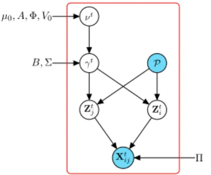
Xt ij Π Zt i Zt j P γt B,Σ νt µ0, A,Φ, V0
Fig. 2: The graphical model for dRSM.
2.2 Modeling of the evolution of the random subgraphs
We introduce now a hidden state, in the form of astate-space model [3, chapter 13] to capture the dynamic behavior of the proportions of the latent classes within the subgraphs over time. In order to apply this model, we introduce a new latent variableγs(t)which is assumed to be distributed according to a normal
distribution with meanBν(t)and covariance matrix Σ, where:
ν(t)=Aν(t−1)+ω γs(t)=Bν(t)+v ν(1)=µ0+u.
The noise terms ω, uand v are supposed to be Gaussian: ω ∼ N(0,Φ), v ∼ N(0,Σ), u∼ N(0, V0). Aand B are two transition matrices of size (K−1)×
(K−1). We finally assume a logistic link between the latent group proportions α(st)and the hidden variableγ(
t)
s in the form ofαs=f(γs) where,
α(skt)= exp(γsk(t)−C(γ(t) s )), ∀k= 1, . . . , K, (1) and C(γs(t)) = P K `=1exp(γ (t)
s`). Thus, the state-space model of γ
(t) allows us to characterize the temporal process of the latent group proportions. Due to the bijectivity constrain of this logistic transformation, α(st) only has K −1
degree of freedom. Thus, we only need to draw the first K−1 components of γ(st) in which the last component is arbitrarily set to zero, to generateα(
t)
s .
Finally, our model has three latent variables (ν, γ, Z) and is parameterized by θ= (µ0, A, B,Φ, V0,Σ,Π) where the vectorµ0has (K−1) components, whereas (A, B,Φ, V0,Σ) are (K−1)×(K−1) matrices. This model is called the dy-namic random subgraph model (dRSM). Figure 2 presents the graphical model for dRSM.
2.3 Inference with VEM algorithm for the dRSM model
We aim at maximizing the log-likelihood logp(X|θ) associated with the model. To achieve this maximization, a common approach consists in using an EM
algo-rithm. However, such an algorithm connot be derived here sincep(Z|X, θ) is in-tractable. Therefore, we propose to use a variational EM-type algorithm (VEM), which locally optimizes the model parameters with respect to a lower bound of the log-likelihood. Traditionally, the VEM algorithm focuses on optimizing a lower bound of the form L(q, θ) = P
z R γ R νq(Z, γ, ν) log p(X, Z, γ, ν|θ) q(Z, γ, ν) dγ dν. Unfortunately, because logp(Z|α=f(γ)) involves here a non linear transforma-tion, additional approximations are required. Making use of a Taylor expansion for the term logC(γs(t)), we derive the following inequality:
logp(Z|α)) ≥ T X t=1 K X k=1 N X i=1 YisZ( t) ik γ(skt)− ξ−1(t) s K X l=1 exp(γsl(t))−1 + log(ξ(t) s ) (2) = logh(Z, γ, ξ), (3) where ξt
s ∈ R∗+ is a new variational parameter. Replacing logp(Z|f(γ)) by
logh(Z, γ, ξ) in L(q, θ), a new lower bound ˜L(q, θ) for logp(X|θ) is obtained. We finally assume thatq(Z, γ, ν) can be factorized, that is:
q(Z, γ, ν) =q(Z)q(γ)q(ν) = T Y t=1 N Y i=1 q(Zi(t) T Y t=1 q(γ(t) T Y t=1 q(ν(t),
andq(γ) is a product of normal distributions of parameters ˆγsk(t) ,ˆσ
(t) sk: q(γ) = T Y t=1 S Y s=1 K−1 Y k=1 N(γsk(t); ˆγsk(t),σˆ(skt)2).
The VEM update step (E-step) for the distributionq(Zi(t)) is given by:
q(Zi(t))∼ M(Z
(t)
i ; 1, τ
(t)
i ) ∀i, t.
However, for the distribution of q(ν), it was not possible to identify a usual probability distribution, but we recognized the distribution associated with a
state-space model. Thus, the corresponding parameters can be estimated using the standard Kalman filter and Rauch-Tung-Striebel (RTS) smoother equations.
q(ν)∝p(ν(1)|µ0, V0)h T Y t=2 p(ν(t)|ν(t−1), A,Φ)ih T Y t=1 p( PS s=1ˆγ (t) s S |ν (t),Σ S, B) i ,
whereν(t)is a latent variable andx(t)=
PS
s=1γˆ (t)
s
S seen as an observed variable such thatx(t)=Cν(t)+ ˜v and ˜v∼ N(0,Σ
S).
In the M-step of the VEM algorithm updating formulas for the parameters Π and ξcan be obtained by maximizing the lower bound ˜L(q, θ). Updates for ˆ
γs(tik) and ˆσ
(t)2
sl have however to be found by numerically maximizing ˜L(q, θ) using
t periods t1 from 01/01/2000 to 01/12/2000 t2 from 01/01/2001 to 01/03/2001 t3 from 01/04/2001 to 01/06/2001 t4 from 01/07/2001 to 01/09/2001 t5 from 01/10/2001 to 01/03/2002 Table 1: The time periods for the study.
3
Application to the Enron network
In this section, we apply our methodology to the Enron data set, which de-scribes the exchange of emails among 148 individuals who have worked for the Enron company at each timet. We are interested here in five time periods noted t1, t2, . . . , t5 (Table 1). A partition of the employees into three subgraphs de-pending on their status in the company (Managers, Employees, Others) is also available. The network is a directed and binary network without self loops,i.e.
C= 1 andXt
ij = 1 ifiandjexchanged at least one email during the periodt, 0
otherwise, witht∈ {1, . . . ,5}andS= 3. We used the variational EM algorithm introduced in the previous section in order to look for K = 4 latent groups in the data.
3.1 Results
Since the network is binary, the dRSM model used here is a special case of the model we proposed with C = 1. By construction, the matrix Π verifies Πkl0+ Πkl1= 1,∀(k, l) therefore, only the Πkl1terms describing the connections probabilities are given in Table 2. Table 2 shows that the three clusters (1, 2 and 4) correspond to the communities where the probability of connection between two nodes of the same community is stronger than between different communities nodes. Thus, these clusters are mainly distinguished that they have different intra-cluster probabilities of connection, where the cluster 1 has the highest density (0.478), followed by the clusters 2 and 4 . Finally, the cluster 3 is built from low probabilities of connection (0.001). It gathers in fact at all individuals participating in non structured exchange in the network.
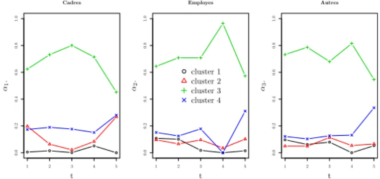
Applying our dRSM model on the Enron network allows the characterization of the subgraphs evolution with latent clusters according to the time. Figure 3 presents all estimated proportions of three subgraphs. We observe a drop in the proportion of cluster 3, in all subgraphs betweent4 andt5,i.e. just before and after the opening of the investigation by the US federal agency. This specific network structure is here a reaction to the crisis of October 2001. The employees exchange emails on the subject and contact people preferentially. At this period, the proportion of cluster 4 (lower intra-cluster density), such as the one of cluster 3, increase. It is worth noticing that the structuring of the network starts earlier (att3) among managers than among employees. The subgraphs 2 and 3 have a
cluster 1 cluster 2 cluster 3 cluster 4 cluster 1 0.478 0.037 0.005 0.023 cluster 2 0.020 0.181 0.006 0.012 cluster 3 0.001 0.002 0.001 0.003 cluster 4 0.012 0.012 0.024 0.119
Table 2: Terms Πkl1 of the matrix Π estimated using the VEM algorithm
1 2 3 4 5 0.0 0.2 0.4 0.6 0.8 1.0 Cadres t α1 . 1 2 3 4 5 0.0 0.2 0.4 0.6 0.8 1.0 Employes t α2 . cluster 1cluster 2 cluster 3 cluster 4 1 2 3 4 5 0.0 0.2 0.4 0.6 0.8 1.0 Autres t α3 .
Fig. 3: Proportions of theK= 4 clusters, at each time. Subgraph 1 (Managers), left figure; subgraph 2 (employees), middle figure; subraph 3 (other), right figure.
mild reaction to others, but it disappears att4. This observation suggests that managers were aware of the arrival of the crisis before other employees. Finally, the cluster 1 with high intra-cluster density allows to see that the managers are the only individuals in the network for which we observe a diminution in the proportion of the cluster 1 at the time (t4, t5) unlike the subgraphs 2 and 3. Finally, through these observations and by taking into consideration the high position of managers where the exchange of emails is very preferable, allows to be separated the managers from the rest of the network.
References
[1] Y.J. Wang and G.Y. Wong. Stochastic blockmodels for directed graphs. Journal of the
American Statistical Association, 82:8–19, 1987.
[2] Y. Jernite, P. Latouche, C. Bouveyron, P. Rivera, L. Jegou, and S. Lamass´e. The random
subgraph model for the abalysis of an acclesiasrical network in merovingian gaul. Annals
of Applied Statistics, 2013.