2011/22
!
VAR forecasting using Bayesian variable selection
Dimitris Korobilis
Center for Operations Research
and Econometrics
Voie du Roman Pays, 34
B-1348 Louvain-la-Neuve
Belgium
http://www.uclouvain.be/core
CORE DISCUSSION PAPER 2011/22
VAR forecasting using Bayesian variable selection Dimitris KOROBILIS1
May 2011
Abstract
This paper develops methods for automatic selection of variables in Bayesian vector autoregressions (VARs) using the Gibbs sampler. In particular, I provide computationally efficient algorithms for stochastic variable selection in generic linear and nonlinear models, as well as models of large dimensions. The performance of the proposed variable selection method is assessed in forecasting three major macroeconomic time series of the UK economy. Databased restrictions of VAR coefficients can help improve upon their unrestricted counterparts in forecasting, and in many cases they compare favorably to shrinkage estimators.
Keywords: forecasting, variable selection, time-varying parameters. JEL Classification: C11, C32, C52, C53, E37
1 Université catholique de Louvain, CORE, B-1348 Louvain-la-Neuve, Belgium.
E-mail: [email protected].
This paper presents research results of the Belgian Program on Interuniversity Poles of Attraction initiated by the Belgian State, Prime Minister's Office, Science Policy Programming. The scientific responsibility is assumed by the author.
1
Introduction
Since the pioneering work of Sims (1980), a large part of empirical macroeconomic modeling is based on vector autoregressions (VARs). Despite their popularity, the flexibility of VAR models entails the danger of over-parameterization, which can lead to poor forecasts. This pitfall of VAR modelling was recognized early, and in response shrinkage methods have been proposed; see for example the so-called Minnesota prior (Doan, Litterman and Sims, 1984). Nowadays the applied econome-tricians’ toolbox includes numerous ecient modelling tools to prevent the prolifer-ation of parameters and eliminate parameter and model uncertainty: variable selec-tion priors (George, Sun and Ni, 2008), steady-state priors (Villani, 2009), Bayesian model averaging (Garratt, Koop, Mise and Vahey, 2009) and factor models (Stock and Watson, 2006), to name but a few.
This paper develops a stochastic search algorithm for variable selection in lin-ear and nonlinlin-ear vector autoregressions (VARs) using Markov Chain Monte Carlo (MCMC) methods. The term “stochastic search” simply means that if the model space is too large to assess in a deterministic manner (that is, enumerate and es-timate all possible models, and decide on the best one using some goodness-of-fit measure), the algorithm will visit only the most probable models in a stochastic man-ner. In this paper, the general model form that I am studying is the reduced-form VAR model, which can be written using the following linear regression specification yt =c+B1yt1+B2yt2+...+Bpytp+t (1)
whereyt is anm1 vector oft= 1, ..., T time series observations on the dependent
variables and the errorstare assumed to beN(0,), whereis anmmcovariance
matrix. The idea behind Bayesian variable selection is to introduce indicators ij
such that
Bij = 0 ifij = 0 (2)
Bij = 0 ifij = 1
where Bij is an element of the mk coecient matrix B =
i= 1, .., m, j= 1, ..., k andk =p+ 1.
There are various benefits of using this approach over some of the shrinkage methods mentioned previously, such as the Minnesota prior or factor models. First, variable selection is automatic, meaning that along with estimates of the parameters we get associated probabilities of inclusion of each parameter in the “best” model. In that respect, the variables ij indicate which elements of B should be included or excluded from the final optimal model. Selection of the optimal model is im-plemented among all possible 2n, n = mk, VAR model combinations, without the
need to estimate each and every one of these models. Second, this form of Bayesian variable selection is independent of the prior assumptions about the coecientsB. That is, if the researcher has defined any desirable prior for the parameters of the unrestricted model (1), adopting the variable selection restriction (2) needs no other modification than adding one extra block in the posterior sampler that draws from the conditional posterior of the ij’s. An indirect implication of this approach is that, unlike other proposed stochastic search variable selection algorithms for VAR models (George et al. 2008; Korobilis, 2008), variable selection of this form may be adopted in VAR models which are nonlinear in the mean coecients B.
In fact, in this paper I show that variable selection is very easy to adopt in the non-linear and richly parameterized, time-varying parameters vector autoregression (TVP-VAR). These models are currently very popular for measuring monetary pol-icy and have been used extensively in academic research (Canova and Gambetti, 2009; Cogley and Sargent, 2002; Cogley, Morozov and Sargent, 2005; Koop, Leon-Gonzalez and Strachan, 2009; and Primiceri, 2005). Common feature of these papers is that they all fix the number of autoregressive lags to 2 for parsimony. This simpli-fication is so popular because marginal likelihoods are dicult to obtain, especially in the presence of stochastic volatility where one has to rely on computationally expensive particle filtering methods (Koop and Korobilis, 2009a). Even if we as-sume that marginal likelihoods are readily available, these would allow only pairwise comparisons and hence all 2n TVP-VAR models need to be estimated. Therefore, automatic variable selection is a convenient and fast way to overcome the com-putational and practical problems associated with (comcom-putationally) demanding nonlinear VAR models as well as simple linear models.
selection on several VAR formulations with various prior specifications. In particular I begin with the simple linear VAR model with ridge regression, Minnesota, and adaptive shrinkage priors. Following this, variable selection for nonlinear models is introduced, where in addition to the TVP-VAR I consider a multivariate extension of the Koop and Potter (2007) structural breaks autoregressive model which allows to forecast breaks out-of-sample. Finally, given the recent interest in forecasting with large models (Ba´nbura, Giannone and Reichlin, 2010) as an alternative to dimension reduction using principal components (Stock and Watson, 2006), a modification of the stochastic restriction search useful for VARs of medium and large dimensions is established.
Although the methods described in this paper can be used for structural analysis (by providing data-based restrictions on the coecients which could enhance iden-tifying monetary policy for instance), the aim is to show how more parsimonious models can be selected to have a positive impact on macroeconomic forecasting.
The next section describes the mechanics behind variable selection in a general VAR setting. In Section 3, variable selection is established for specific cases of linear VAR models of small and larger dimensions, and nonlinear models. The paper concludes by evaluating the out-of-sample forecasting performance of VAR models using variable selection, for three key UK macroeconomic variables observed over the period 1971:Q1 - 2008:Q4.
2
Variable selection in vector autoregressions
To allow for dierent equations in the VAR to have dierent explanatory variables, rewrite equation (1) as a system of seemingly unrelated regressions (SUR)
yt=zt+t (3)
where zt = Im xt = Im (1, yt1, ..., ytp) is a matrix of dimensions m n,
=vec(B)isn1, and
t N(0,). When no parameter restrictions are present
in equation (3), this model will be referred to as the unrestricted model. Bayesian variable selection is incorporated by defining and embedding in model (3) indicator
variables = (1, ...,n), such that j = 0 ifj = 0, and j = 0 if j = 1. These indicators are treated as random variables by assigning a prior on them, and allowing the data likelihood to determine their posterior values. We can explicitly insert these indicator variables multiplicatively in the model1 using the following
form
yt =zt+t (4)
where = . Here is an nn diagonal matrix with elements jj = j on its
main diagonal, for j = 1, ..., n. It is easy to verify that when j = jj = 0 then
j is restricted and is equal to jjj = 0, while for j = jj = 1 it holds that
j = jjj = j, so that all possible 2n VAR specifications can be explored and
variable selection in this case is equivalent to model selection.
2.1
A generic VAR case
The restricted VAR specification (4) may serve as a generic formulation for the rest of the models. All we have to do is make sure that we can write the linear/nonlinear VAR models in SUR form. For instance, in the next section I show that when using nonlinear models we can arrive in a SUR form similar to equation (4), but in this case it will hold that = g(). Here g() is any class of nonlinear functions of the VAR parameters , with a prior densityF(·), that is
p(g())F(a, G0) (5)
In this paper I focus on specifications of interest to macroeconomists who usually assume that g() is a piecewise linear function (as it is the case with the class of structural breaks, Markov Switching and threshold autoregressive specifications, among others) but generalizations to other nonlinear or nonparametric functions is almost as straightforward.
Derivations are simplified if the indicators j are a priori independent of each other for j = 1, ..., n, i.e. p() =jn=1pj=nj=1pj|\j, where \j indexes
all the elements of a vector but the jth. Additionally, we can remove the eect of the covariance matrix by integrating this parameter using an a scale invariant
improper Jerey’s prior. Hence we have
j|\j Bernoulli(0j) (6)
||(m+1)/2 (7) where0j is the prior probability of the Bernoulli density, implying prior belief that
coecient j is restricted.
The following pseudo-algorithm demonstrates that the algorithm for the re-stricted model (4) actually adds only one block (which samples the restriction in-dicators ) over the standard algorithm of the unrestricted VAR model (3). In the rest of the paper I define y = (y1, ..., yT) and z= (z1, ..., zT).
Bayesian Variable Selection Pseudo-Algorithm
1. Sampleg()from the conditional posterior (assuming it exists)2 of the form
g()|, y, z,L(y, z;g()|,)F(a, G0)
where L(y, z;g()|,)is the conditional likelihood (i.e. conditional on,
being known). Here z
t is the restricted data matrix withzt=zt
2. Sample eachj conditional on\j,g(), and the data from
j|\j, g(),, y, zBernoulli(0j) (8)
preferably in random order j, j= 1, ..., n, where j = l0jl+0jl1j, with
l0j = p y|j,,\j,j = 1 0j (9) l1j = p y|j,,\j,j = 0 (10j) (10)
3. Sample as in the unrestricted VAR in (3), where now the mean equation
2For all the popular nonlinear models I consider, the posterior conditionals exist, so that a
parameters are =g().
1|,, y, zW ishart,S1 (11)
where =T and S=Tt=1(yt+hzt)(yt+hzt)
.
In this type of model selection, what we care about is which of the parameters
are equal to zero, so that identifiability of g()and plays no role. In a Bayesian setting identifiability is still possible, since if the likelihood does not provide infor-mation about a parameter, its prior does. When for a specific j= 1, .., nwe sample agj= 0 thenj is identified by drawing from its prior: notice that in this case in equations (9) - (10) it holds thatpy|j,\j,j = 1
=py|j,\j,j = 0
,so that the posterior probability of the Bernoulli density,j, will be equal to the prior
probability 0j. Similarly, when j = 0 then g
j is identified from its prior: the j-th column of zt = zt will be zero, i.e. the likelihood provides no information
aboutgj, and sampling from the posterior ofgj collapses to getting a draw from its prior. Nevertheless, in both of the above cases the result of interest is that thej-th parameter should be restricted sincej = 0.
Posterior computation is based on Gibbs sampler with complete blocking. If the support of is finite (see also the discussion of priors on in the next section), then we can use the argument of Tierney (1991) to show that the Markov Chain is geometrically ergodic and that a Central Limit Theorem on this Markov Chain is available. Thus, convergence of the Gibbs sampler is expected to be quite rapid, and selection of the correct restrictions quite accurate. A simulation study in the working paper version of this article confirms that this is the case for both linear and nonlinear VAR models in small samples.
3
VAR formulations and priors
This section describes in detail some popular VAR specifications and various prior distributions on them that are considered in the empirical application of this paper. The main idea is to compare all linear and nonlinear VAR formulations using some popular priors routinely used in business and academia, with and without variable
selection. First, I show how each of these popular VAR models admit a SUR form. Then the model with variable selection is the one where the j’s are sampled from (8), and the corresponding unrestricted model is the one where we simply impose
j = 1 j without sampling from the posterior (as it will be clear in Section 4, this model is also equivalent to imposing the tight prior 0j = 1 j on the restricted
model). Some of the priors described here already provide some shrinkage (i.e. they provide data-based rules to restrict irrelevant VAR coecients). This fact implies that we can examine how variable selection competes with traditional shrinkage (for instance the Minnesota prior), but also if combining variable selection and shrinkage priors in the same VAR model could help improve forecasting even further.
In order to do such a comparison, the intercepts are left unrestricted (j = 1 if j is an intercept) and flat priors are placed on them in all instances. Similarly the covariance matrix is integrated out with the improper scale invariant (Jerey’s) prior in equation (7). Finally, the hyperparameters 0j found in equation (6) are
set to 0j = 0.8 implying that 80% of the predictors should be included in the
final model. This assumption is reasonable for small trivariate VARs, since the “noninformative” choice 0j = 0.5 implies that probably too many (i.e. 50%) VAR
coecients should be restricted. In subsection 3.4 I introduce variable selection specifically for large VARs. There I relax this assumption and propose setting the values of0j in the spirit of the Minnesota prior (i.e. penalize heavily more distant
lags using the variable selection algorithm) which can assist in solving the curse of dimensionality problem in these models. Full Bayes and Empirical Bayes priors can also be used on0j and the reader can seek more information in Chipman, George
and McCulloch (2001).
3.1
Linear VAR
The traditional VAR process with variable selection is fully described by equation (4), where (and hence = ) enters the model linearly. Typical prior distribu-tions for linear VAR models are based on the Normal density, i.e.
In this paper I examine three types of eliciting prior hyperparameters based on the Normal distribution, all of which provide some form of shrinkage in the VAR coecients (but no exact zero restrictions like variable selection does).
Ridge regression prior This is probably the most widely used prior in
autore-gressive models. The assumption is that b = 0n1 and V = In. The posterior
mean/mode of the Bayes estimator is equal to the penalized least squares estimator which writes
=zz+1In
1 zy
which is equivalent to unrestricted LS for . The reader should also note that for the case (in practical situations this translates to = 100 and above) variable selection cannot be performed. An intuitive explanation for this eect is that marginal likelihoods for model selection cannot be calculated with uninformative priors. Kuo and Mallick (1997) give a more detailed explanation about this issue and propose to use values of [0.25,25]. Consequently, in the absence of prior information about the model coecients, one can use a locally uninformative prior by setting = 100 (diuse prior) on the intercepts and = 9 for autoregressive coecients. In near-covariance stationary VAR processes the autoregressive coecients are expected to be roughly less than one in absolute value, so a higher value of for these parameters is basically redundant.
Minnesota (Litterman) prior The Minnesota prior is very popular and is as
old as the VAR literature in economics. This prior is due to the works of Bob Litterman and colleagues at Minnesota University and the Minneapolis Fed; see for instance Litterman (1986) and Doan, Litterman and Sims (1984). This Empirical Bayes formulation assumes the prior mean vectorb is set equal to1 for parameters on the first own lag of each variable (random walk prior) and zero otherwise, and V is a diagonal matrix with diagonal element the variance on lagr of variable j in equation iof the form
Vrij = 100s2i if intercept 1/r2 if i=j s2i r2s2 l if i=j (12)
for r= 1, ..., p, i= 1, ..., m,and j = 1, ..., k with k =p+ 1. Here s2
i is the residual
variance from the unrestricted p-lag univariate autoregression for variable i. The degree of shrinkage depends on a single hyperparameter 3, where again if
we end up with unrestricted estimates similar to LS. Litterman (1986) originally introduced a hyperparameter for own lags as well, i.e. he usedVrij =/r2 ifi=jin equation (12). For small and medium VAR models it is the choice ofthat matters. I set = 1 which provides a “realistic” prior variance for own lag coecients. In covariance-stationary VARs we do not expect these coecients to be much larger than 1 especially for higher order lags, so1/r2should (and does) work fine. Selection of in contrast is dependent on the specific dataset and application considered. Selection of the shrinkage factorof the Minnesota prior is discussed in subsection 4.1.
Hierarchical Bayes Shrinkage prior Shrinkage priors based on Empirical Bayes
methods, like the Minnesota prior, suer from the fact that they are subjective con-structs and might not appeal to the objective researcher. The formal Bayesian way to shrinkage in regressions is to use hierarchical priors on the regression coecients so that the shrinkage parameter is chosen objectively by the data. In Korobilis (2011) I show that using hierarchical Normal-Gamma priors, we can recover many popular shrinkage estimators for sparse signals, like the least absolute shrinkage and selection operator (LASSO) of Tibshirani (1996) and its variants (Fused LASSO, Group LASSO, Elastic Net). Here I use a special case of adaptive shrinkage Normal-Gamma priors which is the hierarchical Normal-Jerey’s prior of Hobert and Casela (1993) of the form Nn(0, V), Vjj=j, j = 1, ..., n j 100 1/j if j is an intercept coecient otherwise (13)
3Litterman (1986) originally introduced a hyperparameter for own lags as well, i.e. he used
Vrij = /r2 if i = j in equation (12). For small and medium VAR models it is the choice of
that matters. I set = 1which provides a “realistic” variance for own lag coecients (we do not expect these coecients to be much larger than 1).
In simple words, by placing a scale invariant Jereys’ distribution on j, its
pos-terior value is determined solely by the data (hence is not a prior choice for the researcher). This is the simplest form of adaptive shrinkage, and can easily be used in VAR models. In Korobilis (2011) I show that LASSO-based Bayesian shrink-age (specifically the hierarchical version of the Elastic Net algorithm of Zou and Hastie, 2005) perform even better in forecasting than simple Normal-Jereys priors. However as explained in Park and Casela (2008) for LASSO-type priors we need to condition j on the model error variance, something not straightforward to do in a VAR model, unless we make simplifying assumptions like setting to be diagonal.
3.2
Time-varying parameters VAR
Modern macroeconomic applications increasingly involve the use of VARs with mean regression coecients and covariance matrices which drift every month/quarter. Nonetheless, forecasting with time-varying parameters VARs is not a new topic in economics. During the “Minnesota revolution” ecient approximation methods of forecasting with TVP-VARs were developed, with most notable contributions the ones by Doan, Litterman and Sims (1984) and Sims (1989); for a large-scale ap-plication in an 11-variable VAR see also Canova (1993). Using modern posterior simulator methods (Markov Chain Monte Carlo), TVP-VARs have been used re-cently very extensively for structural analysis (Primiceri, 2005; Cogley and Sargent, 2002) and forecasting (D’Agostino et al., 2009; Cogley et al., 2005), while Groen, Paap and Ravazzolo (2009) and Koop and Korobilis (2009b) are focusing on uni-variate predictions with the use of a large set of exogenous variables.
As mentioned in the Introduction, marginal likelihood calculations in this model are hard to implement. When specifically stochastic volatility is present, computa-tionally expensive particle filtering methods are needed only to obtain a measure of fit for a single model. Estimation using Bayesian variable selection is not aected by specific modelling assumptions (like the inclusion or not of stochastic volatility) and can accommodate all possible model combinations eciently in a single run of the Gibbs sampler.
(Homoskedas-tic TVP-VAR) takes the form
yt =ct+B1,tyt1+...+Bp,tytp+t (14)
where as before t N(0,)with anmmcovariance matrix. This model can
easily be written in the variable selection SUR form (4), by definingtto be then1 vectorc t, vec B 1,t , ..., vecB p,t of parameters andzt =Im(1, yt1, ..., ytp) is
an mn matrix. In that case we have
yt = ztt+t (15)
t = t1+t (16)
where t = t and is the nn matrix defined in (4). Equation (16) defines a
random walk evolution of the nonlinear VAR coecients4, for which it holds that
t N(0, Q)with Q annn covariance matrix.
Note that variable selection in this case implies that a VAR coecient either enters or exits the “true” model in all time periods t = 1, ..., T. In contrast, to-day there are methods in univariate regressions which allow dierent coecients to be selected at dierent points in time. Most notably, Chan, Koop, Leon-Gonzalez and Strachan (2010) use such a flexible specification, however estimation relies on computationally intensive MCMC procedures which only allow them to consider a handful of variables. The ecient approximations we describe in Koop and Koro-bilis (2009b) allow dynamic model averaging (DMA) and selection (DMS) with up to around 20 predictors (i.e. to average or select among 220 models at each period t). Nonetheless, the smallest typical VAR used in macroeconomics has three quar-terly variables and four lags and an intercept (39 mean coecients), which makes application of DMA computationally intensive.
While the priors for (,) are the same as in the previous cases (Jerey’s-Bernoulli), it can be shown that conjugate priors for the remaining parameters of
4An autoregressive model of order one could be defined, but early empirical experience with
the TVP-VAR model (Cogley and Sargent, 2002) are of the form
0 Nn(b, V)
Q1 W ishart, R1
with 0 being practically the initial condition of t. Note that a prior on each
t, t = 1, ..., T, need not be specified since this is implicitly defined recursively as
t Nn
t1, Q. An important thing to underline is that the model allows the VAR coecientst to evolve as random walks forT periods, so that shrinkage/tight priors must be used especially forQ(a detailed explanation why is given in Primiceri, 2005, Section 4.4). Cogley and Sargent (2005) and Primiceri (2005) use the OLS estimates of a simple VAR estimated on a training sample to inform their prior hyperparameters, and set their shrinkage coecient (what was denoted as in the linear VAR priors) at a very small value. This approach is standard in Bayesian analysis, especially when marginal likelihoods are not readily available, but it results in discarding valuable information in the training sample.
In contrast the standard Minnesota prior can be used to inform the initial con-dition 0 of the TVP-VAR coecients, combined with a tight prior on Q. Subse-quently, we can set b and V as in equation (12), while setting = 2 (n+ 1) and R = kRIn5, where n is the number of coecients in t and kR is a scaling factor
which we have to choose. Following Cogley and Sargent’s (2002) “business as usual” prior, i.e. the belief that the TVP-VAR coecients should vary smoothly and not change abruptly each time period, I setkR = 0.0001. This is the standard value used
by Primiceri after implementing a sensitivity analysis, see Primiceri (2005, Section 4.4.1). Consequently, as in the linear VAR models, we only need to worry about the value of the shrinkage coecient , a choice which is discussed in the empirical section.
5To replicate Primiceri’s (2005) training sample prior, we can use R= k
RV where as before
V is the Minnesota prior covariance matrix. However this assumption does not alter any of the forecasting results for the UK dataset used in the empirical section.
3.3
Structural breaks VAR
In theory and in practice, a VAR with structural breaks lies between the linear VARs (zero breaks) and the TVP-VAR (breaks in every period, i.e. T breaks) and should have been presented earlier. However one of all the possible formulations of structural breaks in the VAR coecients, which is due to Koop and Potter (2007), is to write the model as a special case of the TVP-(V)AR presented above. Subse-quently, following equations (15) and (16) we can write the structural breaks VAR using the form
yt = ztst +t (17)
st = st
1+st. (18)
Herest =st,t N(0, Q), andst [1, ..., K + 1]is a first order Markov process with block-diagonal transition matrix of the form
P = p11 p12 0 · · · 0 0 p22 p23 . .. ... .. . . .. ... ... 0 0 pKK pK,K+1 0 · · · 0 0 pK+1
which makes the structural breaks model a restricted form of a Markov switching VAR, since we can only move from one regime to the next, and never return to a previous regime. In this case we have a breaks between time periodtandt+1ist=
st+1. Uncertainty about the number of regimes is easily incorporated in a Bayesian context by setting a maximum number of breaks, say Kmax, and allowing the data to determine the “true” number of estimated breaks K, where 1 K Kmax. In Bauwens, Koop, Korobilis and Rombouts (2011) we give exact implementation details on forecasting with a univariate version of this model, which I follow closely in this multivariate extension. Estimation details are provided in the Appendix.
covariance matrix, Q1 W ishart(, R1), are based on Sims’s version of the Minnesota prior explained in the previous subsection. The additional parameters on this model are the transition probabilities pij = Pr [st =i|st1 =j], for which I use the typical Beta prior for the diagonal elements pii Beta(1,2),i= 1, ..., K. For1=2 = 1this density becomes uniform and noninformative. The parameters st are estimated as in Chib (1996).
3.4
Extension to large VARs and comparison with other
models
The fact that automatic Bayesian variable selection is stochastic and simulation is needed (Gibbs sampler) implies that it’s use is in general prohibitive in VARs with hundreds of dependent variables as in Ba´nbura, Giannone and Reichlin (2010). Moreover, the disadvantage of variable selection is that in order to allow dierent variables to enter dierent equations, the SUR form of the VAR is needed which relies on inverting large matrices (since the RHS data matrix iszt =Imxt instead of just
xt in the reduced-form VAR). Even so, this subsection discusses some modifications
to variable selection that would make its usage in medium-sized VARs possible. Consider the linear VAR6 model (1) written compactly as
yt =Bxt+t where xt = (1, yt1, ..., ytp)and B = c, B 1, ..., Bp is mk. Instead of restricting individually each of the n = mk elements of B, when m is “large” we might want to consider restricting only the k columns of B. This simplification implies that a specific RHS variable yi,tj,i [1, m], j [1, p] either enters simultaneously in all
m VAR equations or none. While this results in a loss of modelling flexibility, the implication is that when we model, say,m= 15variables in a VAR withp = 4lags we only need to average across 260 models as opposed to the2900 models available
6Obviously treating large nonlinear VARs is not dierent. However this is not discussed, since
large time-varying parameters and structural breaks VARs are computationally intensive. In Ko-robilis (2011b) I derive ecient computational methods to forecast with VARs of very large di-mensions (whetherT ormare in the order of thousands) in seconds of computer time.
otherwise. More importantly, we do not need the computationally expensive SUR form to estimate the VAR model, since we can now write the large VAR + model selection model as
yt =xt+t
where = B with the kk diagonal matrix with the restriction indices on its diagonal.
It would be of benefit to relax the assumption that the prior on the indicesj is Bernoulli with “uninformative” hyperparameter 0j = 0.5. It is feasible to impose
many restrictions a priori by setting 0 <0j 0.57. For instance 0j = 0.1 means
that our expectation is that 90% of the coecients should be restricted. However, we need not impose these restrictions linearly on all parameters. Following the Minnesota tradition we can use a prior which restricts a priori coecients on more distant lags
0j =
0.5, for own lags 1/(r+ 1), otherwise where r= 1, .., p.
The idea to restrict the VAR regression coecients can also be extended to finding restrictions in the covariance matrix of a VAR. In fact, Smith and Kohn (2002) and Wong, Carter and Kohn. (2003), take the Cholesky decomposition1= AAof anmmcovariance matrix, and impose restrictions on the matrixAusing
indicator variables, say . In this decomposition is a diagonal matrix and A is a lower triangular matrix with 1’s on the diagonal. Hence model selection proceeds by setting
i = 0 ifi = 0
i = 0 ifi = 0
7The alternative
0j >0.5 imposes the prior belief that not many restrictions are expected in
the VAR coecients. If the researcher is uncertain about these beliefs, a Beta prior can always be placed on0jwhich makes this hyperparameter an unknown random variable to be updated from
whereiis each of them(m1)/2non-zero and non-one elements ofA. Therefore,
similarly to the case of variable selection in the mean equation coecients, their approach can be easily generalized to a covariance matrix which is stochastic as for example in the popular Heteroskedastic TVP-VARs of Primiceri (2005), Canova and Gambetti (2009) and Cogley and Sargent (2002). Considering covariance matrix selection and assuming dierent functional forms for the covariance matrix (say time-varying, or structural breaks) will aect forecasts to some extent and would not allow to evaluate the performance of variable selection in the mean VAR equation, which is of prime interest since it has much larger number of coecients. For that reason, it is better to integrate out the (constant) covariance matrix, as well as the intercepts, using uninformative priors as is the standard practice in the Bayesian Statistics literature when evaluating model selection or shrinkage priors (see among others Park and Casella, 2008; Villani, 2009; and Liang, Paulo, Molina, Clyde and Berger, 2008).
There are several other approaches to automatic Bayesian model selection and shrinkage for univariate regression models which can be generalized to VAR models. The formal “full-Bayes” procedure as it is called, is based on hierarchical Normal priors of the form
| Nn(0n1,V)
F (a, b, c) (19)
where V is a prior covariance matrix and F(·) denotes a density function with parameters a, b, c. In this case, if the prior distribution of , F(a, b, c), is the Bernoulli() then takes only the values 0 and 1 and we have model selection identical to the one described above (if = 1 the prior is (| = 1) Nn(0, V),
if = 0 the prior is (|= 0) Nn(0n1,0nn), i.e. a Dirac point mass at
zero). This is the case of the stochastic search variable selection (SSVS) prior used in George, Sun and Ni (2008), Korobilis (2008) and Jochmann, Koop and Strachan (2010). As discussed in subsection 3.1 if we assume V = In and we assign a prior
for of the form Gamma(1,2)then we can have shrinkage of dependent on whether the 0 or 0. Additionally, the shrinkage priors have the de-sirable property that they become variable/model selection priors in models with more predictors than observations; see Korobilis (2011).
From a practitioner’s point of view, it must be noted that the SSVS prior as well as adaptive shrinkage priors of this hierarchical form are computationally much faster than variable selection considered in this paper. The main issue with Hi-erarchical Gaussian priors is that they cannot be used in nonlinear VARs like the TVP-VAR, which are of special interest to academics and practitioners in Central Banks. A hierachical prior like (19) can be potentially applied to the initial con-dition of the TVP-VAR, which would take the form 0| Nn(0,V). We can
immediately observe that for the subsequent time periods, the prior on the time-varying coecients becomest Nn
t1, Qso that dependence on the shrinkage properties ofis lost, and the prior mean becomest1which in general will be esti-mated from the likelihood to be other than zero. To the best of my knowledge there are no formal Bayesian model selection or shrinkage estimators for these nonlinear VARs and the focus of this paper is to fill this gap using the methods described so far.
4
Macroeconomic forecasting with VARs
The variable selection techniques described previously are used to provide forecasts of three major U.K. macroeconomic series. These series are: the unemployment rate ut (Unemployment rate: All aged 16 and over, Seasonally adjusted); the inflation
rate t (RPI:Percentage change over 12 months: All items); and the interest ratert
(Treasury bills: average discount rate). The data are obtained from the Oce for National Statistics (ONS) website: http://www.statistics.gov.uk/. The available sample runs from 1971Q1 to 2008Q4. All variables are measured originally on a monthly basis, and quarterly series are calculated by the ONS by taking averages over the quarter (for inflation), the value at the mid-month of the quarter (for unemployment), and the value at the last-month of the quarter (for the interest rate), respectively.
Unemployment ut is specified as a gap from its trend ut, where the trend is
estimated using the one-sided low pass filter ut = ut1+ 0.2 (utut1). This is an approximation to an exponentially weighted moving average filter which is an easy but eective way to estimate the trend in economic time series; see also the discussion
in Cogley, Morozov and Sargent (2005) and references therein. Henceforth, whenever “unemployment” is mentioned, this will be the unemployment gap variableutut.
4.1
Forecasting models
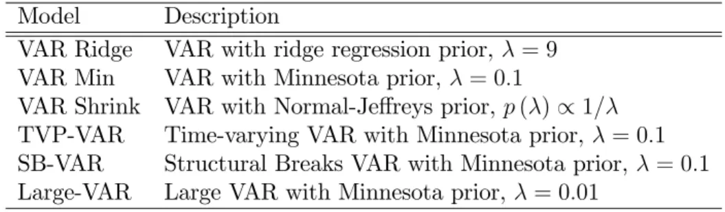
Here I provide a summary of all the models presented in the previous section. The models compared in this article are the linear Bayesian VAR with ridge regression (VAR Ridge), Minnesota (VAR Min) and adaptive shrinkage prior (VAR Shrink). The two nonlinear models estimated for the UK data are the time-varying para-meters VAR (TVP-VAR) and the structural breaks VAR (SB-VAR), both with a Minnesota prior on the mean coecients8. Additionally a 13-variable linear VAR
with Minnesota prior is estimated (Large-VAR). The variables in this model are the ones used in the trivariate VARs above plus 10 major variables for the UK economy including GDP, total employment, £/$ exchange rate and money stock M4 . These models are summarized in Table 1. This gives forecasts from six models with and without variable selection, i.e. a total of 12 model forecasts to assess. All models have an intercept and 4 lags of the dependent variables.
Moreover, we have to decide on selection of the shrinkage coecient for the Minnesota prior. This can be done subjectively as in Litterman (1986), but also searching over a grid of values in a training sample as in Ba´nbura, Giannone and Reichlin (2010). A value of = 0.1 is used for the trivariate linear and nonlin-ear VARs. This choice is the one which optimizes the forecasting performance of the TVP-VAR model in particular, compared to competing values of in the grid
{1,0.5,0.1,0.01,0.01}. Note that this “sensitivity analysis” approach is done be-cause the main purpose of this section is to evaluate the performance of variable selection and not which of the various VARs performs the best. It turns out that for the whole grid of values for , the conclusions about whether including variable selection improves forecasting or not are qualitatively similar. Following the same procedure, and based on the arguments of Ba´nbura, Giannone and Reichlin (2010),
8A “less tight” ridge regression prior can also be used in the initial condition of the mean
coef-ficients of these two models, say0Nn(0,9I). In that case, variable selection indeed performs
much better than no variable selection. In practical situations though, one would realistically use a data-based shrinkage prior in these models (like the Minnesota or the Primiceri, 2005, prior) to reduce the nonlinear parameter space.
who compare VARs of large dimensions, the shrinkage factor on the large linear VAR model is set to a tighter value, i.e. = 0.01.
Table 1: Definition of VAR models for the UK macro series Model Description
VAR Ridge VAR with ridge regression prior,= 9 VAR Min VAR with Minnesota prior,= 0.1
VAR Shrink VAR with Normal-Jereys prior,p()1/
TVP-VAR Time-varying VAR with Minnesota prior,= 0.1 SB-VAR Structural Breaks VAR with Minnesota prior,= 0.1 Large-VAR Large VAR with Minnesota prior,= 0.01
4.2
Forecast implementation
The initial estimation period is 1971Q1 to 1989Q4 and forecasts are computed iter-atively forhquarters ahead,h= 1,2,3,4. Then one data point is added at the end of the sample (1990Q1) and forecasting is implemented again for hquarters ahead. This procedure is followed until the sample is exhausted. Estimation is based on 30.000 samples from the posterior after an initial convergence (burn-in) period of 2.000 iterations. Convergence of the Gibbs sampler is excellent in all instances.
Standard results for forecasting with VAR models apply whether or not variable selection is present. The companion form of the standard VAR model is
yt =c+Byt1+t where yt = yt, ..., ytp+1,t = (t,0, ...,0), c= (c,0, ...,0) and B= B1...Bp1 Bp Im(p1) 0m(p1)m .
Iteratedh-step ahead forecasts can be computed using the formulas E(yt+h) = h1 i=0 B ic+Bhy t1 var(yt+h) = h1 i=0 B i(Bi) (20)
Two points have to be clarified here. First, in the case of variable selection, the parameter matricesB1, ..., Bp are going to be replaced by the respective elements of
the restricted parameter vector=. Second, in the case of the two models with drifting coecients, predictive simulation can be implemented to forecast breaks in the coecients out-of-sample. This would mean that we should use the random walk evolution of the mean coecients in the time-varying parameters and structural breaks VARs and simulate their future path using Monte Carlo; see Bauwens, Koop, Korobilis and Rombouts (2011) for more details. I follow D’Agostino, Gambetti and Giannone (2010) and relax this assumption. In that case, I use the formula (20) where I plug-in the last known values of the coecients in sample, i.e. T and s
T respectively for the two nonlinear models.
Using MCMC implies that we sample from the full posterior density of the VAR coecients, so that instead of a single point forecast E(yt+h) we end up having
samples from the full Bayesian predictive density. This also implies that there are two ways to implement the variable selection forecasts. The one is to estimate a specific VAR model using the Gibbs sampler, save the sequence of S = 30.000 posterior draws s, s = 1, ..., S, and obtain the mean/median . Then the “best”
model is the one for which j is unrestricted (restricted) if 0.5 ( < 0.5), so that we can estimate and forecast only with this best model at a second step. The second way is simply to implement one run of the MCMC and forecast using the current estimates s=ss fors= 1, ..., S MCMC samples. That way if we sample
j = 1 10% of the time (3.000 samples from the posterior) and j = 0 for the remaining samples, this means that we also use j to produce the final forecasts only 10% of the time. The former case provides absolute variable selection of a single optimal model, which is what Barbieri and Berger (2004) call the “median probability model”. The second method provides relative variable selection which is equivalent to Bayesian Model Averaging. In previous research (Korobilis, 2008; Koop and Korobilis, 2009) I find that there is no clear dominance of one method over the other in forecasting. In face of this result, I use the second method for forecasting which takes explicitly into account uncertainty about the true model (by giving relative, instead of absolute, weights to each VAR coecient).
4.3
Forecast evaluation
All models are evaluated using various measures of out-of-sample performance and forecast accuracy. Precision of mean forecasts is evaluated using averages of the Mean Absolute Forecast Error (MAFE) and the Root Mean Squared Forecast Error (RMSFE) over the whole pseudo out-of-sample evaluation period. In particular, for each of the three variables yi,t (i =inflation, unemployment, interest rate) of the
vector yt, and conditional on the forecast horizon h and the time period t, these
three measures are calculated as
M AF Eh i = 1 1h0+ 1 1h t=0 yi,t+h|tyi,to+h RM SF Eh i = 1 1h0+ 1 1h t=0 yi,t+h|tyi,to+h 2
where yi,t+h|t is the timet+hprediction of variablei, made using data available up
to timet, andyo
i,t+h is the observed out-of-sample value (realization) of variableiat
time t+h. In the recursive forecasting exercise, averages over the full forecasting period 1990:Q1 - 2008:Q4 are presented using these formulas where 0 is 1989:Q4 and 1 is 2008:Q4.
These two measures can help provide a ranking of all the VAR models and give an idea of which model and prior specification performs the best. An interesting question to answer is whether the inclusion of variable selection results in overall im-provement of forecasts. A simple measure is to compute the time series of dierences between the squared losses of the two models, i.e.
dt+h=
Rt+h2Ut+h2, (21)
whereRt 2 are the squared forecast errors from the restricted model (with variable selection), and U
t+h
2
are the squared forecast errors from the unrestricted model (without variable selection). The subscripttruns only for the pseudo out-of-sample period 1h0+ 1. Diebold and Mariano (1995) provide a simple test statistic when the null is that of equal predictive ability, i.e. E(dt+h) = 0. From a Bayesian
point of view, since we have 30.000 samples from the predictive density of our data yt+h, it is easy to construct through equation (21) an equal number of samples from
the finite sample density of dt+h. Hence this Bayesian procedure is equivalent, but
not identical, to bootstrapping dt under the assumption of Gaussianity (instead of
having to rely on the asymptotic distribution ofdt in the presence of small samples).
Subsequently, it is straightforward to get a pairwise measure of overall predictive ability by using the whole posterior density Pr (dt+h), i.e. we can evaluate the
following “Bayesian Diebold-Mariano” (BDM) statistic
BDM = 1
1h0+ 1
1h
t=0
Pr (dt+h>0), (22)
see also Garratt, Koop, Mise and Vahey (2009). This statistic implies that if BDM > 0.5, the unrestricted model performs better than the restricted model, and vice versa.
4.4
In-sample variable selection results
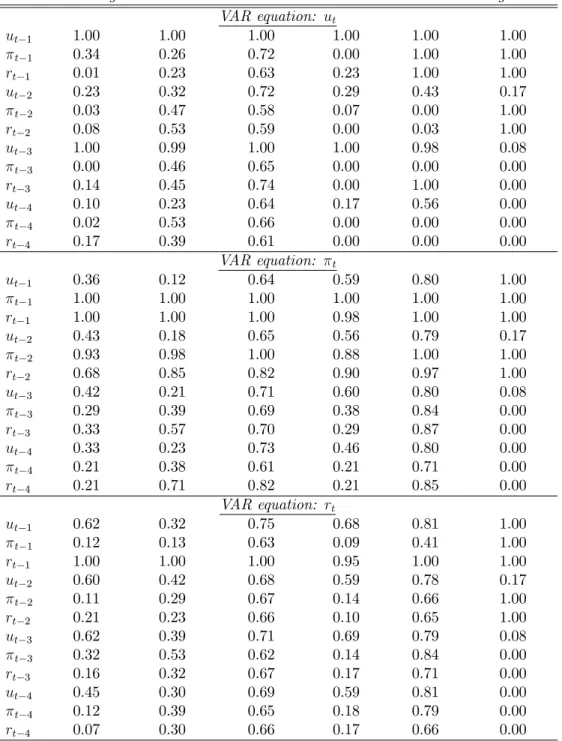
Before proceeding to the forecast evaluation of variable selection, it would be inter-esting first to obtain a picture of what is the output of variable selection. Since the Gibbs sampler provides a sequence of 0-1 draws from the posterior of, once we take an average of these draws we can end up with an average “probability of inclusion in the true model” for the respective VAR coecients. Table 2 does exactly that for the six models described earlier. The table is split in three blocks pertaining to each of the three VAR equations (unemployment ut, inflation t and interest rate
rt). Each row corresponds to the lags of the three variables as they appear in each
equation. Numerical entries in this table are the averages of the posterior of using the full sample 1971:Q1 - 2008:Q4. The prior on for the five trivariate VARs is the Bernoulli(0.8) discussed earlier, whilst for the Large VAR model the tighter prior discussed in subsection 3.4 applies.
Variable selection indicates that some variables should always be included, irre-spective of the model specification or the priors used. These are the first own lags of each dependent variable, but also the first lag of the interest rate in the inflation equation. Moreover, inflation and interest rates two periods ago seem to aect the
Table 2: Posterior means of the restriction variablesj using the full sample
VAR Ridge VAR Min VAR Shrink SB-VAR TVP-VAR Large-VAR
VAR equation: ut ut1 1.00 1.00 1.00 1.00 1.00 1.00 t1 0.34 0.26 0.72 0.00 1.00 1.00 rt1 0.01 0.23 0.63 0.23 1.00 1.00 ut2 0.23 0.32 0.72 0.29 0.43 0.17 t2 0.03 0.47 0.58 0.07 0.00 1.00 rt2 0.08 0.53 0.59 0.00 0.03 1.00 ut3 1.00 0.99 1.00 1.00 0.98 0.08 t3 0.00 0.46 0.65 0.00 0.00 0.00 rt3 0.14 0.45 0.74 0.00 1.00 0.00 ut4 0.10 0.23 0.64 0.17 0.56 0.00 t4 0.02 0.53 0.66 0.00 0.00 0.00 rt4 0.17 0.39 0.61 0.00 0.00 0.00 VAR equation: t ut1 0.36 0.12 0.64 0.59 0.80 1.00 t1 1.00 1.00 1.00 1.00 1.00 1.00 rt1 1.00 1.00 1.00 0.98 1.00 1.00 ut2 0.43 0.18 0.65 0.56 0.79 0.17 t2 0.93 0.98 1.00 0.88 1.00 1.00 rt2 0.68 0.85 0.82 0.90 0.97 1.00 ut3 0.42 0.21 0.71 0.60 0.80 0.08 t3 0.29 0.39 0.69 0.38 0.84 0.00 rt3 0.33 0.57 0.70 0.29 0.87 0.00 ut4 0.33 0.23 0.73 0.46 0.80 0.00 t4 0.21 0.38 0.61 0.21 0.71 0.00 rt4 0.21 0.71 0.82 0.21 0.85 0.00 VAR equation: rt ut1 0.62 0.32 0.75 0.68 0.81 1.00 t1 0.12 0.13 0.63 0.09 0.41 1.00 rt1 1.00 1.00 1.00 0.95 1.00 1.00 ut2 0.60 0.42 0.68 0.59 0.78 0.17 t2 0.11 0.29 0.67 0.14 0.66 1.00 rt2 0.21 0.23 0.66 0.10 0.65 1.00 ut3 0.62 0.39 0.71 0.69 0.79 0.08 t3 0.32 0.53 0.62 0.14 0.84 0.00 rt3 0.16 0.32 0.67 0.17 0.71 0.00 ut4 0.45 0.30 0.69 0.59 0.81 0.00 t4 0.12 0.39 0.65 0.18 0.79 0.00 rt4 0.07 0.30 0.66 0.17 0.66 0.00
current level of inflation, as well as the third lag of unemployment aects the cur-rent level of unemployment (but only in the small, trivariate VAR models). Lastly, unemployment in the previous quarter is more likely to aect the current level of the interest rate than past inflation.
Other than these few regularities, the posterior probabilities of inclusion of each predictor variable varies a lot between specifications. For the linear VAR model, the relatively uninformative ridge regression prior invites more restrictions from the vari-able selection algorithm than when the Minnesota and Normal-Jerey’s priors are present. This is because the last two priors already provide shrinkage of coecients towards zero. Subsequently it is the case that shrinkage will force more (compared to an uninformative prior) the posterior of the j’s to move towards the region of zero, so that the respective j’s are not identified and they will be drawn randomly from theirBernoulli(0.8)prior. As discussed earlier, this is not a failure of variable selection since what we care about is the combined coecient j = jj to be zero,
whether it is becausej = 0or j = 0. An example where this eect happens is for variablet2 in the unemployment equation, which has only a probability of 8% of inclusion when using the VAR Ridge model, but this probability increases to circa 50% when using the VAR Min and VAR Shrink models. Nevertheless, in these two latter models, the posterior mean ofj forj =t2is around 0.002, so that it finally holds that j =jj 0.
For the rest of the VAR models mixed results are present which depend on the nature of each model. Even among the two nonlinear models many dierences exist. For instance,t1has 0% probability of appearing in the unemployment equation of the structural breaks VAR but 100% probability of appearing in the same equation in the time-varying VAR model. Finally, notice that more restrictions are present in the Large-VAR model since a more restricted form of the prior onis used, compared to the one used in the small models. In this Large-VAR setting the right-hand side (RHS) variables have exactly the same probability of appearing in each of the three VAR equations of interest. This is due to the simplifying assumption described in subsection 3.4 which allows computational tractability when the dimensions of the VAR grow large.
4.5
Out-of-sample iterated forecasts
In this subsection the restricted and unrestricted VAR models are evaluated out-of-sample. Tables 3 and 4 present the MAFE and RMSFE statistics over the forecast sample 1990:Q1-2008:Q4. The first column of each table shows the three variables in the vector of interestyt+h, for horizonsh= 1, ...,4. The second column of both tables
presents the absolute value of the MAFE and RMSFE, respectively, for the driftless random walk model. Consequently the remaining columns present the MAFE and RMSFE statistics from the six Bayesian four-lag VARs with and without variable selection, as a proportion of the respective MAFE and RMSFE of the random walk. For comparison the third column in each table gives the respective statistics from a parsimonious VAR(1) specification estimated with OLS.
The results suggest that all small four-lag VAR models perform better the naïve model in short-term forecasting of unemployment and inflation. The very flexi-ble TVP-VAR provides the lowest mean prediction error (the gains are especially visible during the financial crisis sample 2007-2008), while the Large VAR being quite heavily parametrized gives only the best VAR forecasts for the interest rate. Nevertheless, none of the VAR models can beat the random walk in interest rate forecasting.
In terms evaluating variable selection, the unrestricted VAR(4) model with ridge regression prior (which in this paper is defined to be uninformative, as if using a VAR(4) estimated with least squares) is better at all horizons than the unrestricted, more parsimonious VAR(1) in forecasting unemployment and inflation. In that respect, good performance of the variable selection is translated into expecting sub-stantial restrictions of the VAR(4) Ridge model coecients only in the interest rate equation since from the VAR(1) it is obvious that using one lag in this equation is always better. At the same time less restrictions are expected in the coecients in the unemployment and interest rate equation, since the VAR(4) is already doing much better than the VAR(1) for these two equations. Table 2 provided an idea of the restrictions that actually hold in each model, however notice that in a recur-sive forecasting exercise the posterior probabilities are estimated in real-time as new data become available, so they will not be constant during the forecast evaluation sample.
Ta b le 3 : R el a ti v e M A F E o f u n re st ri ct ed a n d re st ri ct ed V A R s: u n em p lo y m en t, in fl a ti o n a n d in te re st ra te fo r h =1 , 2 , 3 an d 4 . RW V A R (1 ) VA R (4 ) R id ge VA R (4 ) M in VA R (4 ) S h ri n k S B -VA R (4 ) T V P -VA R (4 ) L a rg e-V A R (4 ) MA F E O L S n o V S w it h V S n o V S w it h V S n o V S w it h V S n o V S w it h V S n o V S w it h V S n o V S w it h V S ut+1 0. 1 34 3 1. 0 7 0. 88 0. 88 0. 87 0. 86 0. 86 0. 86 0. 88 0. 86 0. 84 0. 84 0. 95 0. 8 6 t+1 0. 4 88 2 1. 1 8 0. 91 0. 88 0. 90 0. 88 0. 88 0. 89 0. 90 0. 90 0. 83 0. 83 1. 24 1. 2 1 rt+1 0. 4 04 7 1. 3 1 1. 45 1. 45 1. 43 1. 44 1. 42 1. 41 1. 36 1. 33 1. 33 1. 33 1. 22 1. 1 7 ut+2 0. 2 16 3 1. 1 4 0. 94 0. 92 0. 93 0. 93 0. 92 0. 91 0. 94 0. 86 0. 83 0. 84 1. 03 0. 9 0 t+2 0. 8 17 3 1. 2 4 1. 00 1. 00 0. 96 0. 97 1. 00 1. 02 0. 97 1. 01 0. 86 0. 88 1. 36 1. 2 9 rt+2 0. 6 97 1 1. 3 8 1. 59 1. 55 1. 57 1. 52 1. 50 1. 47 1. 50 1. 47 1. 39 1. 37 1. 09 1. 0 1 ut+2 0. 2 91 2 1. 1 5 0. 96 0. 92 0. 95 0. 94 0. 93 0. 92 0. 95 0. 87 0. 79 0. 81 1. 12 0. 9 1 t+3 1. 1 01 4 1. 3 5 1. 18 1. 16 1. 12 1. 09 1. 13 1. 14 1. 15 1. 11 0. 88 0. 91 1. 64 1. 5 3 rt+3 0. 9 53 2 1. 4 5 1. 74 1. 64 1. 70 1. 60 1. 55 1. 51 1. 63 1. 46 1. 47 1. 41 1. 06 1. 0 3 ut+4 0. 3 47 9 1. 1 6 0. 99 0. 95 0. 99 0. 98 0. 97 0. 96 0. 99 0. 88 0. 80 0. 83 1. 22 0. 9 3 t+4 1. 2 86 3 1. 5 1 1. 49 1. 46 1. 40 1. 34 1. 37 1. 37 1. 46 1. 45 1. 02 1. 01 1. 91 1. 7 7 rt+4 1. 1 86 8 1. 5 2 1. 79 1. 70 1. 74 1. 65 1. 58 1. 54 1. 68 1. 49 1. 49 1. 44 1. 10 1. 0 4 No t e : T h e s e c o n d c o lu m n s h o w s t h e a b s o lu t e M AF E o f t h e R a n d o m W a lk ( R W ) . R e m a in in g c o lu m n s r e p o r t M AF E s o f e a c h V AR m o d e l r e la t iv e t o t h e M A F E o f t h e R W . No VS / w it h VS in d ic a t e s t h e p r e s e n c e o f v a r ia b le s e le c t io n . Ta b le 4 : R el a ti v e R M S F E o f u n re st ri ct ed a n d re st ri ct ed V A R s: u n em p lo y m en t, in fl a ti o n a n d in te re st ra te fo r h =1 , 2 , 3 an d 4 . RW V A R (1 ) VA R (4 ) R id ge VA R (4 ) M in VA R (4 ) S h ri n k S B -VA R (4 ) T V P -VA R (4 ) L a rg e-V A R (4 ) MA F E O L S n o V S w it h V S n o V S w it h V S n o V S w it h V S n o V S w it h V S n o V S w it h V S n o V S w it h V S ut+1 0. 1 71 2 1. 0 7 0. 85 0. 84 0. 84 0. 84 0. 83 0. 83 0. 85 0. 85 0. 79 0. 80 0. 92 0. 8 6 t+1 0. 6 82 8 1. 1 0 0. 85 0. 84 0. 85 0. 86 0. 87 0. 88 0. 85 0. 89 0. 79 0. 80 1. 13 1. 1 1 rt+1 0. 6 37 8 1. 1 6 1. 24 1. 25 1. 23 1. 23 1. 24 1. 23 1. 17 1. 23 1. 16 1. 18 1. 07 1. 0 4 ut+2 0. 2 93 3 1. 0 4 0. 84 0. 81 0. 83 0. 82 0. 82 0. 81 0. 83 0. 81 0. 75 0. 77 0. 91 0. 8 4 t+2 1. 1 15 7 1. 2 2 0. 95 0. 96 0. 93 0. 94 0. 97 0. 98 0. 93 1. 03 0. 80 0. 81 1. 26 1. 1 9 rt+2 1. 0 27 8 1. 2 3 1. 37 1. 33 1. 34 1. 32 1. 30 1. 29 1. 29 1. 28 1. 24 1. 24 1. 00 0. 9 3 ut+2 0. 4 04 7 1. 0 0 0. 85 0. 81 0. 84 0. 83 0. 82 0. 81 0. 84 0. 81 0. 73 0. 76 0. 99 0. 8 4 t+3 1. 4 59 6 1. 3 7 1. 16 1. 16 1. 12 1. 10 1. 12 1. 13 1. 13 1. 08 0. 89 0. 91 1. 55 1. 4 7 rt+3 1. 3 44 1 1. 2 8 1. 47 1. 40 1. 43 1. 37 1. 34 1. 32 1. 39 1. 29 1. 30 1. 30 1. 00 0. 9 9 ut+4 0. 4 98 6 0. 9 6 0. 82 0. 79 0. 82 0. 81 0. 80 0. 79 0. 82 0. 79 0. 70 0. 73 1. 05 0. 8 3 t+4 1. 7 03 6 1. 5 4 1. 44 1. 42 1. 37 1. 32 1. 33 1. 33 1. 41 1. 41 1. 03 1. 03 1. 83 1. 7 2 rt+4 1. 6 40 6 1. 3 1 1. 49 1. 43 1. 46 1. 40 1. 36 1. 33 1. 41 1. 30 1. 31 1. 28 1. 03 1. 0 2 No t e : T h e s e c o n d c o lu m n s h o w s t h e a b s o lu t e M AF E o f t h e R a n d o m W a lk ( R W ) . R e m a in in g c o lu m n s r e p o r t M AF E s o f e a c h V AR m o d e l r e la t iv e t o t h e M A F E o f t h e R W . No VS / w it h VS in d ic a t e s t h e p r e s e n c e o f v a r ia b le s e le c t io n .
In fact, variable selection in the VAR(4) Ridge model does improve forecasts of all three variables, especially at longer horizons. For the VAR(4) Min and VAR(4) Shrink (these two models already have shrinkage priors) variable selection only im-proves the interest rate forecast while there is usually a±1% gain/loss in MAFE or RMSFE, but this is so small that might also be attributed to sampling and rounding error. The main result is that none of the three unrestricted linear VARs with four lags is forecasting interest rates as the VAR(1) estimated with OLS does, something that is consistently accounted for when adding variable selection9.
The gains from variable selection for forecasting all three variables of interest are more clear as the model size increases. As forecasting results for the 13-variable Large VAR suggest, when the model dimensions increase, variable selection really helps to prevent overfitting. Although the Minnesota shrinkage parameter is not set optimally, this improvement when using variable selection is robust for a large grid of values of (see the discussion in subsection 4.1).
The story behind the structural breaks model SB-VAR(4) is dierent. There, the gains are quite impressive for longer horizons, but closer examination shows that these are linked only indirectly to variable selection. Estimation of the unrestricted SB-VAR(4) model with maximum number of possible breaks equal to 3, indicates that there are actually no breaks10. When the SB-VAR(4) model is estimated with variable selection, a break is found (using the full sample) in 2004Q1. This is actually the exact reason why variable selection does much better in mean prediction with the structural breaks model. By restricting the parameter space, a structural break is found that is not otherwise identified when all 39 mean VAR coecients are unrestricted.
In the TVP-VAR model with Minnesota prior, which is the best performing among all VAR models, variable selection helps improve the MAFE of the interest
9Here we can observe that although variable selection improves forecasts of interest rate from
the linear VAR(4), these are never as good as the VAR(1)-OLS forecasts. This is due to the fact that our prior expection is that 20% of the parameters should be restricted (0j = 0 = 0.8).
Subsequently there might be benefit from setting 0j<<0.8but only if j is a coecient in the
interest rate equation; see also the discussion in the next subsection.
10Notice that although no breaks are estimated, the SB-VAR(4) forecasts are not the same
as the VAR(4) Min forecasts (these two models have identical Minnesota priors). The reason is computational, but explaining why is beyond the scope of this paper. The reader is advised to consult Bauwens, Koop, Korobilis and Rombouts (2011).
rate in longer horizons. Nevertheless, in this case variable selection increases the absolute and squared forecast error of unemployment and inflation at horizons two to four quarters. Subsequently, the shrinkage prior in this case is sucient to guar-antee optimal mean forecasts, and variable selection is not necessary. Although this observation might be correct for the expected risk of mean forecasts, the Bayesian Diebold-Mariano (BDM) statistic given in equation (22) reveals that there is the case that variable selection provides overall superior predictive ability.
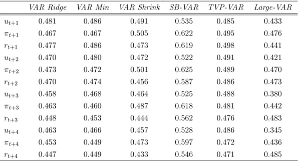
The BDM statistic, which is based on the time series of dierences between the squared forecast errors of the restricted and the unrestricted models, is presented in Table 5. A value less than 0.5 shows the probability that the restricted model has better forecasting ability overall compared to the unrestricted model. Table 5 reveals that this is the case for all models apart from the structural breaks VAR. That is because in this model we saw that variable selection indicates one break, while in the unrestricted model no break is found. Thus forecasts from the restricted model with one break have larger variance because all the VAR coecients in the second regime are estimated using only 19 observations (the break date is 2004Q1). Since the BDM statistic is based on all simulated draws from the posterior predictive densities, parameter uncertainty is included in the evaluation of the quantity Pr (dt+h >0).
Thus, this fact explains why the unrestricted no-break model does better overall than the restricted model with one break, despite the fact that the MAFE and RMSFE results suggest otherwise. Finally, in Table 5 we can observe again that as the forecast horizon increases the gains from using variable selection also increase.
Table 5: Bayesian Diebold-Mariano statistic, T1 Pr (dt+h>0).
VAR Ridge VAR Min VAR Shrink SB-VAR TVP-VAR Large-VAR
ut+1 0.481 0.486 0.491 0.535 0.485 0.433 t+1 0.467 0.467 0.505 0.622 0.495 0.476 rt+1 0.477 0.486 0.473 0.619 0.498 0.441 ut+2 0.470 0.480 0.472 0.522 0.491 0.421 t+2 0.473 0.472 0.501 0.625 0.489 0.470 rt+2 0.470 0.474 0.456 0.587 0.486 0.473 ut+3 0.458 0.468 0.464 0.525 0.488 0.380 t+3 0.463 0.460 0.487 0.618 0.481 0.442 rt+3 0.448 0.453 0.444 0.562 0.476 0.483 ut+4 0.463 0.466 0.457 0.528 0.486 0.345 t+4 0.453 0.449 0.473 0.597 0.472 0.436 rt+4 0.447 0.449 0.433 0.546 0.471 0.485
N o t e : T h e Ta b le s h ow s th e ave ra g e va lu e s o f th e s ta t is tic P r(dt + h>0 ) w h e redt + h a re t h e tim e s e rie s o f d ie re n c e s b e tw e e n t h e s q u a re d fo re c a s t e rro rs fro m th e re s t ric t e d a n d u n re s tric t e d m o d e ls ; s e e a ls o e q u a t io n (2 2 ) in th e te x t .
4.6
Sensitivity analysis: Direct forecasts, and expected
num-ber of restrictions
In many cases, iterated, multi-step ahead VAR forecasts might not be satisfactory. This is particularly true when the model is misspecified (Marcellino, Stock and Wat-son, 2006), in which case econometricians estimate a direct VAR using information up to time tto directly predict yt+h, i.e. the model
yt+h =Bxt+t.
Using the above VAR equation, the researcher can use directly the available infor-mation xT to forecast yT+h. This is, additionally, a particularly useful approach
when xt contains exogenous predictors for which forecasts are not available to the
econometrician (and hence iterating the VAR h-steps ahead is not possible). This case is examined analytically in Korobilis (2008) using the SSVS algorithm in large linear VARs with hundreds of predictors. Here I provide results for 4-steps ahead forecasting using the TVP-VAR(4) in the context of a “sensitivity analysis”
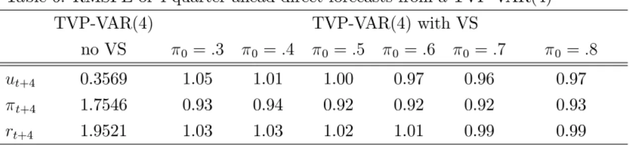
with varying degree of prior expected number of restrictions. Restrictions in the VAR models with variable selection can be imposed through the prior hyperpara-meter 0j of the Bernoulli density in equation (6). Table 6 presents the RMSFE
from the unrestricted TVP-VAR(4) in the second column, and the RMSFE of the restricted TVP-VAR(4) with 0j = 0 for all j = 1, ..., n, relative to that of the unrestricted model. The case 0 = 0.8 is the one examined previously in the small VARs (but it was relaxed in the Large VAR model) and implies the expectation that 20% of the coecients should be restricted a priori. Other values shown in this Table can be interpreted in a similar way. The optimal forecasts from the re-stricted model are obtained when 0 is 0.7, where gains of up to 8% in forecasting inflation are attained. When more and more restrictions are imposed, the RMSFE are monotonically increasing, suggesting that there is a risk attached to imposing strong prior beliefs in such a small model. For 0 >0.7 the RMSFE also increases, where the limit 0 = 1implies the unrestricted model (where all relative RMSFEs are equal to 1.00).
Table 6: RMSFE of 4-quarter ahead direct forecasts from a TVP-VAR(4)
TVP-VAR(4) TVP-VAR(4) with VS
no VS 0 =.3 0 =.4 0 =.5 0 =.6 0 =.7 0 =.8 ut+4 0.3569 1.05 1.01 1.00 0.97 0.96 0.97 t+4 1.7546 0.93 0.94 0.92 0.92 0.92 0.93 rt+4 1.9521 1.03 1.03 1.02 1.01 0.99 0.99
N o t e : T h e s e c o n d c o lu m n p re s e nts t h e R M S F E o f th e u n re s tric t e d T V P -VA R ( 4 ) m o d e l. T h e n e x t c o lu m n s p re s e nt t h e R M S F E s o f t h e re s tric t e d m o d e l ( re la tive t o t h a t o f th e u n re s tric t e d T V P -VA R ( 4 )) fo r d ie re nt p rio r e x p e c t e d nu m b e r o f re s tric t io n s o n.
Although for other direct VAR models and forecast horizons results are mixed as to whether variable selection improves forecasting over the unrestricted model, it is always the case that for small VAR models the RSMFE is a quadratic function of0. Consequently, choice of0 should not pose a challenge for the applied researcher as soon as the choice of expected restrictions is chosen reasonably, i.e. it is tied to the dimension of the VAR model considered. For instance, in subsection 3.4 an empirical method for tuning the prior expected number of restrictions as the dimension of the VAR increases was introduced. Moreover, if there are actually practical diculties
in selecting a value for 0, full Bayes methods can also be used. That means that a hyperpior distribution is placed on 0 (or even 0j for j = 1, ..., n), so that this
hyperparameter is estimated from the data and hence it will also vary with the sample size considered.
5
Concluding remarks
Vector autoregressive models have been used extensively over the past for the pur-pose of macroeconomic forecasting, since they have the ability to fit the observed data better than competing theoretical and large-scale structural macroeconometric models. This paper shows that Bayesian variable selection methods can be used to find restrictions based on the evidence in the data with positive implications in preserving parsimony. It was argued that these types of restrictions are important for long-horizon forecasts as well as forecasts from large VAR systems. Specifically, variable selection i) dominates forecast from VAR models with uninformative priors; ii) competes favourably to shrinkage estimation; and iii) provides more benefits in forecasting as the model size increases.
References
Ba´nbura, M., Giannone, D. and Reichlin, L. (2010). Large Bayesian vector auto regressions. Journal of Applied Econometrics, 25, 71-92.
Barbieri, M. M., and J. O. Berger. (2004). Optimal predictive model selection. The Annals of Statistics, 32, 870-897.
Bauwens, L., Koop, G., Korobilis, D., and J. Rombouts. (2011). A compari-son of forecasting procedures for macroeconomic series: The contribution of structural break models. CIRANO Working Papers 2011s-13, CIRANO. Canova, F. (1993). Modelling and forecasting exchange rates using a Bayesian time
varying coecient model. Journal of Economic Dynamics and Control,17, 233-262.
Canova, F., and L. Gambetti. (2009). Structural changes in the US economy: Is there a role for monetary policy? Journal of Economic Dynamics and Control, 33, 477-490.
Carter, C., and R. Kohn (1994). On Gibbs sampling for state space models. Bio-metrika, 81, 541-553.
Chan, J. C. C., Koop, G., Leon-Gonzalez, R., and Strachan, R. W. (2010). Time-varying dimension models. ANU School of Economics Working Papers 2010-523.
Chib, S. (1996). Calculating posterior distributions and modal estimates in Markov mixture models. Journal of Econometrics, 75, 79-98.
Chipman, H., George, E. I., and R.E. McCulloch. (2001). The practical imple-mentation of Bayesian model selection. In P. Lahiri (Ed.), Model Selection, (pp. 67-116). IMS Lecture Notes — Monograph Series, vol. 38.
Cogley, T., Morozov, S., and T. Sargent. (2005). Bayesian fan charts for U.K. infla-tion: Forecasting and sources of uncertainty in an evolving monetary system. Journal of Economic Dynamics and Control, 29, 1893-1925.
Cogley, T., and T. Sargent. (2002). Evolving post-World War II inflation dynam-ics. NBER Macroeconomics Annual, 16, 331-388.
Clark, T. E., and M. W. McCracken. (2010). Averaging forecasts from VARs with uncertain instabilities. Journal of Applied Econometrics, 25, 5-29.
D’Agostino, A., Gambetti, L., and D. Giannone. (2009). Macroeconomic forecast-ing and structural change. ECARES Workforecast-ing Paper 2009-020.
Diebold, F. X. and R. S. Mariano. (1995). Comparing predictive accuracy. Journal of Business and Economic Statistics, 13, 253-263.
Doan, T., R. Litterman, and C. A. Sims. (1984). Forecasting and conditional projection using realistic prior distributions. Econometric Reviews, 3, 1-100.