Itemset Mining
Siegfried Nijssen and Tias Guns
K.U. Leuven, Celestijnenlaan 200A, B-3001 Leuven, Belgium {Siegfried.Nijssen, Tias.Guns}@cs.kuleuven.be
Abstract. Over the years many pattern mining tasks and algorithms have been proposed. Traditionally, the focus of these studies was on the efficiency of the computation and the scalability towards very large databases. Little research has however been done on a general framework that encompasses several of these problems. In earlier work we showed how constraint programming (CP) can offer such a general framework; unfortunately, however, we also found that out-of-the-box CP solvers lack the efficiency and scalability achieved by specialized itemset mining systems, which could discourage their use. Here we study the question whether a framework can be built that inherits the generality of CP sys-tems and the efficiency of specialized algorithms. We propose a CP-based framework for pattern mining that avoids the redundant representations and propagations found in existing CP systems. We show experimentally that an implementation of this framework performs comparable to spe-cialized itemset mining systems; furthermore, under certain conditions it lists itemsets with polynomial delay, which demonstrates that it also is a promising approach for analyzing pattern mining tasks from more theoretical perspectives. This is illustrated on a graph mining problem.
1
Introduction
Constraint-based pattern mining is a topic that has been studied extensively. Popular examples are frequent and closed itemset mining [1, 16, 11, 9, 7, 15], but also more general constraints have been studied [10, 6, 4]. Patterns can be used directly, or may serve as an intermediate step when building classifiers or com-pressing data, in which case additional constraints can be imposed.
The main focus of most studies on pattern mining is on how to efficiently com-pute the set of solutions, given a specific set of constraints. The frequent itemset mining implementation challenge (FIMI [9]) was organized to fairly compare the runtime efficiency and memory consumption of different algorithms that were proposed over the years. An overwhelming number of aspects have been stud-ied, ranging from algorithmic aspects, such as breadth-first or depth-first search; data structures, such as using row-oriented (horizontal), column-oriented (ver-tical), or tree-based representations; as well as implementation aspects, such as the most efficient way to represent sets and count their cardinality.
An issue which received considerably less attention is howgenerally applica-ble some of the algorithms and their proposed optimizations are. Indeed, even
though a number of systems have been developed which support multiple con-straints (see [10, 6, 7, 4], for instance), usually the constraint language is limited to a small number of primitives that are hard-coded in the algorithm; no sup-port is provided for adding constraints other than post-processing the patterns. We proposed an alternative approach in previous work [8], which relies on the use of existing constraint programming systems. These are generally applicable constraint satisfaction solvers developed by the artificial intelligence community [13, 14]. They are commonly used to solve complex problems such as planning, scheduling and resource allocation. We showed that several well-known pattern mining problems can be modeled using constraint programming primitives. At the same time, however, we found that state-of-the-art CP systems often per-form an order of magnitude worse than well-known itemset mining algorithms on popular itemset mining tasks such as closed and frequent itemset mining. CP systems were only competitive on tasks characterized by a large number of restrictive constraints. This performance gap could become troublesome for very large datasets, as well as when using very low frequency thresholds. To make constraint programming a viable alternative to specialized algorithms, we believe that it is desirable that the performance gap is reduced.
In this paper we study this problem. We perform an analysis which shows that existing CP systems represent data in a highly redundant way and propagation —the key computational mechanism in CP systems— is more often performed than necessary. To address this problem, we propose several key changes in CP systems: (1) we propose to use representations of data common in data mining in CP; (2) we propose that propagators share these representations; (3) we propose a mechanism through which propagators can share inferred constraints with each other; this allows to eliminate redundant computations by the propagators.
The resulting system maintains the principles of CP systems while being far more efficient than out-of-the-box constraint solvers. In particular, we will show that our CP system also achieves polynomial delay on mining problems that were only recently shown to have such complexity [3, 2]; we show that CP provides an alternative framework for deriving algorithms of low computational complexity and illustrate this on a problem in graph mining. This observation is of interest as it shows that CP can be used as fundamental methodology for reasoning about data mining problems, including their computational complexity.
The paper is organized as follows. In Section 2 we summarize the problems of frequent itemset mining and constraint programming and their basic principles. In Section 3 we summarize our earlier work on modeling itemset mining in a CP framework and we identify the bottlenecks in current CP solvers by comparing them with traditional mining algorithms. In Section 4 we present our integrated approach to solving these problems. Section 5 analyses the theoretical complexity of our system while Section 6 studies it experimentally; Section 7 concludes.
2
Itemset Miners and CP Systems
Before we study how to integrate itemset miners and constraint programming systems, let us briefly summarize their basic principles.
2.1 Frequent Itemset Mining
Problem Formulation LetI={1, . . . , m} be a set of items, andT ={1, . . . , n} a set of transactions; an itemset databaseD is a binary matrix of sizen×m. Given such a database, we can define a function ϕ : 2I → 2T which maps an
itemset Ito a set of transactions as follows:
ϕ(I) ={t∈ T |∀i∈I:Dti= 1}. (1)
This set is called atid-set, denoted byT. Using the above function, the frequent itemset mining problem can be formulated as the problem of finding the set:
{(I, T) | I⊆ I, T ⊆ T, q(I, T)} where
q(I, T)⇔covers(I, T)∧f requent(I, T) (2)
covers(I, T)⇔(T =ϕ(I)) (3)
f requent(I, T)⇔(|T| ≥θ) (4)
andθ is theminimum frequencyparameter of the problem.
Variations of the frequent itemset mining problem include closed itemset mining, maximal itemset mining and itemset mining under monotonic or fault-tolerance constraints. In general, these can be thought of as alternative defini-tions ofq(I, T) that tuples (I, T) should satisfy.
Existing Algorithms Many algorithms have been proposed for the frequent item-set mining problem. We can distinguish three algorithmic choices: the search strategy, the representation of the data and of the sets.
Search strategy: the most well-known algorithm is the breadth-firstApriori algorithm [1]; an alternative search strategy is a depth-first search in which each node in the search tree corresponds to an itemset. The latter strategy is taken in most of the recent algorithms for reasons of memory efficiency.
Representation of the data: the itemset database D can be represented in three equivalent ways:
– as a binary matrix of sizen×m, having entriesDti;
– as a bag of n itemsets Dt, each of which represents a transaction with
Dt={i∈ I | Dti= 1}.This is referred to as ahorizontalrepresentation
of the binary matrix.
– as a bag of m tid-sets DT
i (one for each an item), where DT is the
transpose of matrixD. EachDT
i contains a set of transaction identifiers
such that DT
i = {t ∈ T | Dti = 1}. This is referred to as a vertical
representationof the binary matrix.
More complex representations also exist: FP-Growth [11], for instance, rep-resents the itemset database more compactly in a prefix-tree. We do not consider this representation here.
Algorithm 1Eclat(I,T,Ipos,D)
1: OutputI
2: Ipos′ =∅
3: for alli∈Ipos, i >max(I)do 4: if |T∩ DT i| ≥θthen 5: I′ pos:=Ipos′ ∪ {i} 6: end if 7: end for
8: for alli∈Ipos′ do 9: Eclat(I∪ {i},T∩ DT i,I ′ pos,D) 10: end for Algorithm 2Constraint-Search(D) 1: D:=propagate(D)
2: if D is a false domainthen 3: return 4: end if 5: if ∃v∈ V:|D(v)|>1then 6: v:= arg minv∈V,D(v)>1f(v) 7: Dp:= split(D(v)) 8: Constraint-Search(D∪ {v7→Dp}) 9: Constraint-Search(D∪ {v7→D−Dp}) 10: else 11: Output solution 12: end if
Representation of sets: tid-sets such asT andDT
i can be represented in
mul-tiple ways. One is asparse representation, consisting of a list of transaction identifiers included in the set (which is called apositive representation) or not included in the set (which is called anegative representation); the size of this representation changes as the number of elements in the set changes. The other is adense representation, in which case the set is represented as a boolean array. Large sets may require less space in this representation. A representative depth-first algorithm is theEclatalgorithm [16], which uses a vertical representation of the data; it can be implemented both for sparse and dense representations. The main observation which is used inEclatis the following: ϕ(I) =\ i∈I ϕ({i}) =\ i∈I DT i. (5)
This allows for a search strategy depicted in Algorithm 1. The initial call of this algorithm is for I =∅,T =T and Ipos =I. The depth-first search strategy is
based on the following properties. (1) If an itemset I is frequent, but itemset I∪ {i}is infrequent, all setsJ ⊇I∪ {i}are also infrequent. InIpos we maintain
those items which can be added to I and yield a frequent itemset. (2) If we add an item to an itemset, we can calculate the tid-set of the resulting itemset incrementally from the tid-set of the original itemset as follows: ϕ(I∪ {i}) = ϕ(I)∩ DT
i. (3) To avoid an itemset I from being generated multiple times, an
order is imposed on the items. We do not add items to an itemset I which are lower than the highest item already in the set.
2.2 Constraint Programming
Problem Formulation Constraint programming is a declarative programming paradigm for solving constraint satisfaction (CSP) and optimization problems. A CSP P= (V, D,C) is specified by
– a finite set of variablesV;
– an initial domainD(V) for every variable V ∈ V;
– a finite set of constraintsQ.
Aconstraintq(V1, . . . , Vk)∈ Qis a boolean function from variables{V1, . . . , Vk} ⊆
V. A domain usually consists of a finite set of values. A domain D′ is called
stronger than the initial domain D if D′(V) ⊆ D(V) for all V ∈ V; a
vari-able V ∈ V is called fixed if |D(V)|= 1. A solution to a CSP is a domain D′
that (1) fixes all variables (∀V ∈ V : |D′(V)| = 1) (2) satisfies all constraints
(∀q(V1, . . . , Vk)∈ Q : q(D′(V1), . . . , D′(Vk)) = 1); (3) is stronger than original
domainD(guaranteeing that every variable has a value from its initial domain). Existing Algorithms Most constraint programming systems perform depth-first search. A general outline is given in Algorithm 2 [14]. Branches of a node of the search tree are obtained by splitting the domain of a variable in two parts (line 7); for boolean variables, split({0,1})={0}or split({0,1})={1}. The search backtracks when a violation of constraints is found (line 2). The search is further optimized by carefully choosing the variable that is fixed next (line 6); a function f(V) scores each variable; the highest ranked is branched on. For instance,f(V) may count the number of constraints the variable is involved in.
The main concept used to speed-up the search is constraint propagation (line 1). Propagation reduces the domains of variables such that the domain remains consistent. In a consistent domain a valueddoes not occur in the domain of a variable V if it can be determined that there is no solution D′ in which D′(V) = {d}. This way, propagation effectively reduces the size of the search tree, avoiding backtracking as much as possible and hence speeding up the search. To maintain consistenciespropagatorsare used (sometimes also called prop-agation or filtering rules). A propagator takes as input a domain and outputs a stronger domain. For instance, for a constraintV < W withD(V) ={1,2}and D(W) = {1,4}, the propagator may output D(V) = {1,2} and D(w) ={4}. Propagation continues until a fixed point is reached in which the domain does not change any more.
A key ingredient of CP systems is that propagators are evaluated indepen-dently of each other; all communication between propagators occurs through the variables and, in some systems, by the insertion of (derived) constraints in the constraint store. This is what allows constraints to be combined and reused across different models.
There are many different CP systems; we identify the following differences:
Types of variables: the variables are at the core of the solver. Many solvers implement integer variables, of which the domains can be represented in two ways: representing every element in the domain separately or saving only the bounds of the domain, namely the minimum and maximum value the variable can still take.
Supported constraints: related to the types of variables, the supported con-straints determine the problems that can be modeled.
Propagator activation: a constraint is defined on a set of variables. When one of the variables’ domains changes, a propagator for the constraint needs
to be activated. A common strategy is to tell the propagator which domain changed (in CP, this strategy is known as AC-3); another strategy is to also tell the propagator how the domain changes (this strategy is known as AC-5 [13]). The latter strategy is useful to avoid activating propagators that cannot propagate certain variable assignments.
3
Frequent Itemset Mining in CP systems
We briefly summarize the CP formulation presented in our previous work [8]. We then study how CP solvers and itemset mining algorithms differ in the properties introduced in the previous section. In the next section we will use the best of both worlds to develop a new algorithm.
Problem Formulation To model itemset mining in a CP system, we use two sets of boolean variables:
– a variableIi for each itemi, which is 1 if the item is included in the solution
and 0 otherwise. The vectorI= (I1, . . . , Im) represents an itemset.
– a variableTt for each transaction t, which is 1 if the transaction is in the
solution and 0 otherwise. The vectorT = (T1, . . . , Tn) represents a tid-set.
A solution hence represents one itemsetIwith corresponding tid-setT. To find all frequent itemsets, we need to iterate over all solutions satisfying the following constraints: covers(I, T)⇔ ∀t∈ T :Tt= 1↔ X i∈I Ii(1− Dti) = 0. (6) f requent(I, T)⇔ ∀i∈ I:Ii= 1→ X t∈T TtDti≥θ. (7)
Constraint (6) is a reformulation of the constraint in equation (4); constraint (7) is derived from a combination of the original coverage and frequency constraints, as follows. We observe that in a solution (I, T): ∀i∈ I :|T|=|T∩ϕ({i})|, as T =ϕ(I)⊆ϕ({i}), and therefore that
∀i∈I:|T∩ϕ({i})| ≥θ⇐⇒ ∀i∈ I:Ii= 1→ X t∈T
TtDti≥θ.
Other well-known itemset mining problems can be formalized in a similar way. An overview is provided in Table 1; the correctness of these formulas was proved in [8]. The general type of constraint that we used is of the following form:
∀x∈ X :Xx=b← X y∈Y
Yydxy ≶θ. (8)
whereb, dxy∈ {0,1}are constants,≶∈ {≤,=,≥}are comparison operators, and
eachXxandYy is a boolean variable in the CP model. This constraint is called
a reified summation constraint. Reified summation constraints are available in most CP systems.
Constraint Reified sums Matrix notation
covers(I, T) ∀t∈ T :Tt= 1↔Pi∈IIi(1− Dti) = 0 T≤1=0((1− D)I)➊and T≥1=0((1− D)I)➋
f requent(I, T) ∀i∈ I:Ii= 1→Pt∈TTtDti≥θ I≤1≥θ(DTT)➌
closed(I, T) ∀i∈ I:Ii= 1↔Pt∈TTt(1− Dti) = 0 I≤1=0((1− D)T) ➍and I≥1=0((1− D)T) ➎
δ−closed(I, T)∀i∈ I:Ii= 1↔Pt∈TTt(1−δ− Dti)≤0I=1≤0((1−δ− D)T)
maximal(I, T) ∀i∈ I:Ii= 1↔Pt∈TTtDti≥θ I≥1≥θ(DTT)➏and➌
minsize(I, T) ∀t∈ T :Tt= 1→Pi∈IIiDti≥θ ′
T≤1≥θ′(DI)➐
mincost(I, T) ∀t∈ T :Tt= 1→Pi∈IIiDtici≥θ′ T≤1≥θ′((DC)I)➐ Table 1.Formalizations of the primitives of common itemset mining problems in CP; frequent closed itemset mining is for instance formulated bycovers(I, T)∧closed(I, T)∧
f requent(I, T); maximal frequent itemset mining bycovers(I, T)∧maximal(I, T).
CP compared to itemset mining algorithms We use the Gecode constraint pro-gramming system [14] as a representative CP system. It is one of the most promi-nent open and extendable constraint programming systems, and is known to be very efficient. We will again use the Eclat algorithm as representative item-set mining algorithm. To recapitulate from Section 2.1, key choices for itemitem-set mining algorithms are the search strategy and the representation of the data.
In both Gecode andEclat search happens depth-first, but in Gecode the search tree is binary: every node corresponds to setting a boolean variable to 0 or 1; in Eclaton the other hand, every node in the search tree corresponds to one itemset, and the search only adds items to the set.
The database is not explicitly represented in the CP model; instead rows and columns are spread over the constraints. Studying constraints (6) and (7) in detail, we observe that for every transaction there is a reified summation con-straint containing all the items not in this transaction; for every item there is a constraint containing all transactions containing this item. Furthermore, to activate a propagator when the domain of a variable is changed, for every item and transaction variable there is a list containing propagators depending on it. Overall, the data is hence stored 4 times, both in horizontal and vertical repre-sentations, and in positive and negative representations. In Eclata database is only stored in one representation, which can be tuned to the type of data at hand (for instance, using positive or negative representations). Although in terms of worst case space complexity the performance is hence the same, the amount of overhead in the CP system is much higher.
Finally, we wish to point out that in CP, all constraints are independent. The frequency summation constraints check for every item whether it is still frequent, even if it is already included in the itemset. As the constraints are independent, this redundant computation cannot be avoided.
Itemset mining compared to CP solvers In Section 2.2 we identified types of variables, supported constraints and propagator activation as key differences between solvers. In Gecode, every item and every transaction is represented by an individual boolean variable. The representation of variables is hence dense. The representation of the constraints, on the other hand, is sparse. Itemset mining
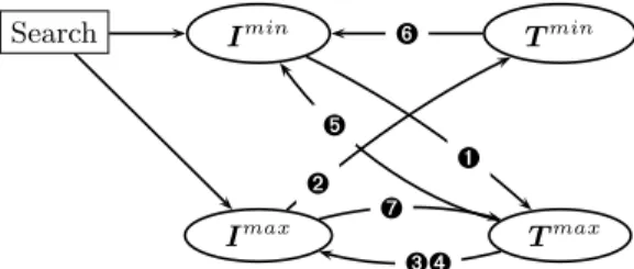
Search Imin Tmin Imax Tmax ➊ ➌➍ ➋ ➎ ➐ ➏
Fig. 1.Propagators for itemset mining as functions between bounds of variables; the search is assumed to branch over items.
algorithms likeEclatare more flexible; the choice of representation for sets is often left open. Considering supported constraints, the originalEclatalgorithm deals mainly with one type of constraint: the minimum frequency constraint. For other types of constraints, such as closedness constraints, the algorithm needs to be (and has been) extended. Gecode on the other hand supports many different constraints out-of-the-box, and imposes no restriction on which ones to use, or how to combine them.
To compare propagator activation in Eclat and Gecode, let us consider when the change of a variable is propagated. Figure 1 visualizes the propagation that is necessary for the constraints presented in Table 1. In the case of frequent itemset mining, only propagations➊and➌are strictly needed; propagation➋is useless as the lower-bound of the transaction variables (representing transactions that are certainly covered) is never used later on. Indeed Eclatonly performs propagation ➊ and ➌. However, Gecode activates propagators more often (to no possible beneficial effect in itemset mining). The reason is that in Gecode a propagator is activated whenever a variable’s domain is changed, independent of whether the upper-bound or lower-bound changed (similar to AC-3). Hence, if an item’s domain changes after frequency propagation, the coverage propagator will be triggered again already due to the presence of constraint➊1
.
Conclusion Overall, we can observe that the search procedures are similar at a high level, but that the constraint programming system faces significant overhead in data representation, data maintenance, and constraint activation.
4
An Integrated Approach
We propose an integrated approach that builds on the generality of CP, but aims to avoid the overhead of existing systems. Our algorithm implements the basic constraint search algorithm depicted in Algorithm 2, augmented with the following features: (1) a boolean vector as basic variable type; (2) support for multiple data representations; (3) a general matrix constraint that encompasses itemset mining constraints; (4) an auxiliary store in which facts are shared; (5) efficient propagators for matrix constraints. To the best of our knowledge, there
1 If we would enable propagation➋, the domain ofT may change; this would lead to
is currently no CP system that implements these features. In particular, our use of an auxiliary store that all constraints can access is uncommon in existing CP systems and mainly motivated by our itemset mining requirements.
Boolean vectors Our first choice is to use boolean vectors as basic variable types; such a vector can be interpreted as a subset of a finite set of elements, where the ith bit indicates if elementiis part of the set. Constraints will be posted on the set of itemsIand the set of transactionsT as a whole. We put no restriction on whether to implement the boolean vectors in a sparse or dense representation. The domain of a boolean vectorB is represented by its bounds in two boolean vectors,Bmin andBmax, as in [6]. We split a domain on one boolean.
Data representation When posting constraints, we support multiple matrix rep-resentations, such as vertical, horizontal, positive and negative representations. Constraints will operate on all representations, but more efficient propagators will be provided for some. Note that certain matrices can be seen as views on other matrices: for instance,DT is ahorizontal view on averticallyrepresented matrix D. Doing this avoids that different constraints need to maintain their own representations of the data, and hence reduces the amount of redundancy. General matrix constraint We now reformulate the reified summation constraint of Equation (8) on boolean vectors. The general form of the reified matrix con-straint is the following:
X≥11≥2θ(A ·Y); (9)
both the first≥1 and second≥2can be replaced by a≤;X andY are boolean column vectors;Ais a matrix;·denotes the traditional matrix product; 1≥θ is
anindicator functionwhich is applied element-wise to vectors: in this case, if the ith component ofA ·Y exceeds thresholdθ, theith component of the result is 1; otherwise it is 0. In comparing two vectorsX1≥X2it is required that every component of X1 is not lower than the corresponding component ofY2.
For instance, the frequency constraint can now be formalized as follows: I≤1≥θ(DT·T), (10)
which expresses that only if the vector product of the transaction vectorT with column vector iof the data exceeds thresholdθ, theith component of vectorI can be 1.
We can reformulate many itemset mining problems using this notation, as shown in Table 1. In this notation we assume that (x− A) yields a matrixA′in
whichA′
ij=x− Aij; furthermore,C represents a diagonal matrix in which the
costs of items are on the diagonal.
As with any CP system, other constraints and even other variable types can be added; for the typical itemset mining settings discussed in this paper no other constraints are needed.
Propagation framework A propagator for the general matrix constraint above can be thought of as a function taking boolean vectors (representing bounds) as input, and producing a boolean vector (representing another bound) as output. This is similar to how binary constraints are dealt with in the AC-5 propagation
strategy. For example, a propagator for the frequency constraint in Equation 10 is essentially a function that derives Imax from Tmax. Figure 1 lists all these relationships for the constraints in Table 1. In our system, we activate the propa-gator of a constraint only if the bound(s) it takes as input have changed, avoiding useless propagation calls.
Auxiliary store The main idea is to store a set of simple, redundant constraints that are known to hold given the constraints and the current variable assign-ments. These constraints are of the formX ⊆ Ai, where⊆may be replaced by
other set operators, X is a vector variable in the constraint program, and Ai
may also be a column in the data. Propagators may insert such constraints in the store and may use them later on to avoid data access and the subsequent computation. Note that the worst case size of this store isO(m+n).
Efficient Propagators The general propagator for one particular choice for the inequality directions in the matrix constraint,X ≤1≥θ(A ·Y),is the following:
Xmax←min(Xmax,1≥θ(A ·Ymax)), (11)
where we presumeAonly contains non-negative entries. This propagator takes as input vector Ymax and computes Xmax as output, possibly exploiting the
value Xmax currently has. Upon completion of the propagator, it should be
checked ifXmin≤Xmax; otherwise a contradiction is found and the search will
backtrack.
We provide the specialized propagators of the coverage and frequency con-straint on a vertical representation of the data below. We lack the space to provide details for other propagators.
Coverage: The coverage constraint is T ≤1≤0(A ·I),where A = 1− D, i.e. a binary matrix represented vertically in a negative representation whereDis the positive representation. The propagator should evaluateTmax←min(Tmax,1
≤0(A·
Imin)).Taking inspiration from itemset mining (Equation (5)), we can also
eval-uate this propagator as follows:
Tmax←Tmax∩( \
i∈Imin
DT
i). (12)
Observe that the propagator uses the vertical matrix representation DT di-rectly, without needing to compute the negative matrixA. The propagator skips columns which are not currently included in the itemset (i∈Imin). After having
executed this propagator, we know for a number of itemsi∈ IthatT ⊆ DT
i.We
will store this knowledge in the auxiliary constraint store to avoid recomputing it. The propagator is given in Algorithm 3.
Frequency: The minimum frequency constraint is I ≤ 1≥θ(A ·T), where A is
here a binary matrix horizontally represented; henceA=DT, for the vertically represented matrixD. The propagator should evaluate:
Algorithm 3PropCoverage(P,D) 1: LetIminpoint to input ofP inD
2: LetTmaxpoint to output ofPinD
3: for alli∈Imindo 4: if (Tmax⊆ DT i)6∈storethen 5: Tmax:= Tmax∩ DT i 6: Add (Tmax⊆ DT i) to store 7: end if 8: end for Algorithm 4PropFrequency(P,D) 1: LetTmaxpoint to input ofP in D
2: LetImaxpoint to output ofP inD 3: F :=|Tmax|
4: for alli∈Imaxdo 5: if (Tmax⊆ DT i)6∈storethen 6: F′:=|DT iT max | 7: ifF′< θthenImax i := 0 8: ifF′=F then 9: Add (Tmax⊆ DT i) to store 10: end if 11: end for
We can evaluate this constraint by computing for everyi∈Imaxthe size of the
vector product|DT
i ·Tmax|. If this number is lower thanθ, we can setIimax= 0.
We can speed up this computation using the auxiliary constraint store. If for an itemiwe know thatTmax⊆ DT
i, then|DTi ·Tmax|=|Tmax|so we only have
to compute|Tmax| ≥θ. The propagator can use the auxiliary store for this; see
Algorithm 4. This is the same information that the coverage constraint uses; hence it can happen at some point during the search that the propagators do not need to access the data any longer. Storing and maintaining the additional information in the auxiliary constraint store will require additional O(m+n) time and space for each itemset (as we need to store an additional transaction set or itemset for each itemset); the potential gain in performance in the frequency propagators isO(mn), as we can potentially avoid having to consider all elements of the data again.
5
Analysis
In this section we study the complexity of our constraint programming system on itemset mining tasks. Assuming that propagators are evaluated in polynomial space, the space complexity of the approach is polynomial, as the search proceeds depth-first and no information is passed from one branch of the search tree to another. In general, polynomial time complexity is not to be expected since CP systems can be used to solve NP complete problems.
For certain tasks, however, we can provepolynomial delaycomplexity, i.e. be-fore and after each solution is printed, the computation time is polynomial in the size of the input. In particular, the CP-based approach provides an alternative to the recent theory of accessible set systems [2], which was used to prove that certain closed itemset mining problems can be solved with polynomial delay.
Consider propagation of constraints in our system, if k is the sum of the lengths of the boolean vector variables in the constraint program for a problem, a fixed point will be reached inO(k) iterations, as this is the maximum number of bits that may change in all iterations of a propagation phase together. If each
propagator can be evaluated in polynomial time, then a call to Propagate(D) will execute in polynomial time. Using this we can prove the following.
Theorem 1. If all propagators and the variable selection functionf can be eval-uated in time polynomial in the input, and each failing node in the search tree has a non-failing sibling, solutions to the constraint program will be listed with polynomial delay by Algorithm 2.
Proof. Essentially we need to show that the number of failing leaves between two successive non-failing leaves of the search tree is polynomial in the size of the input. Assume we have an internal node, then given our assumption, independent of the order in which we consider its children, we will reach a succeeding leaf after considering O(k) nodes in the depth-first search. Consider the successive non-failing leaf, we will need at mostO(k) steps to reach the ancestor for which we need to consider the next child. From the ancestor we will reach the non-failing leaf after consideringO(k) nodes.
From this theorem follows that frequent and frequent closed itemsets can be listed with polynomial delay: considering a model without the useless propagator ➋(see Section 3), in a node’s child either an item is set to 1 or to 0, changing either Imin or Imax. When Imax changes, no propagation will happen, which
provides us one branch that does not fail, as required by the theorem.
The same procedure can also be used for more complex itemset mining prob-lems. We illustrate this here for a simple graph mining problem introduced in [3], which illustrates at the same time how our approach can be extended to other mining problems. In addition to a traditional itemset database, in this problem setting a graphG is given in which items constitute nodes and edges connect nodes. An itemset I satisfies constraint connected(I) if the subgraph induced in G by the nodes in I is connected. An itemset (I, T) satisfies con-straint connectedClosed(I, T) iff I corresponds to a complete connected com-ponent in the (possibly unconnected) subgraph induced in G by the nodes in ψ(T) =∩t∈TDt. We can solve this problem by adding the following elements in
the CP system:
– the coverage and frequency constraint as in standard itemset mining;
– a propagator forconnected(I), which takes Imax as input andImax as
out-put; given one arbitrary variable for which Imin
i = 1, it determines the
connected component induced by Imax that i is included in, and changes
the domainIimax = 0 for all items i not in this component. It fails if this
means that for somei′:Iimin′ > I
max i′ ;
– a propagator forconnectedClosed(I, T), which for a given setTmaxcalculates ψ(Tmax), and setsIimin= 1 for all items in the component the current items
inImin are included in, possibly leading to a failure;
– a variable selection functionf which as next item to split on selects an item which is connected inGto an item for whichImin
i = 1.
The effect of the variable selection function is that the propagator forconnected(I) will never fail in practice. Given the absence of another propagator depending onImax, the requirements for the theorem are fulfilled.
6
Experiments
In our experiments we aim to determine how much our specialized framework can contribute to reducing the performance gap between CP systems and item-set miners. As CP is particularly of interest when dealing with many different types of constraints, our main interest is achieving competitive behavior across multiple tasks.
Fairly comparing itemset miners is however a daunting task, as witnessed by the large number of results presented in the FIMI competition [9]. We report a limited number of settings here and refer to our website for more information, including the source code of our system2
.
We choose to restrict our comparison to the problems of frequent, closed and maximal itemset mining, as well as frequent itemset mining under a minimum size constraint. The reason is that there are a relatively large number of systems supporting all these tasks, some of which were initially developed for the FIMI competition, but have since been extended to deal with additional constraints. This makes these systems a good test case for how easily and efficiently special-ized algorithms can be extended to deal with additional constraints. In partic-ular, we used these systems: DMCP: our new constraint programming system, in which we always used a dense representation of sets and used a static or-der of items; FIMCP: our implementation based on Gecode [8]; PATTERNIST: the engine underneath the ConQueSt constraint-based itemset mining sys-tem [4]; LCM: an algorithm from the FIMI competition, in two versions [15]; ECLAT, ECLAT NOR, FPGrowth and APRIORI, as implemented by Borgelt [5]. ECLAT checks maximality of an itemset by searching for related itemsets in a repository of already determined maximal itemsets; ECLAT NOR checks the maximality of an itemset in the data. Unless mentioned otherwise, the algo-rithms were run with default parameters; output was requested, but written to /dev/null. The algorithms were run on machines with Intel Q9550 processors and 8GB of RAM. Experiments were timed out after 1800s.
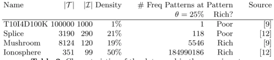
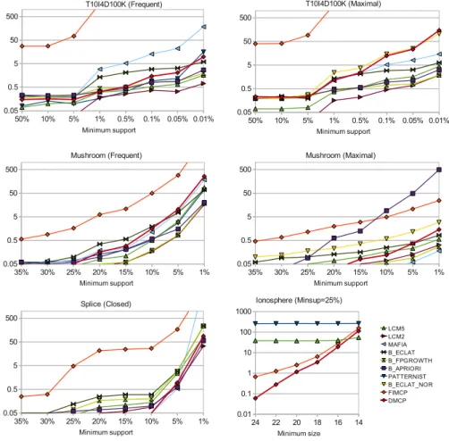
Characteristics of the data sets are given in Table 2. We can make a distinc-tion betweenpattern-poor datasets in which the number of frequent itemsets is small (the number of frequent itemsets at a minimum support of 25% is smaller than the number of items in the database; here post-processing a pre-computed set of patterns is an option for most constraints), andpattern-richdatasets for which the number of frequent itemsets is large. We are interested in the behavior of our system in both settings. All results are given in Figure 2.
Pattern-rich Data. On data with a large number of frequent itemsets, the use of constraints is necessary to make the mining feasible and useful. Compared to frequent itemset mining, maximal frequent itemset mining imposes more con-straints; hence we would expect constraint programming to be beneficial in this setting. Indeed, on the Mushroom data we can observe that DMCP outperforms approaches such as B APRIORI and B ECLAT NOR, which in this case are
Name |T | |I|Density # Freq Patterns at Pattern Source θ= 25% Rich? T10I4D100K 100000 1000 1% 1 Poor [9] Splice 3190 290 21% 118 Poor [12] Mushroom 8124 120 19% 5546 Rich [9] Ionosphere 351 99 50% 184990186 Rich [12]
Table 2.Characteristics of the data used in the experiments
filtering frequent itemsets3
. The CP-based FIMCP does not sufficiently profit from the propagation to overcome its redundant data representation.
Investigating the use of constraints further, we apply a number of mini-mum size constraints on the Ionosphere data. A minimini-mum size constraint is a common test case in constraint-based itemset mining, as it has a monotonicity property which is opposite to that of the frequency constraint. Some itemset mining implementations, such as LCM, have added this constraint as an op-tion to their systems. The results show that on this type of data, LCM and the PATTERNIST system, which was designed for constraint-based mining, are (almost) not affected by this constraint; the CP based approaches, on the other hand, can effectively prune the search space as the constraint becomes more restrictive, where DMCP is again superior to FIMCP.
Pattern-poor Data. We illustrate the behavior of the systems on pattern-poor data using the T10I4D100K dataset for frequent and maximal itemset mining, and using Splice for closed itemset mining. In all cases, FIMCP suffers from its redundant representation of the sparse data. For most systems, the run time is not affected by the maximality constraint. The reason is that the number of maximal frequent itemsets is very similar to that of the total number of frequent itemsets. In particular in systems such as B ECLAT and B FPGROWTH, which use a repository, the maximality check gives minimal overhead. If we disable the repository (B ECLAT NOR), Eclat’s performance is very similar to that of the DMCP system, as both systems are essentially filtering itemsets by checking maximality in the data. Similar behavior is observed for the splice data, where the difference between closed and non-closed itemsets is small. In all figures it is clear that our system operates in the same ballpark as other itemset mining systems.
7
Conclusions
In this paper we studied the differences in performance between general CP solvers and specialized mining algorithms. We focused our investigation on the representation of the data and the activation of propagators. This provided in-sights allowing us to create a new algorithm based on the ideas of AC-5 con-straint propagation; it uses boolean vectors as basic type, supports general ma-trix constraints, enables multiple data representations and uses an auxiliary store
3 The difference between B APRIORI and B ECLAT NOR is mainly caused byperfect extension pruning[5], which we did not disable.
Fig. 2.Run times in seconds of several algorithms; see the main text for a discussion.
inspired by the efficient constraint evaluations of itemset mining algorithms. Additionally, we demonstrated how the framework can be used for complexity analysis of mining tasks and illustrated this on a problem in graph mining. We showed experimentally that our system overcomes most performance differences. Many questions have still been left unanswered. At the moment, we imple-mented the optimized propagators in a new CP system which does not support the wide range of constraints general systems such as Gecode do. Whether it is possible to include the same optimizations in Gecode is an open question. An-other question is which An-other itemset mining strategies can be incorporated in a general constraint programming setting. An essential component of our current approach is that constraints express a relationship between items and transac-tions. However, other itemset mining systems, of which FP-Growth [11] is the most well-known example, represent the data more compactly by merging identi-cal transactions during the search; as our current approach builds on transaction identifiers, this approach faces problems.
Finally, the use and possible extension of constraint programming for dealing with other data mining problems than itemset mining is the largest challenge we are currently working on.
Acknowledgements. This work was supported by a Postdoc and a project grant from the Research Foundation—Flanders, project “Principles of Patternset Mining”, as well as a grant from the Institute for the Promotion and Innovation through Science and Technology in Flanders (IWT-Vlaanderen).
References
1. R. Agrawal, H. Mannila, R. Srikant, H. Toivonen, and A. I. Verkamo. Fast discovery of association rules. InAdvances in Knowledge Discovery and Data Mining, pages 307–328. AAAI Press, 1996.
2. H. Arimura and T. Uno. Polynomial-delay and polynomial-space algorithms for mining closed sequences, graphs, and pictures in accessible set systems. In SDM, pages 1087–1098. SIAM, 2009.
3. M. Boley, T. Horv´ath, A. Poign´e, and S. Wrobel. Efficient closed pattern mining in strongly accessible set systems. InPKDD, pages 382–389, 2007.
4. F. Bonchi, F. Giannotti, C. Lucchese, S. Orlando, R. Perego, and R. Trasarti. A constraint-based querying system for exploratory pattern discovery. Inf. Syst., 34(1):3–27, 2009.
5. C. Borgelt. Efficient implementations of Apriori and Eclat. InWorkshop of Fre-quent Item Set Mining Implementations (FIMI), 2003.
6. C. Bucila, J. Gehrke, D. Kifer, and W. M. White. Dualminer: A dual-pruning algorithm for itemsets with constraints. Data Min. Knowl. Discov., 7(3):241–272, 2003.
7. D. Burdick, M. Calimlim, J. Flannick, J. Gehrke, and T. Yiu. MAFIA: A maximal frequent itemset algorithm. IEEE TKDE, 17(11):1490–1504, 2005.
8. L. De Raedt, T. Guns, and S. Nijssen. Constraint programming for itemset mining. InKDD, pages 204–212, 2008.
9. B. Goethals and M. J. Zaki. Advances in frequent itemset mining implementations: report on FIMI’03. InSIGKDD Explorations, volume 6, pages 109–117, 2004. 10. J. Han, L. V. S. Lakshmanan, and R. T. Ng. Constraint-based multidimensional
data mining. IEEE Computer, 32(8):46–50, 1999.
11. J. Han, J. Pei, and Y. Yin. Mining frequent patterns without candidate generation. InProceedings of the ACM SIGMOD International Conference on Management of Data, pages 1–12, 2000.
12. S. Nijssen, T. Guns, and L. De Raedt. Correlated itemset mining in ROC space: a constraint programming approach. InKDD, pages 647–656, 2009.
13. F. Rossi, P. van Beek, and T. Walsh.Handbook of Constraint Programming (Foun-dations of Artificial Intelligence). Elsevier Science Inc., 2006.
14. C. Schulte and P. J. Stuckey. Efficient constraint propagation engines.Transactions on Programming Languages and Systems, 31(1), 2008.
15. T. Uno, M. Kiyomi, and H. Arimura. LCM ver.3: collaboration of array, bitmap and prefix tree for frequent itemset mining. InOSDM ’05: Proceedings of the 1st international workshop on open source data mining, pages 77–86, 2005.
16. M. J. Zaki, S. Parthasarathy, M. Ogihara, and W. Li. New algorithms for fast discovery of association rules. InKDD, pages 283–286, 1997.