Parametric estimation of complex mixed models based
on meta-model approach
Pierre Barbillon, C´
elia Barth´
el´
emy, Adeline Samson
To cite this version:
Pierre Barbillon, C´
elia Barth´
el´
emy, Adeline Samson. Parametric estimation of complex mixed
models based on meta-model approach. 2015.
<
hal-01162351
>
HAL Id: hal-01162351
https://hal.archives-ouvertes.fr/hal-01162351
Submitted on 10 Jun 2015
HAL
is a multi-disciplinary open access
archive for the deposit and dissemination of
sci-entific research documents, whether they are
pub-lished or not.
The documents may come from
teaching and research institutions in France or
abroad, or from public or private research centers.
L’archive ouverte pluridisciplinaire
HAL
, est
destin´
ee au d´
epˆ
ot et `
a la diffusion de documents
scientifiques de niveau recherche, publi´
es ou non,
´
emanant des ´
etablissements d’enseignement et de
recherche fran¸cais ou ´
etrangers, des laboratoires
publics ou priv´
es.
Parametric estimation of complex mixed models
based on meta-model approach
Pierre Barbillon
1,2, Célia Barthélémy
3, and Adeline Samson
4,5 1AgroParisTech / UMR INRA MIA, F-75005 Paris
2
INRA, UMR 518, F-75005 Paris
3INRIA Saclay, Popix team, Orsay
4
Univ. Grenoble Alpes, LJK, F-38000 Grenoble, France
4CNRS, LJK, F-38000 Grenoble, France
June 10, 2015
Abstract
Complex biological processes are usually experimented along time among a collection of individuals. Longitudinal data are then available and the statisti-cal challenge is to better understand the underlying biologistatisti-cal mechanisms. The standard statistical approach is mixed-effects model, with regression functions that are now highly-developed to describe precisely the biological processes (solu-tions of multi-dimensional ordinary differential equa(solu-tions or of partial differential equation). When there is no analytical solution, a classical estimation approach relies on the coupling of a stochastic version of the EM algorithm (SAEM) with a MCMC algorithm. This procedure needs many evaluations of the regression function which is clearly prohibitive when a time-consuming solver is used for computing it. In this work a meta-model relying on a Gaussian process emulator is proposed to replace this regression function. The new source of uncertainty due to this approximation can be incorporated in the model which leads to what is called a mixed meta-model. A control on the distance between the maximum likelihood estimates in this mixed meta-model and the maximum likelihood esti-mates obtained with the exact mixed model is guaranteed. Eventually, numerical simulations are performed to illustrate the efficiency of this approach.
Keywords: Mixed models, Stochastic EM algorithm, MCMC methods, Gaussian Process emulator.
1
Introduction
Mixed-effects model methodology (Pinheiro and Bates, 2000) allows to discriminate between inter- and intra-subjects variabilities which is essential when dealing with lon-gitudinal data. Statistical methods for mixed models are now well established (see
references below) but can be time consuming depending on the complexity of the re-gression functions. Indeed sophisticated mathematical models have been developed to describe precisely biological processes: multi-dimensional ordinary differential equations (ODE) (see Wu et al., 2005; Guedj et al., 2007; Lavielle et al., 2011; Ribba et al., 2012, for modeling viral load decrease in HIV patients or tumor growth) or partial differ-ential equation (PDE) (see Grenier et al., 2014; Chatterjee et al., 2012, for modeling tumor growth or HVC viral kinetic). These mathematical models have no analytical solution and only an approximate solution can be obtained with computationally in-tensive numerical methods. This induces a huge increase of the computation cost of the estimation method (up to 23 days according to Grenier et al., 2014). Therefore, there is a crucial need to develop new statistical approaches to reduce the computation time. The significant computation time of mixed models estimation methods is due to their iterative settings, compulsory to sidestep the intractability of the likelihood. This is true for methods based on linearisation (Pinheiro and Bates, 2000) or likelihood numerical approximation (Davidian and Giltinan, 1995; Wolfinger, 1993) and this is crucial for EM-type methods such as stochastic EM algorithms (Wei and Tanner, 1990; Kuhn and Lavielle, 2005).
Our objective is to propose a way of reducing the computation time of the SAEM-MCMC algorithm (Kuhn and Lavielle, 2005) for complex mixed models, together with a theoretical study of the resulting estimator. When the regression function is not analytically available (and we call it also computer model in the rest of the paper), extensions of SAEM have already been proposed. Donnet and Samson (2007) deal with the case of an ODE mixed model, approximating the solution with a numerical scheme and studying the influence of this scheme to the properties of the approximate maximum likelihood estimator. But this approach remains time consuming when the ODE is multi-dimensional. For a PDE mixed model, Grenier et al. (2014) propose to approximate the PDE with a numerical scheme on a predefined grid, and then to interpolate the solution of the PDE linearly between two points of the grid. This linear approximation allows substantially reducing the computation time from 23 days to around 30 minutes, but may lead to biased estimates depending on the non linearity of the model.
The keystone of providing an efficient estimation method with good statistical proper-ties is the choice of the procedure approximating the regression function. More accurate surrogates of computer model than linear approximation rely on Gaussian process em-ulation which consists of modeling the computer model as the realization of a Gaussian process (Sacks et al., 1989; Santner et al., 2003; Fang et al., 2005). This technique is also known as Kriging. A cheap approximation of the model, the emulator, is obtained by conditioning the Gaussian process on some evaluations of the model corresponding to inputs of a well-chosen design of numerical experiments. This stochastic modeling of the computer model provides also a measure of uncertainty on the precision of the approxi-mation as a supplementary variance-covariance function which can be integrated in the mixed model. This approach has been already coupled with a Stochastic EM algorithm (Barbillon et al., 2011) or with a Bayesian procedure (Fu et al., 2014) in regression mod-els without random effects. In this paper, we propose to couple the SAEM algorithm with this Gaussian process emulator, incorporating this new source of uncertainty due
to the approximation. Thus, providing a confidence interval of the unknown parame-ters takes into account the error induced by the approximation. We will refer to this approach as the complete mixed meta-model. However, the supplementary variance-covariance function in the model induces a loss of independence of the observations obtained from the different subjects which increases the computational burdensome of the MCMC scheme. That is why we also propose two simplified versions: the first one (called intermediate) by considering a diagonal variance-covariance function of the approximation error; the second one (called simple) by only using the approximation of the computer model and not incorporating the variance-covariance function. These two last versions allow to assume the independence between the subjects, and to reduce significantly the computational cost.
The Gaussian process emulator can also be interpreted as an approximation of the com-puter model by kernel interpolation with radial basis function as in Schaback (1995, 2007). In this framework, a point-wise control on the error of approximation is pro-vided. Hence, we are able to guarantee a control on the distance between the maximum likelihood estimates in the approximate mixed meta-models and the maximum likeli-hood estimates obtained with the exact computer model. This control is decreasing to zero as a function of the space-fillingness of the design of numerical experiments. The paper is organized as follows. Section 2 introduces the standard non-linear mixed model and Section 3 recalls the principles and the main results of the Gaussian process emulation. Section 4 introduces three mixed models approximated by Gaussian process emulator. In Section 5, three versions of the SAEM algorithm coupled to a Gaussian process emulator are proposed. Theoretical results are given in Section 6. A simulation study illustrates these results (Section 7). Section 8 concludes the paper with some extensions. Proofs are gathered in Appendix.
2
Mixed model and notations
Let us define yi = t(yi1, . . . , yini) where yij ∈ R
p is the response for individual i at
time tij, i = 1, . . . , N, j = 1, . . . , ni, and let y = (y1, . . . ,yN) be the vector of all
observations, of size ntot = PNi=1ni. We assume that the individual vectors yi are
described by a non-linear mixed model, defined as follows, forj= 1, . . . , ni:
yij = f(tij, ψi) +σεεij, εij∼iid N(0,1), (1)
ψi ∼iid N(µ,Ω),
where f(·,·) : R×Rd → Rp is the regression function, ψi is a d-vector of individual
parameters. The εi = (εi1, . . . , εini)
t represents the Gaussian centered residual error,
independent of ψi. The individual parameterψi are assumed to be random, Gaussian
with expectation µ and d×dcovariance matrix Ω. Note that the individual vectors
(yi)i are independent and identically distributed.
The quantities we want to estimate from the observations y are the population pa-rametersθ= (µ,Ω, σ2
ε). In the following, we restrict to the case of scalar observations
(p= 1) to ease the reading, but the extension to a multidimensional observation with p >1is straightforward.
We want to estimateθby maximum likelihood. The likelihood of model (1) is: p(y, θ) = Z p(y,ψ;θ)dψ= N Y i=1 Z p(yi|ψi;θ)p(ψi;θ)dψi = N Y i=1 Z ( 1 (2πσ2 ε)ni/2 ×exp −1 2 t(y i−f(ti, ψi))(σε2Ini) −1(y i−f(ti, ψi)) × 1 (2π)d/2|Ω|1/2exp −1 2 t(ψ i−µ)Ω−1(ψi−µ) dψi ) (2) whereti= (ti1, . . . , tini)and
f(ti, ψi) = t(f(ti1, ψi), . . . , f(tini, ψi)). When f is non linear with respect toψ, the
maximum likelihood estimator has no closed form. Any estimation method adapted to non-linear mixed models would require a very large number of evaluations of f, which could be time consuming when the structural function f is a computer model. Therefore, there is a real need to consider approximations of the function f that are simple to evaluate at any point (t, ψ). For that purpose, we introduce the framework of meta-model in the next section.
3
Meta-model
We start with the point of view of conditioned Gaussian process emulation which has the nice feature of incorporating as a variance-covariance function the additional source of uncertainty due to the approximation. This will naturally lead to a mixed meta-model on which the SAEM-MCMC can be performed. We also link this framework to the kernel interpolation framework since we need the deterministic point-wise control on the approximation to obtain the control between the maximum likelihood estimates corresponding to the exact model and to its approximation.
3.1
Conditioned Gaussian process
In this framework, the function f is interpreted as a realization of a Gaussian Process. Let us denoteFλ a Gaussian process defined, for anyx= (t, ψ), as
Fλ(x) = L
X
j=1
βjhj(x) +ζ(x) = tH(x)β+ζ(x), (3)
whereh1, . . . , hLare regression functions,H = (h1, . . . , hL),β= (β1, . . . , βL)is a vector
of parameters,ζis a centered Gaussian process with covariance function Cov(ζ(x), ζ(x′)) =σ2Kφ(x, x′),
where Kφ is a correlation function depending on some parametersφ andλ= (β, σ, φ)
is the vector of all unknown parameters. For instance, the so-called Gaussian kernel is defined by Kφ(x, x′) = exp(−φkx−x′k2). The regression functions h1, . . . , h
usually linear functions or low degree polynomials. The kernelKφhas to be chosen with
respect to the assumed regularity of the functionf. Similarly, the regression functions H have to be chosen with respect to the supposed trend in the function f if some insights on the function are available. See Koehler and Owen (1996); Fang et al. (2005) for detailed discussions on the choice of the regression functions and kernels.
We assume that we are able, in a pre-computation step, to evaluate precisely the func-tionf nD times for a given design of numerical experiments,D={x1, . . . xnD}. These "exact" evaluations are denoted z1 =f(x1), . . . , zn = f(xnD). The (zk) are different from the (yij)considered in model (1) which are noisy observations of f in some
un-known points x= (t,ψ). The design of experiments D is usually chosen with respect to a space-filling criterion (Fang et al., 2005) in a bounded domain where the points
(tij, ψi)i,j are assumed to be. For a given kernelK, and a given vectorH of regression
functions, the vector of parameters λhas to be estimated. Usually,λ is estimated by maximizing the log-likelihoodℓF of the Gaussian processF (3):
ℓF(λ;zD) = − 1 2log((2πσ 2)nD| ΣφDD|) (4) −1 2 t(z D−HDβ)(σ2ΣφDD)−1(zD−HDβ), where(ΣφDD)1≤k,j≤nD = (K φ(x
k, xj)),(HD)1≤k≤nD,1≤j≤L=hj(xk). The Matlab tool-box DACE (Lophaven et al., 2002) provides an optimization algorithm to estimate directly λ. We denote byˆλ= (ˆβ,σ,ˆ φˆ)the estimates. The Gaussian process is chosen to beF =Fˆλ. It corresponds to a plug-in approach since from now, these parameters are considered as known.
Thenfis not directly approximated byF, but rather by the conditional process denoted FD, defined as the processF conditionally toF(x1) =z1, . . . , F(x
nD) =znD, in short
ZD=zD. The processFDis still a Gaussian process, defined by its mean and covariance
functions, which can be exactly computed. Let us introduce the partial functions, for any x ∈ Rd+1, Kxφ : Rd+1 → R defined by Kxφ(x′) = Kφ(x, x′) for any x′ and the
vector ΣφxDˆ =Kφˆ x(xk)
1≤k≤nD
. Then, the meanmD(x) and covarianceCD(x, x′) of
the processFDare defined, for all x, x′ as
mD(x) =H(x)tβˆ +tΣ ˆ φ xD(Σ ˆ φ DD)−1(zD−HDβˆ), (5) CD(x, x′) = ˆσ2(K ˆ φ x(x′)− tΣ ˆ φ xD(Σ ˆ φ DD) −1Σφˆ x′D). (6)
The mean function mD provides an approximation of the function f for any x and
the variance function x 7→ CD(x, x) measures the confidence in the accuracy of this
approximation. The plug-in approach for λ = (β, σ2, φ) may lead to underestimate the uncertainty on the quality of the approximation which is showed to be asymptot-ically negligible (Prasad and Rao, 1990). It can be used only for the parameter of the correlation kernel φ. In this case, when the process is not conditioned on (ˆβ,σˆ), the conditioned process is a Student T-process with still closed-form location and scale (Santner et al., 2003). However, we prefer the complete plug-in approach to deal with a Gaussian distribution which is easier to incorporate in the mixed model.
3.2
Kernel interpolation
We can interpret the previous meta-model approximation as a kernel interpolation. In-deed, a Reproducing Kernel Hilbert Space (RKHS) can be associated toKφas soon as
the kernelKφ is positive definite. Then the partial functionsKφ
x defined in Section 3.1
span a pre-Hilbert space with inner product< Kφ x, K
φ
x′ >=Kφ(x, x′). Aronszajn’s
the-orem states that there exists a unique completionHKof this space with the reproducing
property:
∀v∈ HK, x∈Rd+1, v(x) =< v, Kxφ> .
The space HK is the RKHS associated to kernel K. Then, we focus on the function
g(x) =f(x)− tH(x)ˆβ, whereβˆ is estimated as before. Note that this function can be
seen as the residuals of the linear model (3) of the random variablesZ1, . . . , ZnD on the designD={x1, . . . xnD}:
Zi=f(xi) = tH(xi)ˆβ+g(xi).
We consider the following problem of seeking for the function inHK which interpolates
g on points ofDwith a minimal norm:
minv∈HKkvkHK
g(xk) =v(xk), k= 1, . . . nD.
The solution to this problem is the orthogonal projection ofgon the subspace spanned by (Kx1, . . . , KxnD), denoted sK,D(g). If we assume that the function g =f −
tHβˆ
belongs toHK, thensK,D(g)is defined as
sK,D(g(x)) = tΣ ˆ φ xD(Σ ˆ φ DD) −1(z D−HDβˆ) (7) = tu(x)(z D−HDβˆ) = nD X k=1 uk(x)g(xk), with tu(x) = tΣφˆ xD(Σ ˆ φ
DD)−1 (same notations as in Section 3.1). This provides an
approximation off which is the same than the function mD (5). The approximation
mDbelongs to the RKHS assuming that the regression functionsHbelong to the RKHS,
which is true for linear or low degree polynomial regressorsH.
The kernel interpolation framework yields to an upper bound on the point-wise error of this approximation using the reproducing property and a Cauchy-Schwarz inequality. For anyx, we have
|f(x)−mD(x)| = |g(x)−sK,D(g(x))| ≤ |< g, Kxφˆ− nD X k=1 uk(x)K ˆ φ xk >| ≤ kgkHK· kK ˆ φ x− nD X k=1 uk(x)K ˆ φ xkkHK =: kgkHKPD(x). (8)
The normkgkHK is unknown and depends onf. The normPD(x)does not depend on f (org) but on the design of experimentsD only. It holds that
PD(x) = (K ˆ φ(x, x)− tΣφˆ xD(Σ ˆ φ DD) −1Σφˆ xD) = 1 ˆ σ2CD(x, x).
Again, there exists a link with the Gaussian process framework: up to the parameter
ˆ
σ2, we obtain the variance function of the conditioned Gaussian process (6).
For some usual kernels, a uniform upper-bound onPD(x)is available as a function of
aD= sup x∈Xd+1
min
1≤k≤nD
kx−xkk
whereX is a bounded subspace ofR. The value ofaDis related to the coverage of the
space X by the design of experiments. A design of experiments which minimizes this quantity is said to be minimax (Johnson et al., 1990). The point-wise upper bound is given in the following Proposition (Schaback, 1995):
Proposition 1. Assume that the experimental design D is minimax in X. Let HK
denote the RKHS associated to the kernel K which is assumed to be derived from a
radial basis function as proposed in Wu and Schaback (1992). Assume that f lies in
HK. LetmD denote the kernel approximation of the function f obtained on the design
D. Then the point-wise error|f(x)−mD(x)| is uniformly upper-bounded inX by
|f(x)−mD(x)| ≤ kgkHKPD(x)≤ kgkHKGK(aD). where the function GK is defined onR+ and is such that lim
a→0+GK(a) = 0.
Furthermore, if the regressorsH ∈ HK, then there exists a constantC >0such that
|f(x)−mD(x)| ≤CkfkHKGK(aD).
For instance, when using a Gaussian kernelKφ(x, x′) =e−φkx−x′k2
, the functionGK is
GK(a) =Ce−δ/a 2
whereC andδare constants depending onφ.
4
Three mixed meta-models
The estimation of the population parameterθis performed on the meta-model approx-imation of the mixed model (1). For computational reasons, we introduce three mixed meta-models.
4.1
Complete mixed meta-model
Let us introduce the so-called complete mixed model that integrates the meta-model approximation. The regression functionf in (1) is approximated byFD(t, ψ) =
mD(t, ψ) +r(t, ψ):
yij = FD(tij, ψi) +σεεij, εij ∼iidN(0,1), (9)
ψi ∼iid N(µ,Ω),
FD(t, ψ) = mD(t, ψ) +r(t, ψ), with,
Whereas model (1) is homoscedastic (constant error variance), the mixed metamodel (9) is heteroscedastic. Let us emphasize thatthis is not a standard heteroscedastic error model. Indeed, we have:
yij|ψi∼ N(mD(tij, ψi),ΓD(tij, ψi))
with
ΓD(t, ψ) =σ2ε+CD(t, ψ;t, ψ),
but the (yij|ψi)j are not independent, as well as the individual vectors (yi)i. This is
due to the fact that the (r(tij, ψi))ij are realizations of the same Gaussian process.
This is a major difference with approximations that have already been proposed in the literature (Donnet and Samson, 2007; Grenier et al., 2014). Especially, this complicates the implementation of the MCMC scheme.
We propose to estimateθ as the maximum of the likelihood of model (9). We denote
mD(t,ψ) = (mD(tij, ψi))1≤i≤N,1≤j≤ni
the vector of the approximate mean, evaluated on(t,ψ) = (tij, ψi)1≤i≤N,1≤j≤ni. Simi-larly, we denote
CD(t,ψ) = (CD(tij, ψi;ti′j′, ψi′))1≤i,i′≤N,1≤j,j′≤ni. The likelihood of model (9) is then:
pD(y;θ) = Z ( p(ψ;θ) 1 (2π)ntot/2|σ2 εIntot+CD(t,ψ)|1/2 (10) exp −1 2 t(y−m D(t,ψ))(σε2Intot+CD(t,ψ)) −1(y−m D(t,ψ)) dψ ) . This likelihood is not explicit because functionmD(tij, ψi)is not linear inψi. As said
previously, this likelihood cannot be simplified as a product of individual likelihoods because the yi are not independent (the matrixCD(t,ψ)is a full matrix). The
corre-sponding estimation algorithm requires to invert thisntot×ntot-matrix at each iteration
(at least N×2dper iteration), which is highly computationally intensive. Therefore, we introduce an intermediate mixed meta-model by considering only the diagonal of
CD(t,ψ).
4.2
Intermediate mixed meta-model
In the intermediate mixed meta-model, the regression function f is approximated by mD(t, ψ)+¯r(t, ψ), wherer¯(t, ψ)has a diagonal covariance matrixΛi,ψi = diag(CD(ti, ψi)):
yij = mD(tij, ψi) + ¯r(tij, ψi) +σεεij, (11)
εij ∼iid N(0,1),
ψi ∼iid N(µ,Ω)
¯
The likelihood of model (11) is then: ¯ pD(y;θ) = N Y i=1 Z ( p(ψi;θ) 1 (2π)ni/2Qni j=1(σε2+CD((tij, ψi),(tij, ψi)))1/2 (12) exp −1 2 t(y i−mD(ti, ψi))(σε2Ini+ Λi,ψi) −1(y i−mD(ti, ψi)) dψi ) . This form of the likelihood is separable with respect to ψi and can be written as a
product over the individuals which are independent. The covariance matrixσ2
εIni+Λi,ψi is diagonal and can be easily inverted. This will substantially reduce the computation time of the estimation method. However the intermediate model is heteroscedastic, and σε might be more difficult to estimate than in the exact model. This is why we
introduce a simpler mixed meta-model.
4.3
Simple mixed meta-model
The simple mixed meta-model neglects the error of approximation of the computer model. The regression function is thenmD:
yij = mD(tij, ψi) +σεεij, εij∼iidN(0,1), (13)
ψi ∼iid N(µ,Ω).
The simple mixed meta-model (13) has similar properties than model (1): it is ho-moscedastic (constant error variance),the vectors(yi)i are independent and identically distributed, and for each individual i, conditionally to ψi, the (yij)j are independent.
The likelihood of model (13) is given by:
˜ pD(y;θ) = N Y i=1 Z ( p(ψi;θ) 1 (2πσ2 ε)ni/2 (14) exp −1 2 t(y i−mD(ti, ψi))(σ2εIni) −1(y i−mD(ti, ψi)) dψi ) , which has the same form than likelihood of model (1).
5
Population parameter estimation
Likelihoods of the mixed meta-models being not explicit, we resort to the family of EM algorithm to estimate the parameters θ, which is a classical approach for models with non-observed or incomplete data. We start with the SAEM algorithm for the exact mixed model and then for the three mixed meta-models.
5.1
Estimation for the exact mixed model
The objective is to maximize the likelihoodp(y;θ)of the exact mixed model (1). Let us briefly cover the EM principle (Dempster et al., 1977). The complete data of the
mixed model is(y,ψ). The EM algorithm maximizes theQ(θ|θ′) =E(L(y,ψ;θ)|y;θ′)
function in 2 steps, whereL(y,ψ;θ)is the log-likelihood of the complete data for the mixed model (1) andEis the expectation under the conditional distributionp(ψ|y;θ′).
At the k-th iteration, the E step is the evaluation of Qk(θ) = Q(θ|θb(k−1)), whereas
the M step updates θb(k−1) by maximizing Q
k(θ). For cases with a non analytic E
step, Delyon et al. (1999) introduce a stochastic version SAEM of the EM algorithm which evaluates the integral Qk(θ) by a stochastic approximation procedure. The E
step is then divided into a simulation step (S step) of the missing dataψ(k) under the conditional distribution p(ψ|y;bθ(k−1)) and a stochastic approximation step (SA step) of the conditional expectation, using(γk)k≥0 a sequence of positive numbers decreasing to 0:
Qk(θ) =Qk−1(θ) +γk(L(y,ψ(k);θ)−Qk−1(θ)).
In cases where the simulation of the non-observed vectorψcannot be directly performed, Kuhn and Lavielle (2005) propose to combine the SAEM algorithm with a Markov Chain Monte Carlo (MCMC) procedure. The idea is to simulate a Markov chainψ(k) by use of a Metropolis-Hastings (M-H) algorithm withp(ψ|y;θb(k−1))as the unique stationary distribution.
The complete data likelihoodL(y,ψ;θ)of the exact mixed model belongs to the regular curved exponential family:
p(y,ψ;θ) = exp{−ν(θ)+< S(ψ), λ(θ)>}
where < ·,· > denotes the scalar product, the minimal sufficient statistic S(y,ψ)
takes its values in an open subset S of Rm, νD and λ are functions of θ. Then the
SA step reduces to approximate EhS(y,ψ)|bθ(k−1)i at each iteration by the value s
k.
The sufficient statistics for the exact mixed model are classically S1(y,ψ) =PNi=1ψi,
S2(y,ψ) =PNi=1ψitψi and
S3(y,ψ) = PNi=1
Pni
j=1(yij −f(tij, ψi))2 (Samson et al., 2007). Then the M step is
explicit and easy to implement. The convergence of the SAEM-MCMC algorithm has been proved when the complete data likelihood belongs to the regular curved exponen-tial family and under additional assumptions (see Proposition 2). Thus the exponenexponen-tial family plays a crucial role to obtain an efficient algorithm.
5.2
Estimation for the simple mixed meta-model
The objective is to maximize the likelihood p˜D(y;θ)of the simple mixed meta-model
(13). In the following, all the quantities referring to this approximate likelihoodp˜D(y;θ)
are indexed by D with a tilde symbol. The corresponding complete data likelihood
˜
LD(y,ψ;θ) belongs to the regular curved exponential family with minimal sufficient
statisticsS˜D(y,ψ), which are the same as the exact mixed model. In that model, the
MCMC algorithm is easy to implement because of the independence of the observations of the individuals. More precisely, the SAEM-MCMC is described as follows.
Algorithm 1. (SAEM-MCMC algorithm for the simple mixed meta-model)
At iterationk, given the current values of the estimators µˆ(k−1),Ωˆ(k−1),σˆ2 (k−1)
Simulation step: For each individual iseparately and successively, update ψi(k)
with m iterations of an MCMC procedure with p˜D(ψi|yi;θb(k−1)) as stationary distribution:
Forl= 1. . . , m, given a current valueψil−1 for individual i:
– Simulate a candidate ψc
i with a proposal distributionqθb(k−1)(·|ψ l−1
i ).
– Meta-model step: Evaluate the meta-model
mD(tij, ψic)for allj = 1, . . . , ni.
– The candidate is accepted, ψl
i=ψic, with probability α˜i(ψic, ψil−1); otherwise the candidate is rejected, ψl
i =ψil−1 with probability1−α˜i(ψic, ψil−1), where
˜ αi(ψic, ψil−1) = min p˜ D(yi|ψic;bθ(k−1))p(ψci;θb(k−1)) ˜ pD(yi|ψil−1;bθ(k−1))p(ψ l−1 i ;θb(k−1)) qθb(k−1)(ψ l−1 i |ψci) qθb(k−1)(ψci|ψil−1) ,1 . Setψ(ik)=ψm i .
Stochastic Approximation step: update the sufficient statistics:
sk,1 = sk−1,1+γk N X i=1 ψ(ik)−sk−1,1 ! , sk,2 = sk−1,2+γk N X i=1 ψ(ik)tψi(k) −sk−1,2 ! , sk,3 = sk−1,3+γk N X i=1 ni X j=1 (yij−mD(tij, ψ(ik))) 2−s k−1,3 .
Maximisation step: update the population parameters
b µ(k) = sk,1 N , Ωb (k)= sk,2 N − sk,1tsk,1 N2 , σbε 2(k) = sk,3 ntot .
5.3
Estimation for the intermediate mixed meta-model
In the following, all the quantities referring to the approximate likelihood p¯D(y;θ) of
the intermediate mixed meta-model are indexed byDwith a bar symbol.
This model belongs to the exponential family when the Gaussian processr¯is considered in the hidden states. Then the complete data of the intermediate mixed meta-model are(y,ψ,¯r)where¯r= (¯r(tij, ψi))i=1,...,N,j=1,...,ni. The complete log-likelihood is thus:
¯
LD(y,ψ,¯r;θ) = log ¯pD(y|¯r,ψ;θ) + log ¯pD(¯r|ψ;θ) + logp(ψ;θ)
= cst−ntot 2 log(σ 2 ε)− 1 2 X ij (yij−mD(tij, ψi)−r¯(tij, ψi))2 σ2 ε −1 2 X i log(|Λi,ψi|)− 1 2 X i t¯rΛ−1 i,ψi¯r− N 2 log(|Ω|) −1 2 X i t(ψ i−µ)Ω−1(ψi−µ),
wherecstdenotes a constant term. The E-step is the computation of Q(θ|θb(k−1)) = E( ¯L D(y,ψ,¯r;θ)|y;θb(k−1)) = Z Z log ¯pD(y,¯r,ψ;θ)¯pD(¯r,ψ|y;θb(k−1))d¯rdψ = Z Z log ¯pD(y,¯r,ψ;θ)¯pD(¯r|y,ψ;θb(k−1))d¯r ¯ pD(ψ|y;θb(k−1))dψ.
The conditional distributionp¯D(¯ri|yi, ψi;bθ(k−1))is explicit, Gaussian, with mean and
covariance defined by ¯ m(r,ψk−i1) = ¯ Γ(r,ψk−i1)(yi−mD(ψi))/σc 2 ε (k−1) , ¯ Γ(r,ψk−i1) = (1/cσ 2 ε (k−1) + Λ−i,ψ1i) −1. Integrated with respect to¯rinsideQ(θ|bθ(k−1))yields to
Q(θ|θb(k−1)) = Z −ntot 2 log(σ 2 ε)− 1 2 X i kyi−mD(ti, ψi)−m¯(r,ψk−i1)k 2 σ2 ε − 1 2σ2 ε X i Tr(¯Γ(r,ψk−i1))− 1 2 X i log|Λi,ψi| −1 2 X i tm¯(k−1) r,ψi Λ −1 i,ψim¯ (k−1) r,ψi − 1 2 X i Tr(Λ−i,ψ1i ¯ Γ(r,ψk−i1)) −N 2 log(|Ω|)− 1 2 X i t(ψ i−µ)Ω−1(ψi−µ) p(ψ|y;θb(k−1))dψ+cst . Then the sufficient statistic corresponding toσ2
εis changed toS¯ (k−1) D,3 (y,ψ,r) = PN i=1kyi− mD(ψi)−m¯(r,ψk−i1)k 2+ Tr(¯Γ(k−1)
r,ψi ). The simulation step is a standard one, which can be applied to each individual separately. The MCMC algorithm targets p¯D(ψi|yi;bθ(k−1))
as stationary distribution, where the process ¯ri has been integrated out. The
accep-tance probability only requires the knowledge of p¯D(yi|ψi;θ(k−1))which is a Gaussian
density with covariance matrixσ2
εIni+ Λi,ψi. As this matrix is diagonal, its inversion at each iteration is fast. Finally, the SAEM-MCMC proceeds as follows:
Algorithm 2. (SAEM-MCMC algorithm for the intermediate mixed meta-model)
At iterationk, given the current values of the estimators µˆ(k−1),Ωˆ(k−1),σˆ2 (k−1)
ε :
S step: For each individual i separately and successively, update ψi(k) with m
iterations of an MCMC procedure withp¯D(ψi|yi;θb(k−1))as stationary distribution.
SA step: update the sufficient statisticssk,1 andsk,2 as usual and update sk,3 = sk−1,3+γk XN i=1 kyi−mD(ψi)−m¯(k−1) r,ψi(k) k2+ Tr ¯ Γ(k−1) r,ψ(ik) −sk−1,3
M step: as usual.
5.4
Estimation for the complete mixed meta-model
In the following, all the quantities referring to the approximate likelihood pD(y;θ) of
the complete mixed meta-model (9) are indexed byD.
The main difficulty comes from the fact that model (9) is heteroscedastic but not in a standard way: the conditional distributions ofyi|ψi are not independent and all the
subjects have to be treated together. Similarly as the intermediate model, we consider the Gaussian processrin the complete data and we have to integrate out with respect to rto compute the functionQ. The conditional distributionpD(r|y,ψ;θb(k−1))is explicit,
Gaussian, with mean and covariance defined by: m(r,kψ−1) = Γ (k−1) r,ψ (y−mD(ψ))/cσε2 (k−1) , Γ(r,kψ−1) = (1/σc2 ε (k−1) +CD(t,ψ)−1)−1.
The matrixΓ(r,kψ−1)has dimensionntot×ntotand cannot be split as it was the case with
the intermediate model. Thus the inversion of Γr and CD increases dramatically the
computation time of the estimation algorithm.
Moreover, the MCMC step is also more complex. Indeed, the conditional distributions pD(ψ|y)cannot be written as a product of individual conditional distributions. But the
MCMC kernels are applied to each subjectisuccessively. The corresponding target
dis-tribution is the conditional disdis-tributionpD(ψi|y,ψ−i)whereψ−i = (ψ1, . . . , ψi−1, ψi+1, . . . , ψN)
is the vector of individual parameters except individuali(with obvious notations when i = 1 or i = N) and not the distribution pD(ψi|yi) as in a standard heteroscedastic
mixed model. This increases the difficulty of implementation of the MCMC: the whole covariance functionCD(t,ψ), evaluated at each point(tij, ψi), has to be evaluated and
inverted at each iteration of the MCMC scheme.
Algorithm 3. (SAEM-MCMC algorithm for the complete mixed meta-model)
At iterationk, given the current values of the estimators µˆ(k−1),Ωˆ(k−1),σˆ2 (k−1)
ε :
S step: for each individualisuccessively, given the current valuesψ(−ki)= (ψ
(k) 1 , . . . , ψi(−k)1, ψ(i+1k−1), . . . , ψN(k−1))of all the other individuals, updateψi(k)withmiterations of an MCMC procedure withpD(ψi|y,ψ(−ki);θb(k−1))as stationary distribution: Forl= 1. . . , m, given a current valueψil−1 for individual iand a current vector
ψ(k)l−1= (ψ(1k), . . . , ψ (k) i−1, ψli−1, ψ (k−1) i+1 , . . . , ψ (k−1)
N )for all individuals:
– Simulate a candidate ψc
i with a proposal distributionqθb(k−1)(·|ψ l−1 i ). – Set ψc= (ψ1(k), . . . , ψ(i−k)1, ψc i, ψ (k−1) i+1 , . . . , ψ (k−1) N ).
– Meta-model step: For allj= 1, . . . , ni, evaluate the meta-modelmD(tij, ψci). For all subjects i′, i′′ = 1, . . . , N (including subject i) and all observations
j′, j′′, evaluate the covariance functions C
D(ti′j′,ψci′;ti′′j′′,ψci′′) and invert
– The candidate is accepted, ψl
i=ψic, with probability αi(ψic, ψil−1); otherwise
ψl
i=ψil−1 with probability1−αi(ψci, ψli−1)where
α(ψc i, ψli−1) = min pD(y|ψc;θb(k−1))p(ψic;bθ(k−1)) pD(y|ψ(k)l−1;θb(k−1))p(ψi(l−1);θb(k−1)) qθb(k−1)(ψ (l−1) i |ψic) qθb(k−1)(ψci|ψ (l−1) i ) ,1 ! . Setψ(ik)=ψmi .
SA step: update the sufficient statisticssk,1 andsk,2 as before and update: sk,3 = sk−1,3+γk ky−mD(ψ)−mr,(kψ−(1)k)k 2+ TrΓ(k−1) r,ψ(k) −sk−1,3 . M step: as usual.
Let us emphasize that the MCMC in the S step is difficult to implement due to the heteroscedasticity of the complete mixed meta-model. This MCMC algorithm may have poor mixing properties because the vectorsψi are updated successively while they are
highly correlated through this non-diagonal matrix CD(t,ψ). Another solution could
be to design a proposal in the MCMC algorithm for the whole vectorψ. However, such a proposal is quite complicated to construct since the dimension ofψis high: d×N.
5.5
Fisher Information matrix estimates
Using formula in Louis (1982) and estimation scheme proposed in Delyon et al. (1999), confidence intervals can be obtained on the parameters implementing a stochastic ap-proximation scheme of the Fisher Information matrix. It is only necessary to approxi-mate the gradient and the Hessian matrix of the log-likelihood of the complete data:
logp(ψ,y;θ) = logp(y|ψ;θ) + logp(ψ;θ). (15) Actually, logp(y|ψ;θ) does not depend on µ et Ω, hence the gradient and Hessian computations are only aboutlogp(ψ;θ)which is a multivariate normalN(µ,Ω). Thus, this implementation does not depend on the mixed model and remains the same for the standard mixed model and the three mixed meta-models.
6
Convergence of the SAEM algorithm to the
maxi-mum likelihood of the meta-model
Since the SAEM-MCMC algorithm is not applied to model (1), but to an approximate mixed model, it is not possible to prove the convergence of the algorithm toward a local maximum of the exact likelihoodp(y;θ). However, it is possible to apply the results of Kuhn and Lavielle (2005) for the three mixed meta-models. Hence, the algorithms converge toward a local maximum of the likelihood pD(y;θ), p¯D(y;θ) and p˜D(y;θ)
when applied to the complete, intermediate or the simple mixed meta-models (9), (11) and (13), respectively. This is given by Kuhn and Lavielle (2005) that we briefly recall, without detailing their assumptions (M1)-(M5) and (SAEM1)-(SAEM4).
Proposition 2 (Kuhn and Lavielle). Under assumptions (M1)-(M5) and (SAEM1)-(SAEM4) for the complete, intermediate or simple mixed meta-model, if the sequence
(sk) stays in a compact set, the SAEM algorithm produces a sequence (ˆθ(k))k≥1 which
converges to the (local) maximum of the approximate likelihood pD(y;θ), p¯D(y;θ) or
˜
pD(y;θ), respectively.
Now we study the impact of the meta-model approximations on the likelihoods. Our goal is to obtain a uniform control on the distance between the likelihood of the exact model p(y;θ) and the likelihoods of the three mixed meta-models pD(y;θ), p¯D(y;θ)
and p˜D(y;θ) as a function of the quality of the meta-model. We start by the simple
mixed meta-model.
Proposition 3. Let us consider the likelihoods p(y;θ)(2) of the mixed model (1) and
˜
pD(y;θ) (14) of the simple mixed meta-model (13) associated to a minimax design D. Assume that the support of the distribution ofψ is compact. Assume that the functions
f andmD are uniformly bounded on the support of the distribution ofψ. Assume that
f lies in the RKHS associated with the kernelK satisfying to the same hypotheses as in Proposition 1. Then, there exists a constantC˜y which depends only on y such that
|p(y;θ)−p˜D(y;θ)| ≤C˜y ntot
σεntot+2
GK(aD)
where the function GK tends to 0 when a → 0 (defined in Proposition 1) and the
constant aD is the covering distance of the design of experimentsD.
Recall that, when using a Gaussian kernelK(x, x′)for the meta-model approximation,
the function GK is defined by GK(a) = Ce−δ/a 2
. Then, to ensure that this covering distance is small, we need a global upper-bound, uniformly in ψ. This is true when the support of the distribution of ψ is compact. Under this assumption, we obtain that the covering distance GK(aD) can be as small as required provided there is a
sufficient number of points nD in the design. Thus providing a rich design D during
the pre-computation step allows to control as finely as we want the error induced on the likelihoods.
Now, we can study the distance between the three mixed meta-models.
Proposition 4. Let us consider the likelihoods pD(y;θ) (10) of the complete mixed meta-model (9),p¯D(y;θ)(12) of the intermediate mixed meta-model (13) andp˜D(y;θ) (14) of the simple mixed meta-model (13) associated to a minimax design D.
Under the same hypotheses as Proposition 3, there exist two constantsCy andC¯ywhich depend only on ysuch that
|pD(y;θ)−p˜D(y)| ≤ Cy ntot σεntot+2 GK(aD), |p¯D(y;θ)−p˜D(y)| ≤ C¯y ntot σεntot+2 GK(aD).
Therefore, this guarantees a control between the likelihood of any of the mixed meta-model and the likelihood of the exact mixed meta-model.
With regularity hypotheses on the Hessian matrix of each likelihood, results similar to Donnet and Samson (2007) can be obtained: The distance between the maximum of
Parameter Intermediate Simplified Exact
meta-model meta-model model
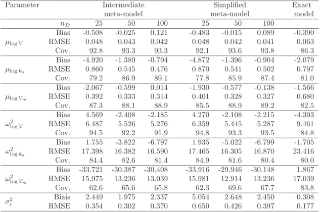
nD 25 50 100 25 50 100 µlogV Bias -0.508 -0.025 0.121 -0.483 -0.015 0.089 -0.390 RMSE 0.048 0.043 0.042 0.048 0.042 0.041 0.063 Cov. 92.8 93.3 93.3 92.1 93.6 93.8 86.3 µlogka Bias -4.920 -1.389 -0.794 -4.872 -1.396 -0.904 -2.079 RMSE 0.860 0.545 0.476 0.870 0.541 0.502 0.797 Cov. 79.2 86.9 89.1 77.8 85.9 87.4 81.0 µlogVm Bias -2.067 -0.599 0.014 -1.930 -0.577 -0.138 -1.566 RMSE 0.392 0.333 0.314 0.401 0.328 0.327 0.680 Cov. 87.3 88.1 88.9 85.5 88.9 89.2 82.5 ω2 logV Bias 4.569 -2.408 -2.185 4.270 -2.108 -2.215 -4.393 RMSE 6.487 5.526 5.276 6.359 5.445 5.287 9.461 Cov. 94.5 92.2 91.9 94.8 93.3 93.5 84.8 ω2 logka Bias 1.755 -3.822 -6.797 1.935 -5.022 -6.799 -1.705 RMSE 17.398 16.382 16.590 17.465 16.305 16.870 23.416 Cov. 84.4 82.6 81.4 84.9 81.6 80.4 80.0 ω2 logVm Bias -33.721 -30.387 -30.408 -33.916 -29.946 -30.148 1.867 RMSE 15.975 13.236 13.039 15.981 12.914 13.236 17.039 Cov. 62.6 65.6 65.8 62.3 69.6 67.7 83.8 σ2 ǫ Biais 2.449 1.975 2.337 5.054 2.648 2.450 0.308 RMSE 0.354 0.302 0.370 0.650 0.426 0.397 0.177 Table 1: Michaelis-Menten pharmacokinetic simulations: relative bias (%), relative
MSE (%) and coverage rate (%) computed over 1000 simulations, with the intermediate meta-, the simple meta- and the exact mixed models. Meta-models are built with either nD = 25, nD = 50 or nD = 100 design points. Coverage rate (Cov.) is the coverage
rate of the95%confidence interval based on the stochastic approximation of the Fisher matrix.
the exact likelihoodp(y;θ)and the maximum of the approximate likelihoodspD(y;θ),
¯
pD(y;θ)orp˜D(y;θ)can be as small as we want, as soon as the designDis rich enough.
7
Simulation study
The objective of this study is to compare the main statistical properties of the estima-tion with the mixed meta-models and compare them to the exact mixed model. Two examples are illustrated below, using standard ODE pharmacokinetics (PK) models.
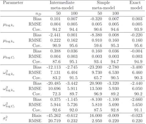
Parameter Intermediate Simple Exact meta-model meta-model model
nD 50 100 50 100 µlogke Bias 0.101 0.007 -0.320 0.007 0.003 RMSE 0.004 0.005 0.005 0.005 0.005 Cov. 94.2 94.4 90.6 94.6 93.9 µlogka Bias -2.441 0.001 -8.380 0.008 -0.220 RMSE 0.222 0.162 0.910 0.160 0.160 Cov. 90.9 95.6 59.6 95.3 95.6 µlogCl Bias 0.388 0.036 0.160 0.036 -0.004 RMSE 0.004 0.003 0.003 0.003 0.003 Cov. 87.6 95.1 93.4 94.7 94.9 ω2 logke Bias -12.113 -2.745 -23.200 -2.780 -3.400 RMSE 7.131 6.404 9.730 6.530 6.460 Cov. 83.2 91.5 65.7 90.5 90.3 ω2 logka Bias -20.485 -3.442 20.900 -3.320 -2.440 RMSE 10.696 5.911 13.500 5.930 6.050 Cov. 72.3 89.7 96.9 89.2 90.2 ω2 logCl Bias 0.375 -1.145 -8.100 -1.100 -2.660 RMSE 5.944 5.726 5.810 5.690 5.650 Cov. 92.6 92.0 87.5 92.8 91.1 σ2ǫ Biais -45.262 -0.612 16.000 -0.009 -0.023 RMSE 20.719 0.232 2.950 0.220 0.220
Table 2: One compartment simulations: relative bias (%), relative MSE (%) and cover-age rate (%) computed over 1000 simulations, with the intermediate meta-, the simple meta- and the exact mixed models. Meta-models are built with either nD = 50 or
nD = 100design points. Coverage rate (Cov.) is the coverage rate of the 95%
7.1
Michaelis-Menten pharmacokinetic model
7.1.1 Simulation settingsLet us now consider a one-compartment pharmacokinetic model, first order absorption and Michaelis Menten elimination. A doseD of a drug is given to a patient by intra-venous bolus. The concentration of the drug in the body along time in then described by the following ordinary differential equation
df dt =− Vm·f km+f +ka· D V ·exp(−ka·t), f(t0) = 0
whereV is the volume of distribution,Vmis the maximum elimination rate (in amount
per time unit),kmis the Michaelis-Menten constant (in concentration unit) andkais the
absorption constant. We consider logkm as fixed to−2.5. The individual parameter
ψ consists in logV, logka and logVm. We assume a Gaussian distribution on the
logarithm of these parameters with mean(µlogV, µlogka, µlogVm) = (2.5,1,−0.994)and a diagonal covariance matrix with terms (ω2
logV, ωlog2 ka, ω 2
logVm) = (0.09,0.09,0.09). Then a homoscedastic additive error model is simulated with a standard errorσε= 0.1.
We implement the four algorithms: SAEM on the original mixed model, SAEM on the complete, intermediate and simple mixed meta-model. For the meta-model SAEM algorithms, we use successivelynD= 25,nD= 50andnD= 100number of points in the
design of experiments for the Gaussian process emulator. The covariance is Gaussian, and the regression functions H are linear functions. More sophisticated choices in the regression functions and in the kernel can be made. However, our goal in this section is to illustrate in a quite simple case the efficiency of the combination of the Gaussian process emulation with the SAEM-MCMC algorithm. In the pre-computation step, for a given value ψ, the ODE solver providesf(t, ψ)for each time of measurement. Thus, the design of numerical experiment is only built over the values of ψ and not t. We have compared two approaches one where t is considered as an additional input and the other where a meta-model is built for each timet. Based on the comparison of the quality of the approximations, we have kept the second one which is quite simple to deal with. However, more sophisticated approaches can be tested (see Rougier, 2008, for a review). The approximation is built over the domain: [1.6; 3.3]forlogV,[0; 2.1]for
logkaand[−1.6;−0.3]forlogVm. The starting values for the parameters areµb(0)logV = 2,
b µ(0)logka= 0.5,bµ (0) logVm =−0.5,bω 2(0) logV =bω 2(0) logka=ωb 2(0) logVm = 0.1andσb (0) ε = 0.3. 7.1.2 Results
The computation times for one run of SAEM (100 iterations of SAEM, with 15 iterations of MCMC at each SAEM iteration) were the following: around 15 min for the exact mixed model (requiring solving the ODE at each iteration of MCMC), around 30 min for the complete mixed meta-model with nD = 50(requiring inverting the C(t,ψ)at
each iteration of MCMC), around 80 sec for the intermediate model and 30 sec for the simple one. Therefore, in the following, we only present the results for the exact mixed model (as a benchmark) and the intermediate and simple mixed meta-models.
Relative bias and relative root mean square error (RMSE) are computed for each pop-ulation parameter from 1000 replications and presented in Table 1. The95%coverage
rates correspond to the coverage rate of the confidence interval on parameters based on the stochastic approximation of the Fisher Information matrix. In this example, the two meta-models have good performances even with only 25 points in the design of experiments and increasing nD decreases the bias. The parameter ωlogVm is biased when using a meta-model (whatever nD) while it is not with the exact model. This
may be due to the error of approximation that is not completely taken into account.
7.2
First order pharmacokinetic model
7.2.1 Simulation settings
Let us consider a one-compartment PK model with first order absorption and elimina-tion, with a doseDof a drug. The concentration of the drug in the body along time in then described by the following ordinary differential equation
df dt =D
kake
Cl
exp(−kat)−kef, f(t0) = 0
where ka and ke are the absorption and elimination constants, Cl is the clearance.
We consider the PK parameters of theophyllin (Pinheiro and Bates, 2000): logke =
−2.52, logka = 0.4, logCl = −3.22. One dataset of 36 patients is simulated with a
dose D=6mmol and measurements at timet= 0.25,0.5,1,2,3.5,5,7,9,12hours. The random effects were simulated assuming a Gaussian distribution for the logarithm of the parameters with a diagonal variance-covariance matrix Ωwith the following diagonal elements: ω2
logke =ω 2
logka=ω 2
logCl= 0.01. Then a homoscedastic additive error model is simulated with a standard errorσε= 0.1.
The same SAEM algorithms were run as in the first example. The Gaussian process emulators were built withnD= 50andnD= 100points, linear regression functions and
a Gaussian covariance kernel, in the same fashion as in subsection 7.1.1. The domain where the approximation is built is[−4;−1]forlogke,[0; 2]forlogka and[−4.5; 2]for
logCl. The starting values for the parameters areµ(0)logke =−3,µ (0) logka= 1,µ (0) logCk =−3, ω2(0)logke =ω 2(0) logka=ω 2(0) logCl= 0.1 andσ (0) ε = 0.3. 7.2.2 Results
The computation times are the same as before. Relative bias, relative RMSE and cov-erage rate computed from 1000 replications are presented in Table 2. When the design of numerical experiments in the pre-computation step has 100 points, the estimates obtained with the mixed meta-models have similar performance to the ones obtained with the exact mixed model. With only50points in the design, the estimates with the mixed meta-models are less accurate, especiallyσεwith the intermediate mixed model.
There is a clear improvement of the quality of the estimates with the intermediate mixed meta-model for the parameters concerning the means. Recall that the simple mixed meta-model neglects the approximation of the functionf. Therefore, taking into account the errors of the approximation of the Gaussian process emulator in the model prevents from a systematic bias in the estimates. However, since the correlation be-tween the Gaussian process emulator approximation errors are set to zero for the sake
of simplicity, the estimation ofσε may be less accurate but usually this parameter if of
less interest.
8
Concluding remarks
In the case of a mixed model where the regression function is a non-analytical solution of an ODE or of a PDE, we proposed to build a so-called meta-model which is obtained thanks to a pre-computation step. It consists in running the ODE/PDE solver on a well chosen design of numerical experiments. Once this meta-model is obtained, we use it as a surrogate of the regression function in the estimation procedure which is based on a SAEM-MCMC algorithm. We derived three mixed meta-models depending on whether the additional source of uncertainty due to the approximation by the meta-model is taken into account totally, partially or not at all (complete, intermediate and simple mixed meta-model). In the complete mixed meta-model, there is a full covari-ance matrix accounting for dependencies induced by the meta-modeling errors which slows down the SAEM-MCMC algorithm. That is why we have renounced to test it in the simulation study. Further works are needed to design MCMC algorithm adapted to this case of non-independent individuals. In the intermediate and simple mixed meta-model, the individuals are still independent thus the SAEM-MCMC algorithm does not suffer from any computational burden. We showed examples where even with a very few design points for the meta-model approximation, the estimation results are very satisfactory. We also showed an example where the intermediate meta-model improves the quality of the estimates of the parameters especially those accounting for the mean of the population parameters.
Since the quality of the approximation provided by the meta-model directly depends on the density of the numerical design of experiments in the neighborhood of the input where the approximation is made, a sequential strategy for building an adaptive design reinforcing the meta-model where the SAEM-MCMC algorithm identifies likely region for the parameters should improve the estimates. However, this strategy would make the Markov property in the SAEM-MCMC procedure no longer to be valid. Therefore, there are theoretical questions which will be interesting to solve in order to ensure guarantees in this case.
Acknowledgements
Adeline Samson has been supported by the LabEx
PERSYVAL-Lab (ANR-11-LABX-0025-01). Les recherches menant aux présents ré-sultats ont bénéficié d’un soutien financier du septième programme-cadre de l’Union européenne (7ePC/2007-2013) en vertu de la convention de subvention n 266638.
References
Barbillon, P., Celeux, G., Grimaud, A., Lefebvre, Y., and Rocquigny, E. D. (2011). Nonlinear methods for inverse statistical problems. Computational Statistics & Data
Analysis, 55(1):132 – 142.
Chatterjee, A., Guedj, J., and Perelson, A. S. (2012). Mathematical modelling of HCV infection: what can it teach us in the era of direct-acting antiviral agents? Antivir Ther, 17(6 Pt B):1171–1182.
Davidian, M. and Giltinan, D. (1995). Nonlinear models to repeated measurement data. Chapman and Hall.
Delyon, B., Lavielle, M., and Moulines, E. (1999). Convergence of a stochastic approx-imation version of the EM algorithm. Ann. Statist., 27:94–128.
Dempster, A., Laird, N., and Rubin, D. (1977). Maximum likelihood from incomplete data via the EM algorithm. Jr. R. Stat. Soc. B, 39:1–38.
Donnet, S. and Samson, A. (2007). Estimation of parameters in incomplete data models defined by dynamical systems. J. Statist. Plann. Inference, 137:2815–2831.
Fang, K., Li, R., and Sudjianto, A. (2005). Design and Modeling for Computer Experi-ments (Computer Science & Data Analysis). Chapman & Hall/CRC.
Fu, S., Celeux, G., Bousquet, N., and Couplet, M. (2014). Bayesian inference for inverse problems occurring in uncertainty analysis. International Journal for Uncertainty Quantification.
Grenier, E., Louvet, V., and Vigneaux, P. (2014). Parameter estimation in non-linear mixed effects models with SAEM algorithm: extension from ODE to PDE. ESAIM: Mathematical Modelling and Numerical Analysis.
Guedj, J., Thiébaut, R., and Commenges, D. (2007). Maximum likelihood estimation in dynamical models of HIV. Biometrics, 63:1198–2006.
Johnson, M. E., Moore, L. M., and Ylvisaker, D. (1990). Minimax and maximin distance designs. Journal of Statistical Planning and Inference, 26(2):131 – 148.
Koehler, J. R. and Owen, A. B. (1996). Computer experiments. InDesign and analysis of experiments, volume 13 of Handbook of Statist., pages 261–308. North-Holland, Amsterdam.
Kuhn, E. and Lavielle, M. (2005). Maximum likelihood estimation in nonlinear mixed effects models. Comput. Statist. Data Anal., 49:1020–1038.
Lavielle, M., Samson, A., Fermin, A., and Mentre, F. (2011). Maximum likelihood estimation of long term HIV dynamic models and antiviral response. Biometrics, 67(1):250–259.
Lophaven, N., Nielsen, H., and Sondergaard, J. (2002). DACE, a matlab kriging toolbox. Technical Report IMM-TR-2002-12, DTU. Available to : http://www2.imm.dtu.dk/ hbn/dace/dace.pdf.
Louis, T. A. (1982). Finding the observed information matrix when using the EM algorithm. Journal of the Royal Statistical Society. Series B, 44(2):226–233.
Pinheiro, J. and Bates, D. (2000).Mixed-effect models in S and Splus. Springer-Verlag. Prasad, N. and Rao, J. N. K. (1990). The estimation of the mean squared error of small-area estimators. Journal of the American Statistical Association, 85:163–171. Ribba, B., Kaloshi, G., Peyre, M., Ricard, D., Calvez, V., Tod, M., Cajavec-Bernard,
B., Idbaih, A., Psimaras, D., Dainese, L., Pallud, J., Cartalat-Carel, S., Delattre, J., Honnorat, J., Grenier, E., and Ducray, F. (2012). A tumor growth inhibition model for low-grade glioma treated with chemotherapy or radiotherapy. Clin Cancer Res, 18:5071–5080.
Rougier, J. (2008). Efficient emulators for multivariate deterministic functions. Journal of Computational and Graphical Statistics, 17(4):827–843.
Sacks, J., Schiller, S. B., Mitchell, T. J., and Wynn, H. P. (1989). Design and analysis of computer experiments. Statistical Science, 4:409–435.
Samson, A., Lavielle, M., and Mentré, F. (2007). The SAEM algorithm for group com-parison tests in longitudinal data analysis based on non-linear mixed-effects model.
Stat. Med., 26(27):4860–4875.
Santner, T. J., Williams, B., and Notz, W. (2003). The Design and Analysis of Com-puter Experiments. Springer-Verlag.
Schaback, R. (1995). Error estimates and condition numbers for radial basis function interpolation. Advances in Computational Mathematics, 3(3):251–264.
Schaback, R. (2007). Kernel-based meshless methods. Technical report, Institute for Numerical and Applied Mathematics, Georg-August-University Goettingen.
Wei, G. C. G. and Tanner, M. A. (1990). Calculating the content and boundary of the highest posterior density region via data augmentation. Biometrika, 77(3):649–652. Wolfinger, R. (1993). Laplace’s approximation for nonlinear mixed models.Biometrika,
80(4):791–795.
Wu, H., Huang, Y., Acosta, E., Rosenkranz, S., Kuritzkes, D., Eron, J., Perelson, A., and Gerber, J. (2005). Modeling long-term HIV dynamics and antiretroviral response: effects of drug potency, pharmacokinetics, adherence, and drug resistance. Journal
of Acquired Immune Deficiency Syndromes, 39:272–283.
Wu, Z.-M. and Schaback, R. (1992). Local error estimates for radial basis function interpolation of scattered data. IMA J. Numer. Anal, 13:13–27.
Appendix
Proof of proposition 3
We have |p(y;θ)−p˜D(y;θ)| ≤ Z |p(y|ψ;θ)−p˜D(y|ψ;θ)|p(ψ)dψ.Therefore, we start by studying|p(y|ψ;θ)−p˜D(y|ψ;θ)|: (2πσε2)n tot/2|p( y|ψ;θ)−p˜D(y|ψ;θ)| = exp − 1 2σε2 X ij (yij−f(tij, ψi))2 −exp − 1 2σ2ε X ij (yij−mD(tij, ψi))2 = exp − 1 2σε2 X ij (yij−f(tij, ψi))2 ! × 1−exp − 1 2σ2 ε X ij (yij−mD(tij, ψi))2−(yij−f(tij, ψi))2 ≤ 1−exp − 1 2σ2 ε X ij f(tij, ψi)−mD(tij, ψi))(2yij−f(tij, ψi)−mD(tij, ψi) .
Under the assumption that the functions f and mD are uniformly bounded on the
support of ψ, there exists a constant Cy which is uniform according to ψ such that
|2yij −f(t, ψ)−mD(t, ψ)| ≤Cy. Proposition 1 implies that the approximation error
due to the metamodel|f(tij, ψi)−mD(tij, ψi)|is controlled by inequality (8):
|f(tij, ψi)−mD(tij, ψi)| ≤ kfkHKGK(aD). Then there exists a constantCy depending only on ysuch that
(2πσ2ε)ntot/2|p(y|ψ;θ)−p˜D(y|ψ;θ)| ≤Cy ntot 2σ2 ε kfkHKGK(aD). Finally |p(y;θ)−p˜D(y;θ)| ≤ Cy (2πσ2 ε)ntot/2 ntot 2σ2 ε kfkHKGK(aD).
8.1
Proof of proposition 4
We study the distance between the two likelihoodspDandp˜D. As in Proposition 3, we
start by studying |pD(y|ψ;θ)−p˜D(y|ψ;θ)|. We consider two Gaussian distributions
whenP(yij−mD(tij, ψi))2= 0. This yields (2π)ntot/2|p D(y|ψ;θ)−p˜D(y|ψ;θ)| ≤ 1 σntot ε −p 1 |σ2 εIntot+CD| = 1 σntot ε 1− σ ntot ε |σ2 εIntot+CD| 1/2 ≤ 1 σntot ε 1− σntot ε (σ2 ε+ntot1 P ijCD(tij, ψi;tij, ψi))ntot/2 ≤ 1 σntot ε 1− 1 (1 +σ21 εntot P ijCD(tij, ψi;tij, ψi))ntot/2
where we use that the determinant, as a product of eigen values, is smaller than a function of the trace of the matrix. Thus, the sum is over the diagonal of the matrix
CDi.e. the sum of the variances. Then, we obtain that there exists a constantC such
that |pD(y|ψ;θ)−p˜D(y|ψ;θ)| ≤ C 1 σntot ε 1 2σ2 ε X ij CD(tij, ψi;tij, ψi) ≤ C(2π)ntot/2 ntot σnεtot+2 GK(aD)
where the last inequality holds using Proposition 1. Finally, we obtain
|pD(y;θ)−p˜D(y;θ)| ≤Cy
ntot
σnεtot+2
GK(aD).