The cost for the default of a loan Linking theory and practice

The cost for the default of a loan

– Linking theory and practice –

By

Rafael Weissbach & Philipp Sibbertsen

Department of Statistics

University of Dortmund

May 17, 2004

∗_{address for correspondence: Rafael Weissbach, Institute for Business and Social}

Statis-tics, Faculty of StatisStatis-tics, University of Dortmund, 44221 Dortmund, Germany, email: [email protected], Fon: +49/231/7555419, Fax: +49/231/7555284. Supported by DFG, SFB 475 “Reduction of Complexity in Multivariate Structures”, project B1.

Abstract

When calculating the cost of entering into a credit transaction the pre-dominant stochastic component is the expected loss. Often in the credit business the one-year probability of default of the liable counterpart is the only reliable parameter. We use this probability to calculating the exact ex-pected loss of trades with multiple cash flows. Assuming a constant hazard rate for the default time of the liable counterpart we show that the methodol-ogy used in practice is a linear Taylor approximation of our exact calculus. In a second stage we can generalize the calculation to arbitrary hazard rates for which we prove statistical evidence and develop an estimate from historical data.

1

Introduction

National authorities regulate the business of trading (derivative) financial instruments with respect to the market risk. The international ”minimal re-quirements for trading” which were evolved in the past ten years have been translated into national law (e.g. the ”Mindestanforderungen f¨ur das Be-treiben von Handelgesch¨aften” (MaH) in Germany). Similar approaches to managing credit risk arise nowadays in the capital accords at the Bank of International Settlement (named Basle II, see Basel Commitee on Banking Supervision (2003)). The international banking industry together with the Bank of International Settlement believe that further regulation is necessary for credit risk as the volume of products which can trade credit risk has rapidly increased. In recent years a standardization in documentation, e.g. for credit default swaps (see ISDA (2002) and ISDA (2003)) has enabled such growth. The leverage of risk is dramatically higher than in the lend-ing business. However, the lendlend-ing business is now in competition with the investment banking. Owing to the high risks in derivative products their risk management, due to regulatory, but also voluntary, requirements uses

sophisticated methods of primarily stochastic and statistical nature. As a consequence, the lending business now can and needs to adopt the method-ology developed. At a first stage we derive accurate formulae for the expected loss, constituting the primary stochastic cost when lending. To this end, we show that the loss arising from a loan is a stochastic (jump) process.

The repayment of a loan by a debtor can be viewed as cash flow seriesati

at the points in time t0 < t1 < . . . < tn = T. Positive payments symbolize

flows from the debtor to the creditor, negative payment from the creditor to the debtor. It is typical in practise to fix the payment dates and payment heights when the contract is negotiated. We refrain from modelling random payment dates and heights. The transaction starts with the granting of the notional of the loan at the time t0, w.l.o.g. today, 0, and ends with maturity

T. We assume that all in-coming and out-going cash flows at one point in time can be netted. Typically, in the lending business we have a loan with only positive cash flows after the initial donation of the notional. The cash flows of that type of loan are visualized in Figure 1. When being contacted by a potential debtor at first time the creditor needs to calculate the cost in order to decide whether and if at which rate to lend.

The loss of the trade is not known in advance and will depend on the time of default, i.e. the survival time. The analysis of survival times is well established in the literature (see e.g. Aalen (1978), Andersen et al. (1993), Borgan (1997), Fleming and Harrington (1991), Hougaard (2001), Kalbfleisch and Prentice (1980) and Lee (1992)).

W.l.o.g. we suppress the effect of time-value of money and think of the

ati’s as derived from ˜ati’s by discounting with the current risk-free interest

rate curve, r(s) (e.g. Euribor). That means we assume that

ati = ˜atidfti,

withdftias discount factor for a cash flow at timeti, namely,dfti =e

r(ti)ti. For

the instantaneous forward interest rate curve rf_{(s) = lim}

ds→0(rf(s, s+ds))

the discount factor is dfti =e

Rti

t1 tn =T

at1

atn

Figure 1: Discounted future cash flows of transaction

The paper is structured as follows. For the sake of clarity we use a single payment loan (bullet) at first and afterwards a realistic multi-payment loan. The implicit two-by-two table of cases together with the assumption of constant and non-constant hazard rates is covered for both constant hazard rate cases with Section 2. For brevity we leave out the case of non-constant hazard rate and bullet loan and discuss the most complex case of the multi-payment loan under a non-constant hazard rate in Section 3. The latter investigation is preceded by an argument in favor of a non-constant hazard rate. In Section 4 we consider the implications of the developed costing for the pricing of loans.

2

Constant risk profile

The maturity of loans is rarely one year exactly. To calculate the expected loss of such trades we need to deduce a model for the default of the li-able counterpart from the one-year probability of default (denoted by PD1

throughout the text). If we have no specific model for the default behavior of the debtor we may assume that its tendency to default over time is constant. That means we assume for the default time τ: P(τ ∈[t, t+dt]|τ ≥ t) ≡α. The constant hazard rate α is equivalent to an exponentionally distributed default time and hence the PD1 determines the distribution parameterα by

the relationship

F(1) = 1−e−α ₍₁₎

(see e.g. Lee (1992)) where F(t) :=P(τ ≤t). Any PD of the debtor is given by F(t) = 1−e−αt_.

2.1

Expository model: A single payment loan

In view of the situation of a creditor who lends one unit of currency or equiv-alently buys a bond with unit notional the creditor is prepared to reduce the initial amount of lending by the cost of expected loss. Our aim is to calculate the expected loss. In the current paragraph we will refrain from including discounting factors which arises from the supply-and-demand equilibrium of interest rates to clarify components of the interest rate which arises from default.

The total expected loss costs are in practice often calculated for the loan with maturity T with the help of (1) as

T ×F(1) =T(1−e−α). (2) The stated procedure is underpinned statistically by the Bernoulli model for the one-year default. However, for multi-year transactions the notion is not exact anymore because the loss is not the sum of T independent trials. For transactions where T is not natural, e.g. for short transaction with maturity below one year, the notion even fails. We prefer to model the loss now in a continuous fashion. Imagine a creditor ”watching” his loan through

time t starting at the beginning of the granted loan in t0 = 0 (ending in T). The loss situation for the creditor for 0 ≤t≤T is given by the function

Lt:=I{τ≤t}

whereIconditiondenotes the indicator function, i.e. is 1 if theconditionis true

and 0 else. From a mathematical point of view Lt is a stochastic process.

We require a probability space (Ω, P,F), an increasing filtration of sub-σ -algebras Ft ⊂ F and Lt to be adapted to the filtration. It is well known

that any stochastic process can be decomposed into a trend-type component, named ”compensator”, and a martingal.

In order to determine the compensator, it should be noted that

E(dLt|Ft−) =I{τ≥t}P(τ ∈[t, t+dt]|τ ≥t) =I{τ≥t}α

| {z }

:=λ(t) dt

with intensity process λ(·).

Hence, we have Lt = Λt+Mt with Λt =

Rt

0 λ(s)ds (see Andersen et al.

(1993)) as cumulative intensity. As L0 = 0 and Λ0 = 0, we have E(MT) =

E(M0) = 0, so that E(LT) = E(ΛT) +E(MT) = Z T 0 EI{τ >s}αds= Z T 0 f(s)ds =F(T) = 1−e−αT_{. (3)}

Remark 1. The unit notional was chosen for pure convenience. For a generalization to any (known) cash flowA, multiply the expected loss (3) by the latter. So far, our behavioral model has been that the counterparts agree on the exchange of the amountA, the notional, inT. Thereafter, the creditor reduces the initial payment to the debtor by the cost for the expected loss and hence pays out Ae−αT_{. However, to regain the notional at the maturity}

of a trade is common only in the bond market. For loans, the notional is usually granted initially and returned including interest at the timeT. (The latter modality is still a simplification. Usually, short running loans have

aggregated compensation at maturity called ”bullet” structure. For longer maturities it is common to pay interest periodically. We will cover this case later.) For the application of (3) to a loan with final compensation think of the final payment A as the compensation for a loan with notionalAe−αT_{. If}

now, instead of the final paymentA, the initially granted notionalB is fixed

A (seen as redemption including costs for the expected loss) is

A=BeαT. (4)

Formula (4) demonstrates that the accounting for the expected loss is similar to continuous compounding of A with interest rateα (see Hull (2000)). The latter is long known in the pricing of derivative products subject to credit risk.

Remark 2. To compare the exact expected loss costs (3) with the sim-plified practical approach (2) one could consider the difference

DT :=T(1−e−α) +e−αT −1.

It can be easily seen that the roots of DT, i.e. the maturities where the

simplified approach is exact, are T = 0 and T = 1. To examine the behavior of DT in more detail we consider the first derivative

D0T = (1−e− α

)−αe−αT.

We obtain the local extremes by solving D0

T = 0. This is the case for T0 = −1

αln(

1−e−α

α ). The second derivative ofDT isD

00

T =α2e−αT being positive at

T =T0 proving that the differenceDT has exactly one local minimum. This

proves that DT is decreasing for T < T0 and increasing for T > T0 showing

that DT is negative for 0 < T < 1 and positive for T > 1. Therefore, the

simplified calculation understates the costs for maturities under one year and overstates the costs for maturities over one year where the benefits from our approach increases exponentially. Numerical root finding reveals that the cost of the market method values 10% higher compared with the realistic cost in the case of a PD1 of 1% at T = 20.

Given the fact that T0 is near to zero for all 0< α < 1, which holds for the realistic cases of 0 < P D1 <0.2, our approach gives comparable values to the common market practice for T <1 (year).

Remark 3. Although we are talking about the expected loss, it might be worthwhile to consider its variance. As the loss Lt is a Bernoulli variable

with expectation 1−e−αt _{the variance is (1−e}−αt_)e−αt_{. Interestingly, the}

variance is approximately e−αt _{for large t}1 _{and approximately 1−e}−αt _for

small t2_.

2.2

The multiple payment loan

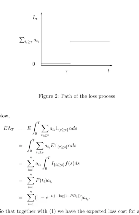
In the general cash flow structure laid out in Section 1 the loss is the stochas-tic process Lt= 1{t≥τ} X ti≥τ ati = 1{t≥τ} n X i=1 1{τ≤ti}ati.

The process is depicted in Figure 2.

To calculate the compensator we calculate again the expected incremental changes E(dLt| Ft−) = 1{τ≥t} X ti≥t atiE(1{τ∈[t,t+dt]} | Ft−) = 1{τ≥t} X ti≥t atiα | {z } =:λ(t) dt (5)

where λ(·) is the intensity process. To calculate the expected loss for timeT

in the stochastic calculus we need to calculate the expected trend at time T

because

ELT =EΛT.

1₍₁₋e−αt)e−αt=e−αt−e−2αt≈e−αt

-6 τ t Lt 0 P ti≥τati p `

Figure 2: Path of the loss process

Now, EΛT = E Z T 0 X ti≥s ati1{τ≥s}αds = Z T 0 X ti≥s atiE1{τ≥s}αds = n X i=1 ati Z T 0 I{ti≥s}f(s)ds = n X i=1 F(ti)ati = n X i=1 (1−e−ti(−log(1−P D1))_)a ti.

So that together with (1) we have the expected loss cost for a loan with one final compensation:

Theorem 2.1 The expected loss of a loan with maturity T and contractual payment of ati at dates ti, i= 1, . . . , n, to a liable counterpart with constant

instantaneous risk to default determined by the one-year probability of default PD1 is given by E(LT) = n X i=1 (1−(1−P D1)ti)ati.

2.3

Taylor approximation

In accordance with the calculation of the expected loss for a single payment loan (2) in practice a simple approach is common for multi-payment loans: Use the given one-year probability of default PD1, apply it to each year

in which the loan is granted and add the yearly costs PD1 × notional. It

is assumed that the hazard rate is constant. In fact, the procedure is an analytic approximation of the exact cost given in Theorem 2.1, because of

Theorem 2.2 Under the notion of the preceding sections and the assumption of a constant hazard rate it holds:

ELT ≈ n

X

i=1

P D1tiati.

The equality holds for P D1 = 0.

Proof: Expand the coefficient in Theorem 2.1 with respect to the variable PD1 at 0 (because default tends to be rare in lending):

1−(1−P D1)ti = ∞ X ν=1 (−1)ν+1 ti! (ti−ν)! P D₁ν.

If we use a linear approximation we have 1−(1−P D1)ti

=tiP D1.

Thus, we have shown that the conventional calculation is a Taylor approxi-mation, by only using the linear coefficient.

We would like to emphasize that the business implications are noticeable with an example which will be used repeatedly in the text. Consider a 10 year loan of 100 million Euro to a counterpart with one-year PD of 1%. We consider the case of constant annuities, i.e. annual payments of 10 million to pay back the debts. The expected loss with respect to the method, which is given in Theorem 2.2, is 5.5 million Euro, or 5.5%. Whereas the expected loss in the full model of Theorem 2.1 is 5.34 million Euro - or 5.34%, the user of the market method given in Theorem 2.2 collects 160,000 Euro too much from the counterpart. The difference of 16 basis points is huge from an investment banking perspective, especially when looking at liquid markets like the Swap market. However, the quantity is not easy to assess because it is not denoted on an annual basis. The interest needs distribution over ten years. It is not possible to divide the amount by ten in the case of the ten-year loan because the future cash flows are subject to default, and, hence less valuable. The equilibrium premium mark-up is the topic of the last Section 4.

3

Variable risk profile

Often in practice it is argued that the one-year PD1 cannot be applied to

all time periods as done in the latter section. In terms of the hazard rate the assumption of a constant rate is unrealistic. We would like to investigate this assumption with inferential statistics. The assumption is difficult to assess when using annual cohort data as supplied, for example, by the federal statistical offices in Germany. The data required for such assessment needs to be continuous (as in Lando and Skødberg (2002)). However, in contrast to the latter article we do not use Moody’s data for the reason that each bank has its own data and must rely on it to decide on the behavior of its portfolio of counterparts. Especially in Europe where many counterparts are not being rated by agencies the Moody’s data pool seems unapplicable. And,

in fact, banks do maintain evidence of their history of default on a continuous basis, subsequently they know the default time exactly. We use such internal data, in a modified version, as supplied by a cooperating large international bank. From a statistical point of view we need a test of the null hypothesis of a constant hazard rate first given the one-year PD1.

3.1

Test for constant risk

In fact, the question arises which model for the hazard rate to apply. The assumption of a constant rate is certainly appealing in terms of simplicity. However, the question is: Could we have done better knowing that the haz-ard was constant? The answer is ‘yes’. An efficient estimate for α could have been constructed for the model where the survival times are exponen-tially distributed with parameter α. The maximum likelihood estimate from a sample X1, . . . , Xn of identically independently distributed random

vari-able is known to be n/Pn_i=1Xi and this is certainly a good estimate. Note

that 1/α is the expectation of the exponential distribution. The point is, rather, how can we decide whether the hazard rate is constant? We would like to integrate the important issue of missing data at this stage. As the interesting event is ”default after amendment to the portfolio” the time of initialization of the trade must be seen as the origin of the random variable ”default time”. The censoring that can occur is then right-censoring as the event may not be observed due to the termination of trade without default (or discontinued rating). In any type of survival analysis and especially in assessing the credit risk, right-censored observations arise from ”good” risk, which means that counterparts do not default while being under investiga-tion. These observations have to be incorporated into the estimation and testing of the hazard rate because neglecting them would result in serious bias, in this case overstatement of the risk.

Employing the common notation for censored data, we define that then

either to the survival timesTi or the censoring timesCi and thatδi =I{Xi=Ti}

indicates the censoring fori= 1, . . . , n. Ordering of the censoring indicators

δ(i) follows that of the corresponding observationsX(i).

In the statistical literature the test for constant hazard rate is known as ”one-sample log-rank test” (see Breslow (1975)). The test can by integrated into the context of counting processes (see Andersen et al. (1993)). We can assume the one-year PD1 to be known and, see (1), apply the test to the

hypothesis

H0 : α(t)≡ −log(1−P D1).

The asymptotically standard normal distributed test statistic is

V = N(pt)−E(t)

E(t) (6)

where N(t) := ]{i : Ti ≤ t, Ci = 1} is the number of uncensored defaults

until timetandE(t) :=−log(1−P D1)Pn_i=1Xi∧tis the expected number of

defaults in [0, t]. Usually, one uses for the argumentt the largest uncensored default time.

Study data In banks it is common practice to rate a counterpart once an engagement is committed. Ongoing regular rating (at least on an annual basis) is mandatory until the trade is matured. This data can be used to test the assumption of a constant hazard rate. Fortunately, from a busi-ness perspective, many of the engagements end without the observation of a default (time). We can model this missing data with the discussed right-censoring mechanism. We use a fictitious, although realistic, data set of 200 counterparts belonging to a homogeneous (minor) rating class with default or censoring times ranging from 7 days to 4.9 years. The censoring is 69.5%. A first impression of the data is given by the product-limit estimate in Figure 3 which was realized using SAS.

Figure 3. Kaplan-Meier estimate of the survival distribution function of the default time in the rating class.

We can use a kernel estimate of the hazard rate (see e.g. Sch¨afer (1986))

αn(t) = n X i=1 δ(i) n−i+ 1 1 bK X(i)−t b . (7)

to assess the assumption of a constant risk.

For an optimal choice of the bandwidth parameter we can use the selectors from the density estimation context (see Hjort (1991)). A recent summary of selectors can be found in Hall et al. (1991).

For our study data the hazard rate estimate programmed in SAS/IML is depicted in Figure 4. We restrict the display to 800 days because in the right tail no uncensored information is available which can cause the flat behavior of the survival distribution in Figure 3 and, hence, does not exhibit infor-mation for the derivative, roughly being the hazard rate. The bandwidth was chosen optimally with respect to the mean integrated squared error in the context of density estimation assuming a underlying normal distribu-tion. This method is sometimes referred to as ”rule of thumb”. (See for

example Silverman (1986) for the case of fixed bandwidth density estimation and Weissbach and Gefeller (2004) for the adaption of censored hazard rate estimation with the nearest neighbor bandwidth.) It can be seen that three modes seem to be present.

Figure 4. Kernel estimate of the hazard rate with nearest neighbor bandwidth and 23nearest neighbors.

To supplement the descriptive assessment of the hazard rate we use the constructed test (6) for inferential statistics.

We assume the rating to be well calibrated and use the one-year probabil-ity of the product-limit estimate of 38.7% as a one-year PD which is assumed to be known (see Figure 3). The maximum uncensored survival timetis 1.86 years and until then N(t) = 61 defaults occur. Under hypothesis with con-stant hazard rate the expected number is E(t) = 77. The test rejects the hypothesis at a level of 5% and, hence, strongly supports our judgement of a varying hazard rate. The p-value is 0.0340895.

In the following section we will generalize the calculation of the expected loss to the case of an (unknown) functional default behavior of the

counter-part.

3.2

The general loss process

We want to generalize the calculation in Section 2.2 from the constant hazard rate α to any hazard rate α(t). It should be noted that now

E(dLt|Ft−) =I{τ≥t}P(τ ∈[t, t+dt]|τ ≥t) =I{τ≥t}α(t)

| {z }

:=λ(t) dt

with intensity process λ(·).

Generalizing (5) we have E(LT) = 1{τ≥t}

P

ti≥tatiα(t)dt. Again, we have

achieved E(LT) =

Pn

i=1F(ti)ati where the cumulative distribution function

F(t) is no longer given by the exponential distribution but by the hazard function. By using here the discounting factors again, we have as a universal costing formula for the expected loss:

Theorem 3.1 The expected loss of a loan with maturity T and contractual payments of ˜ati at datesti and discount factorsdfti fori= 1, . . . , nto a liable

counterpart with risk of default parameterized by the hazard rate α(t)is given by E(LT) = n X i=1 (1−e−R₀tiα(s)ds_)˜a tidfti.

3.3

Estimation of the variable default risk

As we have seen from Theorem 3.1, the only stochastic parameter which is necessary to calculate the expected loss is the cumulative hazard rate

A(t) :=R₀tα(s)ds. An unbiased estimator of the latter is the Nelson-Aalen estimate (see Aalen (1978) and Nelson (1972)), which has been especially designed for right-censored observations

An(t) =

X

i:X₍i₎≤t

δ(i)

4

Pricing

In practice the expected loss cannot be collected at the beginning of the trade. However, when distributing the cost over the future cash flows they inhibit the possibility to fail. Assuming we want to calculate a constant surplus ε to the ati, the additional cash flow arising from the risk premium

is Pt = ε n X i=1 1{τ >ti}.

In order to compensate for the expected loss in Theorem 2.1, the expected premium needs to equal the expected loss. The expected premium E(PT)

is easily calculated as εPn_i=1e−R₀tiα(s)ds_{. The premium, also named ”credit}

spread”, which is paid constantly is subsequently

ε= Pn i=1(1−e− Rti 0 α(s)ds)˜a_t idfti Pn i=1e− Rti 0 α(s)ds . (9)

Remark 4. For the constant hazard rate the premium reduces to

ε= Pn i=1(1−(1−P D1)t i )˜atidfti Pn i=1(1−P D1)ti . (10)

For our example of the ten year loan with a 1% annual default probability, the εis 0.5639%, which adds up to 5.639 million if the counterpart fulfills all duties. This amount is slightly higher than the expected loss of 5.34 million due to the potential loss of parts of the premium when the counterpart default prior to the maturity of the trade. The easiest charge for the expected loss on an regular basis as indicated by the formula (2) for the the one-year loan would be 1% for all periods. This approach would almost double the exact credit spread (10 in our example.

Remark 5. From microeconomic theory we know that in competitive markets, as in the capital market, the supplier of capital has negligible impact on the price. However, proper pricing of the loan is not redundant for one

important reason. The price developed can be seen as a hurdle rate to the market price. If the credit spread in the market is above the hurdle rate (9) we safely enter into a deal, otherwise our risk perception is above the market’s and the investor should refrain from trading.

5

Summary

We have discussed the loss and its cost in terms of the expected loss of loans. We started with a loan with bullet payment and modelled the loss as stochas-tic jump process to derive a formula for the exact expected loss. Assuming a constant hazard rate of default for the counterpart, we showed that the standard practice in banking is a Taylor approximation of our result only by using the linear component. We have given evidence that the hazard rate may not be assumed to be constant and derive a formula which accounts for the cumulative hazard rate. Furthermore, we have showed how to estimate the latter from right-censored data. The techniques which we have applied generalize the calculation of the expected loss by using migration matrices as in Lando and Skødberg (2002) due to of the continuous nature which makes the assumption of a discrete cash flow structure such as for rating matri-ces redundant. We have integrated the cost of default into the interest rate charged by the investor as price building.

References

Aalen, O. (1978). Nonparametric estimation of partial transition probabilities in multiple decrement models. Annals of Statistics, 6:534–545.

Andersen, P., Borgan, Ø., Gill, R., and Keiding, N. (1993). Statistical Models Based on Counting Processes. Springer-Verlag New York.

capital accord, consultative document. Technical report, Bank for Inter-national Settlements.

Borgan, Ø. (1997). Three contributions to the encyclopedia of biostatistics: The nelson-aalen, kaplan-meier, and aalen-johansen estmators. Technical report, Department of Mathematics, University of Oslo.

Breslow, N. (1975). Analysis of survival data under the proportional hazards model. Internat. Statist. Rev., 43:45–58.

Fleming, T. and Harrington, D. (1991). Counting Processes and Survival Analysis. Wiley, New York.

Hall, P., Sheather, S., Jones, M., and Marron, J. (1991). On optimal data-based bandwidth selection in kernel density estimation. Biometrika, 78:263–269.

Hjort, N. (1991). Semiparametric estimation of the hazard rates. InAdvanced Study Workshop on Survival Analysis and Related Topics. NATO.

Hougaard, P. (2001). Analysis of Multivariate Survival Data. Springer, New York.

Hull, J. (2000). Options, Futures, and other Derivatives. Prentice-Hall, Upper Saddle River.

ISDA (2002). 2002 ISDA Master Agreement. Technical report, International Swaps and Derivatives Association Inc., New York.

ISDA (2003). 2003 ISDA Credit Derivatives Definitions. Technical report, International Swaps and Derivatives Association Inc., New York.

Kalbfleisch, J. and Prentice, R. (1980). The Statistical Analysis of Failure Time Data. John Wiley & Sons, New York.

Lando, D. and Skødberg, T. (2002). Analyzing rating transitions and rating drift with continuous observations. J Banking Finance, 26:423–444. Lee, E. (1992). Statistical Methods for Survival Data Analysis. John Wiley

& Sons, New York.

Nelson, W. (1972). Theory and applications of hazard plotting for censored failure data. Technometrics, 14:945–966.

Sch¨afer, H. (1986). Local convergence of empirical measures in the random censorship situation with application to density and rate estimators. An-nals of Statistics, 14:1240–1245.

Silverman, B. (1986). Density Estimation. Chapman & Hall, London. Weissbach, R. and Gefeller, O. (2004). A rule of thumb for the variable

bandwidth selection in kernel hazard rate estimation. Technical report, Department of Statistics, University of Dortmund.

SAS and SAS/IML are registered trademarks of SAS Institute Inc. Carry, NC, USA.