Intuitive Exploration of Multivariate Data

Intuitive Exploration of

Multivariate Data

Dissertation

zur

Erlangung des Doktorgrades (Dr. rer. nat.)

der

Mathematisch-Naturwissenschaftlichen Fakult¨

at

der

Rheinischen Friedrich-Wilhelms-Universit¨

at Bonn

vorgelegt

von

Daniel Paurat

aus

Duisburg

Bonn, 2017

Angefertigt mit Genehmigung der Mathematisch-Naturwissenschaftlichen Fakult¨at der Rheinischen Friedrich-Wilhelms-Universit¨at Bonn

1. Gutachter: Prof. Dr. Thomas G¨artner 2. Gutachter: Prof. Dr. Stefan Wrobel Tag der Promotion: 15.03.2017

Erscheinungsjahr: 2017

Daniel Paurat

University of Bonn

Department of Computer Science III and

Fraunhofer Institute for Intelligent Analysis and Information Systems IAIS

Declaration

I, Daniel Paurat, confirm that this work is my own and is expressed in my own words. Any uses made within it of the works of other authors in any form (e.g. ideas, equations, figures, text, tables, programs) are properly acknowledged at the point of their use. A full list of the references employed has been included.

Acknowledgements

I would like to express my sincere gratitude to Thomas G¨artner for the trust and for encouraging me to start this work, for the constant support throughout it, countless discussions and for being a great supervisor in general. Henrik Grosskreutz and Mario Boley for guiding me through the first year. Roman Garnett, Tam´as Horv´ath, Ulf Brefeld and Kristian Kersting for all the quality discussions. Michael Kamp for innumerable coffee and theory crafting sessions; I really enjoyed our talks a lot. The other PhD students at Fraunhofer institute from Thomas’ and Kristian’s research groups, namely Pascal Welke, Olana Missura, Dino Oglic, Katrin Ullrich, Anja Pilz, Fabian Hadiji, Babak Ahmadi and Mirwaes Wahabzada. Not to forget my awesome office mates Sandy Moons and Marion Neumann. All of you guys and some of the really inspiring students that I met over the last couple of years provided an exquisite environment for me to pursue my thesis. It was a great time for me and I certainly would drink work with all of you again!

I would also like to thank my parents Roland and Ute Paurat for the trust they granted me. My partner Stephanie H¨oppner for the freedom and the constant stream of motiva-tion, as well as our son Jakob for providing me the final reason to complete this work. Finally, I would like to thank all of my friends, who repeatedly had to endure my talks on data analysis, with a special reference to Sebastian Ginzel for the (sometimes much needed) discussions and talks. I owe all of you guys my deepest gratitude.

Part of this work was supported by the German Science Foundation (DFG) under the reference numbers ‘GA 1615/1-1’ and ‘GA 1615/1-2’.

Abstract

Approaching a dataset with an analysis question is usually not a trivial process. Apart from integrating, cleaning and pre-processing the data, typical issues are to generate and validate hypotheses, to understand which algorithms to apply, to estimate parameter settings and to interpret intermediate analysis results. To this end, it is often helpful to explore the data at first in order to find and understand its main characteristics, the driving influences, structures and relations among the data records, as well as revealing outliers. Exploratory data analysis, a term coined by John W. Tukey (Tukey, 1977), is

a loose set of methods, mostly of graphical nature, to summarize and understand the main characteristics of the data at hand. This work extends the set of exploratory data analysis methods by proposing several new methods that support the analyst in his, or her task of understanding the data. Over the course of this thesis, two conceptually different approaches are investigated.

The first approach studies pattern mining algorithms, a family of methods that find and report hypotheses which describe interesting sub-populations of the dataset to the analyst, where the interestingness is measured by different quality functions. As the results of pattern mining methods are interpretable by a human expert, these algo-rithms are often utilized to study a dataset in an exploratory way. Note that many pattern mining algorithms address the problem of finding a small set of diverse high quality patterns. To this end, this work introduces two new algorithms, one for relevant and one for ∆-relevant subgroup discovery. In addition an algorithmic framework for sampling patterns according to different pattern quality measures is introduced. The second approach towards exploratory data analysis leaves the discovery of interesting sub-populations to the analyst and enables him, or her to study a two dimensional pro-jection of the data and interact with it. A scatter plot visualization of the projected data lets the analyst observe the data collection as a whole and visually uncover interesting structures. Manipulating the locations of individual data records within the plot further enables the analyst to alter the projection angle and to actively steer the projection. This way relations among the data records can be set, or discovered and aspects of the data’s underlying distribution can be explored in a visual manner. Finding the according projections is not trivial and throughout this thesis three novel approaches are proposed to do so.

The thesis concludes with a synthesis of both approaches. Classical pattern mining algorithms often aim at reducing the output of patterns to a small set of highly interesting and diverse patterns. However, by discarding most of the patterns, a trade-off has to be made between ruling out potentially insightful patterns and possibly drowning the analyst in results. Combining interactive visual exploration techniques with pattern discovery, on the other hand, excels on working with larger pattern collections, as the underlying pattern-distribution emerges more clearly. This way, the analyst does not only retain an overview on the underlying structure of the dataset, but can also survey the relations among the interesting aspects of the dataset.

Contents

1 Introduction 1

1.1 Background and Motivation . . . 1

1.2 Contributions . . . 2

1.3 Previously Published Work . . . 5

1.4 Outline . . . 6

2 Local Pattern Discovery 9 2.1 Preliminaries . . . 10

2.2 Relevant Patterns . . . 16

2.3 ∆-Relevant Patterns . . . 28

2.4 Sampling Interesting Patterns . . . 42

2.5 Summary and Discussion . . . 48

3 Interactive Embeddings 51 3.1 Preliminaries . . . 52

3.2 Least Squared Error Projection . . . 62

3.3 Most Likely Embedding . . . 74

3.4 Constrained Kernel Principal Component Analysis . . . 81

3.5 Summary and Discussion . . . 92

4 Synthesis 95 4.1 Embedding Patterns . . . 95

4.2 Interacting with Pattern Embeddings – A Case Study . . . 97

4.3 Summary and Discussion . . . 105

5 Conclusion 107 Bibliography 111 Appendix 119 A InVis User Manual . . . 119

List of Algorithm Acronyms

BSD – Bitset based subgroup discovery

cKPCA – Constrained kernel principal component analysis ClosedSD – Closed subgroup discovery

ClosedSD – Closed subgroup discovery on the positive labeled portion of the data CN2-SD – Clark and Niblett’s CN2 algorithm for subgroup discovery

DP-subgroup – Depth pruning subgroup discovery FP-growth – Frequent pattern growth

ICA – Independent component analysis

IMR – Inductive minimum representative construction Isomap – Isometric mapping

KPCA – Kernel principal component analysis LCM – Linear time closed itemset miner

LLE – Locally linear embedding

LSP – Least squared error projection

MDS – Multidimensional scaling

MLE – Most likely embedding

PCA – Principal component analysis

PP – Projection Pursuit

RelevantSD – Relevant subgroup discovery

List of Tables

2.1 Transactional cocktail database example . . . 10

2.2 A dataset to illustrate closed sets. . . 15

2.3 Example of the dominance relation . . . 17

2.4 Runtime and memory complexity comparison withRelevantSD . . . 22

2.5 Dataset with fewer closed-on-the-positive then closed patterns . . . 22

2.6 Datasets used in the evaluation. . . 24

2.7 Number of nodes visited by different pattern mining algorithms . . . 27

2.8 A dataset illustrating the lack of transitivity in the ∆-dominance relation 32 2.9 The size of the ∆-relevant pattern set is not monotonous in ∆ . . . 36

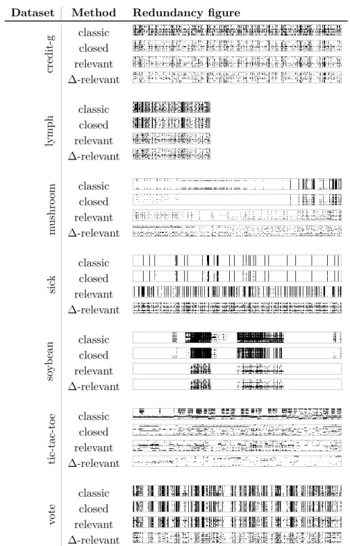
2.10 Redudancy of the top-20 patterns for different algorithms . . . 40

3.1 Vector representation of example cocktails . . . 53

3.2 LSP scalability . . . 67

3.3 Updates per second of MLE . . . 79

3.4 Average pairwise distances of cKPCAand LSP . . . 88

3.5 Execution time of regularcKPCAand using rank-one updates . . . 89

List of Figures

2.1 The pattern space layed out in a lattice . . . 13

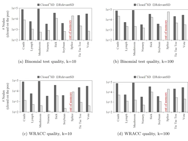
2.2 Number of nodes considered during relevant pattern discovery . . . 25

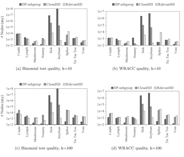
2.3 Number of nodes considered by (non-relevant) pattern mining algorithms 26 2.4 Highly correlated patterns . . . 28

2.5 Condensing redundant patterns creates space in result list . . . 29

2.6 The ∆-dominance relation is not transitive. . . 33

2.7 The dominance graph of Example 2.9. . . 36

2.8 Reduction of ∆-relevant rules found depending on ∆ . . . 38

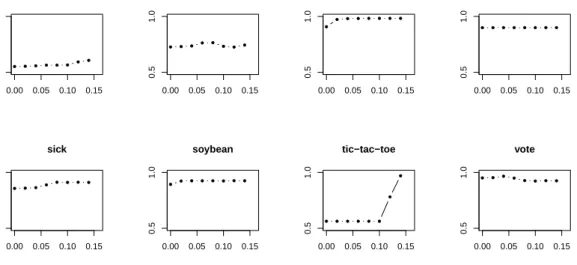
2.9 AUC of the top10 ∆-relevant patterns (Piatetsky-Shapiro quality) . . . 41

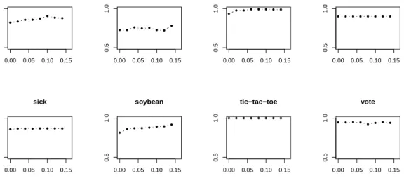
2.10 AUC of the top10 ∆-relevant patterns (Binomial test quality) . . . 42

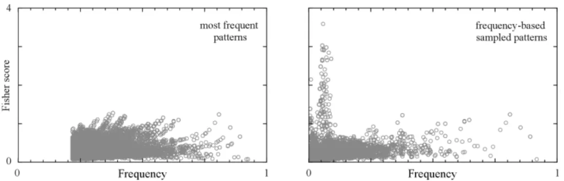
2.11 Primary-tumor dataset: all patterns plotted frequency vs. Fisher score . 43 2.12 Differently drawn patterns, plotted frequency vs. Fisher score . . . 46

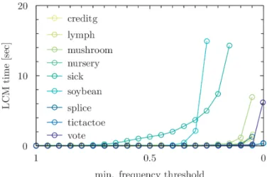
2.13 Execution of LCMwith lowering support threshold . . . 47

2.14 Pattern mining execution time,LCM vs. frequency-based sampling . . . . 48

3.1 Three iterations of projection pursuit . . . 55

3.2 Approximating the distance on a manifold using the knearest neighbors 56 3.3 Highlighting in aPCA embedding via color . . . 59

3.4 Highlighting in aPCA embedding via point size and transparency . . . 59

3.5 Interaction: Filter and re-embed . . . 60

3.6 Interaction: Search and Info-query . . . 61

3.7 Two dimensional projection (shadow) of a cup . . . 62

3.8 Graduate change of an embedding on interaction . . . 64

3.9 LSPscalability rendered updates . . . 66

3.10 LSPscalability calculated updated . . . 66

3.11 LSPscalability speedup . . . 66

3.12 LSPstability experiment . . . 68

3.13 Evolution of mimicking a target embedding via LSP . . . 69

3.14 Development of the rmse for approximating a PCA embedding . . . 70

3.15 Mimicking an embedding depends on the dimensionality of the dataset . 70 3.16 PCAembedding of facial images . . . 71

3.17 Distinguishing between people and poses, using LSP . . . 71

3.18 Zoom into Figure 3.17 . . . 72

3.19 Flexibility of LSP. . . 73

3.21 Spread of cKPCAcompared with LSP . . . 87

3.22 Speedup of cKPCA, using rank-one updates . . . 90

3.23 Flexibility of cKPCA . . . 91

3.24 TheInVistool for interactive embeddings . . . 93

4.1 Plain PCAembedding of the 1000 most frequent patterns . . . 98

4.2 Highlighting ingredients in the PCAembedding of 1000 frequent patterns 99 4.3 Interacting with the embedding of the 1000 most frequent patterns . . . . 99

4.4 Closer inspection of a structure in the embedding of the frequent patterns 100 4.5 Uninformative classic embeddings of 1000 sampled patterns . . . 101

4.6 Revealing structures by interacting with the sampled-pattern-embedding 102 4.7 Highlighting ingredients in the PCAembedding of 1000 subgroups . . . . 103

4.8 Re-embedding of a sub-selection of patterns . . . 103

4.9 Using control points to refine a structure. . . 104

4.10 Inspecting the contents of two of the emerging clusters . . . 104

A.1 Starting up theInVistool. . . 119

A.2 The File menu. . . 120

A.3 The initial view, after the webtender dataset is loaded. . . 121

A.4 The edit menu. . . 121

A.5 Options that can be adjusted in the view menu. . . 123

A.6 A quick reminder of the shortcuts for interaction with the canvas. . . 124

A.7 Queried information on a single data record. . . 125

A.8 A control point. . . 125

A.9 A lasso-selected area and its most influential attribute combinations. . . . 125

A.10 Searching parts of the data record ID’s. . . 126

1. Introduction

“Our information age more often feels like an era of information overload. Excess amounts of information are overwhelming; raw data becomes useful only when we apply methods of deriving insight from it.”

(Scott Murray, Interactive Data Visualization for the Web, 2013)

1.1 Background and Motivation . . . 1

1.2 Contributions . . . 2

1.3 Previously Published Work . . . 5

1.4 Outline . . . 6

1.1. Background and Motivation

Collecting data has become omnipresent. Online retailers collect and evaluate enormous amounts of data to give better product recommendations to their users and thus increase their sales. Companies log and assess information along their processes to optimize their workflows, biologists utilize machine learning techniques on microarrays to discover relations between genes and diseases, and governments collect and analyze communi-cation traces to identify potential threads. Along with the presence of inexpensive and available processing power, storage capacity and communication bandwidth researchers and companies are collecting more and more data with the goal of extracting valuable insights from it. The list of use-cases for discovering knowledge from databases is long and all of them share the hope that the quality of the extracted insights increases with the amount of collected data. Together with the growing processing and storing power, the size of the data collections is steadily increasing; in the amount of assembled data records, as well as the number of attributes that are being monitored.

With this overwhelming amount of data, there is an increasing need for efficient methods that help an analyst to develop an understanding of the data (Chakrabarti et al.,2008). Since there is usually no technique which directly extracts all the relevant insights, the analyst needs to explore the data in order to identify important variables and relations, detect anomalies, coin and test hypotheses and make algorithm and parameter choices.

Exploring the data, can help the analyst to understand the data’s underlying structure, ask the right questions and ultimately uncover the desired insights. In general, extract-ing knowledge from data is an iterative process that involves repetitive modellextract-ing and understanding of it (Shearer,2000) with the ultimate goal to gain previously unknown and potentially useful information (Frawley et al.,1992). To this end exploratory data analysis techniques can help the user to understand the underlying structure and rela-tions of the data. In this thesis two orthogonal approaches were investigated, which both focus on a presentation of the results that is interpretable by a human domain expert. This yields the benefit that an expert of the domain from which the data derives can be empowered to perform knowledge discovery tasks without possessing in-depth machine learning knowledge. The first of the here investigated approaches studies techniques that automatically deliver human-understandable descriptions of interesting partitionings of the dataset to the analyst. The contributions from this part of the thesis to the scientific community are mainly towards finding more concise local pattern descriptions in a more efficient way. The other approach to exploratory data analysis investigates techniques that let the analyst observe all data records of a dataset and their relations at a glance. This part of the thesis studies a novel area of interactive visual data analysis. The idea behind all here introduced approaches is to enable the analyst to browse and navigate a two dimensional Scatter plot projection of the whole dataset in a live-updating and interactive manner. Seeing related data records move in cohesion, while altering the perspective, enables the analyst to understand their connections, coin and test hypothe-ses and the grasp underlying structure of the data itself.

To guide the reader with a consistent example dataset, throughout this thesis a col-lection of cocktail recipes will be used. This colcol-lection is based on 1702 recipes which were retrieved from the website http://webtender.com and it comprises 334 different ingredients. The cocktail dataset is on the one hand complex enough to be interesting and contain non-trivial insights. On the other hand the domain is easily understandable and the reader directly has an intuition for the results. Depending on the task and the utilized algorithms, the cocktail recipe collection is pre-processed differently to form a suitable dataset.

1.2. Contributions

This thesis addresses the human in the loop of data analysis tasks and extends the research on human-understandable knowledge discovery and exploratory data analysis methods by investigating two complementary approaches and their synthesis. The first approach, discussed in Chapter 2, focuses on finding interesting and yet diverse local patterns efficiently. In an exploratory data analysis setting, the discovered patterns can be utilized to guide the analyst’s attention towards interesting sub-populations of the data collection. Employing different pattern mining methods and interestingness measures helps to uncover various aspects within the data. With respect to the pattern mining community, the contributions of this dissertation are the following:

• Section 2.2 presents an efficient algorithm to solve the problem of listing relevant patterns, as introduced by Garriga et al. (2008). It is a variation of an algo-rithm, introduced byBoley and Grosskreutz(2009) to traverse the search space of all closed and positively labeled patterns, following a “shortest-description-length-first” search strategy. The here presented version of the algorithm is designed to exhibit a small memory footprint, by applying an iterative deepening search strat-egy and resulted in a publication at the European Conference on Machine Learning and Principles and Practice of Knowledge Discovery in Databases (Grosskreutz and Paurat,2011).

• A follow-up publication at the SIGKDD Conference on Knowledge Discovery and Data Mining (Grosskreutz et al.,2012), refined the above mentioned relevance to a stricter formulation. The so called ∆-relevance, as introduced in Section 2.3, allows to omit patterns that are redundant to already discovered patterns up to a certain threshold. Employing this pattern mining technique usually leads to a more diverse result set of discovered interesting patterns, which are introduced in Section 2.1.2.

• In contrast to finding a small result set of high-quality patterns, additionally the idea of sampling patterns with a probability proportional to different interest-ingness measures was investigated. This lead to a publication at the SIGKDD Conference on Knowledge Discovery and Data Mining (Boley et al., 2011). The investigated random pattern sampling procedure, as introduced in Section 2.4, can be adjusted to expose different sampling biases that are closely related to different interesting measures.

The second approach to exploratory data analysis that is studied in this dissertation investigates direct interaction with a scatter plot visualization of all data records from a data collection. The main idea behind all techniques, proposed in this work, is to interact with the scatter plot visualization by manually placing individual points of the plot to a desired location. This interaction serves as input to the underlying algorithm, which maps the original data to a two dimensional space that is visualized, to consider the the feedback and re-calculate the mapping accordingly. Interacting with a visualization of all data records and directly receiving response helps the analyst to find interesting sub-populations, craft and check hypotheses and ultimately develop an understanding of the relations among the data records and the underlying structure of the whole dataset. The main contributions to this area of research are the following:

• Section 3.2 introduces a way to interact with and control a (in this case two-dimensional) projection of a dataset, by “grasping and dragging” individual data points within a scatter plot visualization. This technique is not limited to a certain algorithm and can be utilized to express domain knowledge, or to uncover struc-tural properties of the dataset. A first implementation of this interaction method employed theleast squared error projection (LSP) algorithm which solely considers the control points’ data and embedding locations and calculates a linear projection

with the least squared residual error. This lead to a publication at the European Conference on Machine Learning and Principles and Practice of Knowledge Dis-covery in Databases (Paurat and G¨artner,2013) and build the foundation of a tool for interactive visualization (InVis), which is also a part of the contributions of this dissertation.

• A drawback of theLSPmethod is that with no control points placed, the algorithm projects every data record to the origin of the embedding space. To overcome this problem and some other limitations of the LSPmethod, when dealing with sparse data, a probabilistic approach was investigated. The resulting embedding method, discussed in Section 3.3, considers a prior belief about the embedding and regards the placement of the control points as evidence. Section 3.3 also shows that for a certain parameter choice this most likely embedding(MLE) is equivalent to theLSP algorithm. Paurat et al.(2014) discuss the underlying technique in the context of interactive visualizations briefly, as an almost identical mathematical framework was proposed by Iwata et al. (2013).

• An alternative approach to overcome the limitations of LSP and to improve on the flexibility of the underlying embedding algorithm lead to two publications on knowledge based constraint Kernel-PCA (cKPCA). One publication at the NIPS Workshop on Spectral Learning (Paurat et al.,2013b), the other one at the Euro-pean Conference on Machine Learning and Principles and Practice of Knowledge Discovery in Databases (Oglic et al., 2014). cKPCA is an interactive version of a kernel-PCA, as introduced in Section 3.4, that can take several types of constraints into account. These constraints can e.g. be given in the form of desired locations within the embedding of individual points.

The last contribution of this dissertation shows a way of combining pattern discovery and interactive embeddings. Large amounts of patterns tend to overload the analyst with information. For this reason, many pattern mining techniques revolve around the task of finding a small and condensed set of highly interesting and diverse patterns. The combination of pattern discovery and interactive embeddings takes a different approach: • In Chapter 4, a general procedure is introduced, which facilitates interactive em-bedding methods to empower the user to interactively explore and understand large amounts of discovered patterns. Exploring a pattern collection interactively, helps the user to keep an overview on general topics among the patterns and al-lows dive into regions of interest on demand. Following this approach resulted in a publication at the ACM SIGKDD Workshop on Interactive Data Exploration and Analytics (Paurat et al.,2014).

1.3. Previously Published Work

As just stated in Section 1.2 on the contributions of this dissertation, parts of it have already been published in conference and workshop proceedings of the international conference of the Association for Computing Machinery’s Special Interest Group on Knowledge Discovery and Data Mining (ACM SIGKDD), the European Conference on Machine Learning and Principles and Practice of Knowledge Discovery in Databases (ECML PKDD) and the international conference on Neural Information Processing Sys-tems (NIPS). In detail that is:

1. Mario Boley, Claudio Lucchese, Daniel Paurat, and Thomas G¨artner. Direct local pattern sampling by efficient two–step random procedures. InProceedings of the 17th annual ACM SIGKDD Conferences on Knowledge Discovery and Data Mining, 2011

2. Henrik Grosskreutz and Daniel Paurat. Fast and memory–efficient discovery of the top–k relevant subgroups in a reduced candidate space. In Proceedings of the European Conference on Machine Learning and Principles and Practice of Knowledge Discovery in Databases, 2011

3. Henrik Grosskreutz, Daniel Paurat, and Stefan R¨uping. An enhanced relevance criterion for more concise supervised pattern discovery. In Proceedings of the 18th annual ACM SIGKDD Conferences on Knowledge Discovery and Data Mining,

2012

4. Daniel Paurat and Thomas G¨artner. Invis: A tool for interactive visual data analysis. In Proceedings of the European Conference on Machine Learning and Principles and Practice of Knowledge Discovery in Databases, 2013

5. Daniel Paurat, Dino Oglic, and Thomas G¨artner. Supervised PCA for interactive data analysis. InProceedings of the 2nd NIPS Workshop on Spectral Learning, 2013

6. Dino Oglic, Daniel Paurat, and Thomas G¨artner. Interactive knowledge–based kernel pca. In Proceedings of the European Conference on Machine Learning and Principles and Practice of Knowledge Discovery in Databases, 2014

7. Daniel Paurat, Roman Garnett, and Thomas G¨artner. Interactive exploration of larger pattern collections: A case study on a cocktail dataset. In Proceedings of the 2nd ACM SIGKDD Workshop on Interactive Data Exploration and Analytics,

1.4. Outline

This section connects the chapters and sections by providing an outline through the thesis. Chapter 2 tackles different local pattern mining techniques that can be useful to an analyst in an exploratory data mining setting. Starting with the preliminaries and introducing the formal notation the Sections 2.2, 2.3 and 2.4 deal with efficient listing and sampling of local patterns. All of these techniques automatically find interesting descriptions of partitionings of the dataset, guiding the analysts attention towards sta-tistically outstanding sub-populations of the data distribution. Sections 2.2 and 2.3 investigate relevant and ∆-relevant pattern mining methods. These techniques aim at efficiently listing the top non-redundant, concise and interesting subgroup descriptions of a labeled transactional database. Section 2.4 introduces a fast way to sample local patterns according to different interestingness measures. The chapter then concludes with a summary and discussion of the techniques.

Having investigated techniques that automatically find and deliver interesting aspects of the dataset, Chapter 3 changes the focus and studies methods that enable the analyst to observe and interact with a projection of the whole dataset. Being able to observe all data records and their relations at once and to directly interact with them, lets the analyst study the dataset “from a bird’s eyes perspective” and discover interesting aspects on his own. This way the analyst can decide for himself which partitionings are of interest. The chapter starts again by introducing the preliminaries to these techniques and then continues to introduce three different algorithms that project the data into a lower dimensional space and allow the analyst to directly alter the projection. For the purpose of interactive visual analysis this lower dimensional space is the 2d plane. Here, the analyst can actively browse the whole dataset in a visual way, see some of the relations among the data records and understand the underlying structure of the dataset. Navigating the projection is done by relocating individual data records within the visualization in a “drag and drop” like manner. Selecting and relocating such a “control point” triggers the underlying embedding algorithm to consider the analysts feedback and shift the projection angle accordingly. This work introduces three different interactive embedding techniques that utilize the placement of control points to alter the projection of the data. Section 3.2 introduces a straight forward approach to interact with a projection via control points. From the here presented methods this is the fastest and most scalable algorithm. However, the approach is limited in several ways. For instance, with no control points given, the embedding collapses to the origin. Another limitation comes when dealing with sparse data. In this case, poorly chosen, or too few, control points can lead to a degenerated embedding that doesn’t reveal any interesting aspect of the data. To overcome some of the limitations, in Section 3.3 a probabilistic version of an interactive embedding algorithm presented. Without any control points placed, it is able to start with a prior belief about a “good” projection of the data. Note that a similar idea has been published independently byIwata et al.(2013). Although it does not focus on the interaction with the embedding, the underlying mathematics are largely alike. Section 3.4 studies an alternative approach to overcome the limitations

of the initial approach to interact with the embedded data. It presents an interactive version of a kernel PCA. This way, the embedding is not limited to linear projections any more, the initialization problem is solved and sparse datasets do not degenerate, as the variance among the data records is naturally taken into account. However, these benefits come at the price of computational complexity. The chapter concludes again with a summary and discussion.

The ideas and methods, presented in the Chapters 2 and 3 represent two very different approaches to exploratory data analysis and on how to find, study and understand the driving aspects of a dataset. Chapter 4 presents a natural way of combining these approaches, by interactively and visually analysing large pattern collections. To do so, the mined patterns have to be represented as vectors.

The final Chapter 5 concludes with a general discussion on this thesis, open issues and further research areas that might possibly emerge from this work.

2. Local Pattern Discovery

2.1 Preliminaries . . . 10 2.2 Relevant Patterns . . . 16 2.3 ∆-Relevant Patterns . . . 28 2.4 Sampling Interesting Patterns . . . 42 2.5 Summary and Discussion . . . 48

In an exploratory data analysis setting, the analyst tries to find interesting aspects of the data. This can be done, for instance, by studying and understanding the underlying distribution from which the data derives. Pattern mining can be of help here, as it auto-matically finds human interpretable descriptions of interesting partitionings of the data. In an exploratory setting, these patterns can be used to guide the analyst’s attention towards interesting aspects of the dataset. This chapter investigates how to efficiently find interesting and yet diverse local patterns. To this end, two fundamentally different pattern mining approaches are studied. The first one considers the space of all possible patterns that are defined on a dataset and reports a small set of highly interesting, yet non-redundant, ones. One way of avoiding redundancy in a pattern discovery scenario, is to focus on the so called relevant patterns. As a contribution, this work proposes a novel algorithm for listing the top relevant patterns. The algorithm is faster and possesses a smaller memory footprint than it’s competitors. In addition, the notion of relevance is re-considered to allow for some slack, which in terms yield a less redundant and more condensed result set. Another pattern mining approach that avoids redundancy in a natural way, is to randomly sample them. This work introduces a sampling procedure that can be adjusted to draw random patterns with a probability proportional to differ-ent interestingness measures. This way, the analyst can explore patterns with a certain bias towards an interestingness measure, but is not strictly bound to the “top” ones. In an exploratory setting, this leaves room to discover patterns that are highly attractive to the analyst, but are not considered interesting in terms of the measure.

2.1. Preliminaries

The following section gives an introduction to the notation of pattern mining. It provides the definition of a pattern that is used throughout this work, introduces basic concepts and notions like, e.g., extention and support, the true- and false positives of a pattern for a labeled dataset, and presents several measures of interest for a given pattern. 2.1.1. Patterns

For the task of pattern mining, we assume a databaseD of m data records, d₁, . . . , dm,

with each data record being described by a set of n binary attributes, or features, ˆa₁ˆdi, . . . , anˆdi > ˜0,1n. A pattern p is a subset of the attribute set, i.e.

p b ˜a₁, . . . , an, with each single ai of the pattern being referred to as item. For a given database D, a data record d satisfies a pattern p if aˆd 1 for all a > p, that

is, patterns are interpreted conjunctively. The cardinality of a pattern SpS denotes the

number of contained items, meaning the number of attributes a for which aˆd 1.

Sometimes also the notationai1&. . .&aik is used instead of˜ai1, . . . , aik, omitting the

items for whichaˆd 0. In addition, this work also refers to a pattern as a subgroup descriptionorsubgroup. This comes due to the fact that parts of the here presented

research were done in the specific pattern mining area of subgroup discovery. Subgroup descriptions are “regular” patterns in terms of their representation. The difference is that in order to measure the interestingness of a subgroup, an additional feature, the label, is considered. Hence, subgroup discovery algorithms explicitly consider labeled datasets and perform the task of finding frequent patterns that exhibit an unusual label distribution in comparison to the overall label distribution.

The expression D p, also referred to as the extention of p, describes the set of data

records d> D of a database D that satisfy the pattern p. The support of p, denoted

by suppˆD, p or short suppˆp, is the cardinality of the set of data records that are

described by D p. Considering the cocktail dataset, a pattern could for instance be Vodka & Orange juice. It describes the extention of all cocktails which contain Vodka

and Orange juice at the same time. The Table 2.1 below shows an excerpt of five

cocktails represented as transactions from our exemplary cocktail database.

Id Name Itemset

1 Caipirinha Cacha¸ca & Lime & Sugar

2 Mojito Light rum & Lime & Mint & Soda water & Sugar

3 Pi˜na Colada Coconut milk & Light rum & Pineapple

4 Screwdriver Vodka & Orange juice

5 Tequila Sunrise Grenadine & Orange juice & Tequila

Table 2.1.: An itemset representation of five well known cocktails. The listed ingredients indicate their presence in the cocktail.

Additionally, the data records can be associated with a label. For the sake of simplicity, here only binary labels are considered, though in practice not all pattern mining meth-ods are restricted to that. Formally, the label is a special attribute classˆd that has

the range ˜`,\.

For such a binary labeled dataset the true positives (T P) and the false positives

(F P) of a pattern pcan be defined, with respect to the databaseD, as TPˆD, p ˜d> D p Sclassˆd ` and FPˆD, p ˜d> D p Sclassˆd \.

The cardinalities of the sets STPˆD, pS and SFPˆD, pS are denoted by suppˆp and

respectively supp_ˆp.

To stay in the previously given example of the cocktail dataset, the pattern Vodka

& Orange juice describes the extention of all cocktails in our database that contain

both ingredients Vodka and Orange juice at the same time. In our dataset there are

95 cocktails which support this pattern. Considering a label that indicates whether a cocktail is creamy or not, only 5 out of the 95 cocktails are labeled as creamy. These five data records are the true positives of the pattern, the other 90 form the false positives. 2.1.2. Interestingness of a Pattern

The interestingness of a pattern p in the context of a database D is measured by a quality function qˆD, p that assigns a real-valued quality top. As patterns can be of

interest for different reasons, there are diverse measures to determine the interestingness of a pattern. One common interestingness measure is the frequency of a pattern. It is defined as the share of data records that are supported by the pattern over the amount of all data records

freqˆD, p suppˆD, p

SDS .

Another prominent measure that does also not consider labels is the so called liftof a

pattern. It compares the observed support of a pattern to its expected support if all the attributes were statistically independent. For instance, when considering the cocktail dataset, 452 out of the 1702 cocktails contain Vodka and 249 Orange juice. That is,

26.5% of the cocktails contain Vodka and 14.6% Orange juice. If we assume that the

occurrence of these ingredients is independent, we would expect to observe that 3.8% of all cocktails contain both ingredients at the same time. However, in the data we observe 5.6% (95 cocktails) containing both ingredients. As this is almost 1.5 times our expected value, the pattern Vodka& Orange juice is lift-wise considered as interesting.

More formally, the lift of the pattern pon the datasetD is defined as

liftˆD, p freqˆD, p Lpi>pfreqˆD, pi

Other prominent measures of interest additionally consider labels that are assigned to the data records. To see how this can be of value, let us consider a label for the cocktail dataset that indicates whether a cocktail is creamy, or not. For our previous example patternVodka & Orange juice, only 5 out of 95 cocktails which supported the pattern

were creamy. Compared to the overall distribution, where 368 out of 1702 cocktails are labeled as creamy, the pattern under-represents the creamy cocktails. The shift of how much the label distribution of a pattern’s extention deviates from the overall label distribution can be utilized as an interestingness measure. However, note that considering solely the ratio betweenS ` SandS \ Scan be very sensitive to the amount of supporting data records. If, e.g., another patternpœ would only be supported by a single

data record that also happens to be labeled as creamy, the ratio would be 1 out of 1. Although the ratio indicates a highly interesting pattern, the extention that the pattern describes would be much too small to be interesting to the analyst. To account for this drawback, the ratio is usually weighted by a function of the frequency of the pattern. This yields a quality measure which promotes patterns that expose a larger extention and have an unusual label distribution. Some of the most common quality functions for binary labeled data that capture this are of the form

qˆD, p SD pSα ŒSTPˆD, pS

SD pS

STPˆD,gS

SDS ‘, (2.1)

where α is a constant such that 0 @αB1, and TPˆD,g simply denotes the set of all

positively labeled data records in the dataset. The family of quality functions char-acterized by this equation includes some of the most popular quality functions: for

a 1, it is order equivalent to the Piatetsky-Shapiro quality function (Kl¨osgen, 1996)

and the weighted relative accuracy (WRACC) (Lavraˇc et al.,2004), while fora 0.5 it

corresponds to the binomial test quality function (Kl¨osgen,1996). 2.1.3. Listing Patterns

This section gives a brief introduction to the algorithmic approach of enumerating inter-esting patterns in an efficient way. Many pattern mining techniques find the interinter-esting patterns by traversing the space of all possible patterns over the given attributes in a systematic way. Hereby the patterns are generated one after another and the quality of the pattern is measured (and reported).

Traversing the Pattern Space

Many pattern mining algorithms consider the set of all possible patterns over a set of attributes, ordered in a general to specific manner, as search space and traverse it in order to find the interesting patterns. Figure 2.1 displays this search space for a dataset over the three attributes a₁, a₂ and a₃. Here the patterns are connected by an edge, if

they are in a super-/subset relation and differ by only one item. The patterns in this lattice are arrange in the so called general to specific order. As each item of a pattern

constitutes a constraints, the empty set, a pattern with no items, is the most general one. It does not exhibit any constraint and thus is supported by all data records of the data set. The opposite constitutes the set of all items. Usually there are no, or only very few, data records that satisfy all possible constraints and contribute to the support set of the most specific pattern. Note that for any amount of attributes the general to specific ordered search space always starts and ends in a single node, the empty set and the set of all attributes.

Figure 2.1.: All patterns that can be formed from the attributes a₁, a₂ and a₃. The

connections denote the super-/sub-set relation between the patterns. Starting from the empty pattern, with each step down in the lattice, the patterns become more specific. Traversing this pattern-lattice in a systematic way is the basis for a whole family of pattern mining algorithms. Most of them can be seen as an instance, or a refinement of the MIDOSalgorithm (Wrobel,1997). The difference among pattern mining algorithms can often be found in the traversal strategy. Depending on the objective of the algo-rithm, they usually start at one of the single-node endpoints and perform a breadth-, or a depth-first-search on the graph. In addition, there are several methods that let the al-gorithms terminate faster, or have a smaller memory footprint. One of these techniques, for instance, is that the algorithms avoid multiple visits of the same node. More com-plicated refinements involve an iterative deepening traversal strategy, or the application of a heuristic in order to perform a greedy beam-search. Another common technique which will be introduced in the following section is the so called pruning. In a scenario where only a fix amount of the highest quality patterns are desired, pruning can help to drastically reduce the runtime of an algorithm by excluding vast parts of the search space from the search.

Frequency and Optimistic Estimator Pruning

Consider again our cocktail dataset. In this dataset, there are 334 different ingredients and each of them may occur in a pattern, or not. This means that there are 2334 different patterns possible, a number with hundred and one digits. Usually it is not feasible to test all of these patterns exhaustively for their interestingness, however, there are ways to deal with this massive amount of patterns. Many interestingness measures are anti-monotone towards specializations of a pattern. This means that

specializing a pattern can only lower, of retain the interestingness. As a consequence for these interestingness measures, any specialization of a non-interesting pattern is also not interesting. State-of-the-art top-k pattern mining algorithm do not traverse the

whole space of candidate patterns explicitly, but apply pruning to reduce the number of patterns effectively visited (Atzm¨uller and Lemmerich, 2009; Grosskreutz et al., 2008; Nijssen et al.,2009). The use of such techniques results in a dramatic reduction of the execution time and is an indispensable tool for fast exhaustive subgroup discovery and pattern mining algorithms in general (Atzm¨uller and Lemmerich, 2009; Grosskreutz et al.,2008;Morishita and Sese,2000).

Consider a scenario, where the analyst is only interested in the top-k most frequent

patterns of a dataset. In this case, not all patterns have to be tested for their fre-quency. The support, or frequency, of a pattern is a quality measure that is in an anti-monotone relation to the description length of the pattern. This can easily be understood, if each item of a pattern is interpreted as a constraint on the data records that support the pattern. The more constraints a pattern exhibits, the less data records are able to fulfill all of them. This means that specializing a pattern, by augmenting it with a new item, can only retain or lower the original support, but never increase it (¦ pœ cp suppˆD, pœ BsuppˆD, p). Hence, if a pattern does not exhibit a certain

minimum support, none of its specializations will. When searching for the k most

frequent patterns, the quality of thekth best pattern found so far can be utilized as a

minimum frequency threshold. While the algorithm finds better patterns, this threshold increases dynamically and the part of the search space with patterns that can potentially be among thekbest ones shrinks. By dynamically increasing this threshold, the pattern

space left to explore for the algorithm can be pruned Combined with a quality-bound on all specializations of patterns, a dynamically increasing threshold allows to ignore large parts of the search space, as it is guaranteed that all specializations of already ruled out patterns do not possess the desired minimum support.

A closely related concept is that of anoptimistic estimate(Grosskreutz et al.,2008).

An optimistic estimator is a function that provides a bound on the quality of a pattern and of all its specializations. Formally, an optimistic estimator for a quality measure q

is a function oe that maps a database D and a pattern p to a real value such that for

all D,p and specializations pœcp, it holds thatoeˆD, p CqˆD, pœ. Note that pattern

mining algorithms, which traverse the lattice of all patterns, scale exponentially with the amount of attributes. Utilizing an optimistic estimate pruning technique remedies this effect in practice to a certain extend, as it improves the expected runtime performance drastically (Grosskreutz et al.,2008;Morishita and Sese,2000).

Reporting only thekbest patterns also has the benefit that the resulting set of interesting

patterns has a convenient size for a human analyst. However, thek reported patterns

not only contain few highly interesting patterns, but also diverse ones. A common way to promote diversity in the result set is to avoid redundancy among the patterns via a closure system.

2.1.4. Avoiding Redundancy via a Closure System

A common mathematical framework that pattern mining methods employ to avoid re-dundancy among the reported patterns is that of a closure operator. A closure

oper-ator Γ on a set S is a function Γ PˆS PˆS from the power set ofS into the power set ofS that has to satisfy the following three properties for any two sets s, sœ> PˆS:

1. sbÈs (extensivity)

2. sbsœΓˆs bÈsœ (monotonicity)

3. Ès ÈÈs(idempotence)

The closed sets are the fixpoints of a closure operator on a dataset (Pasquier et al., 1999). Closed pattern mining algorithms find the (usually top-k) closed patterns of a

dataset. The above definition allows for different realizations of the closure operator. One that has a broad application in pattern mining considers patterns of maximal description length in their support equivalence class as closed. Note, that a closure may have different generator sets, but that there is only one unique set of maximal description length.1 _This instantiation of the closure operator will be used throughout this work. This means that a pattern p is closed if and only if there is no pœ a p that is supported by the same

data records. Using this concept of the closure operator, classic closed pattern mining algorithms report only the (unique) pattern of maximal description length for a support equivalence class. An example of this closure operator is illustrated on the following dataset: Id a₁ a₂ a₃ a₄ 1 1 1 1 1 2 1 1 1 0 3 1 1 1 0 4 1 1 0 0 5 1 1 0 0

Table 2.2.: A dataset to illustrate closed sets.

1 _{If two patternsp}

1andp2 possess exactly the same extention, thenp18p2also possesses this extention. (For illustration, have a look at the patterns ˜a1and ˜a2in Table 2.2.) The union of all patterns of a support equivalence class P8 is of maximal length. There is also only one pattern of maximal description length, because if there was another different patternPœ of the same support equivalence class with the same (maximal) length,Pœ would have been part ofP8 in the first place. AsP8 is the union of all patterns of that support equivalence class andPœxP₈,Pœ`P₈and henceSP₈S A SPœS.

Consider the patterns ˜a₁, ˜a₂ and ˜a₁,a₂. All of them are supported by exactly

the same data records with the Ids ˜1,2,3,4,5, hence, they are in the same support equivalence class. For these three patterns the one with the longest description length,

the pattern ˜a₁,a₂, is chosen as their representative. The tile that it spans in the

dataset is highlighted in Table 2.2 with a dark blue outline. The other closed patterns of this example dataset are the pattern˜a₁,a₂,a₃and the pattern˜a₁,a₂,a₃,a₄.

Any of the 16 possible patterns over the attributesa₁ toa₄ belongs to one of the support

equivalence classes, described by those four patterns.

Why is avoiding redundancy among the reported patterns interesting? As stated earlier, there is a huge space of candidate patterns that are potentially interesting to the analyst. Even after eliminating all obviously not interesting patterns, the remaining collection is usually still vast. As a human analyst is only capable of reviewing a small amount of output patterns, most pattern mining algorithms try to deliver a compact set of high quality patterns. For this small collection of patterns it is of great value, if the contained patterns represent different concepts of the underlying distribution. A good way to promote diversity is to discard patterns with redundant information.

There are many fast implementations of algorithms that find the frequent closed patterns of a dataset. Of particular interest to us areIMRandLCM(Boley and Grosskreutz,2009;

Uno et al.,2004), as they essentially perform depth first and breadth first search on the space of the closed patterns. It is also notable that implementation ofLCMbyUno et al. (2004) was the winner of the FIMI contest (Bayardo et al.,2004) and is known among the pattern mining community for it’s fast execution.

2.2. Relevant Patterns

The theory of relevance (Lavraˇc and Gamberger, 2005; Lavraˇc et al., 1999) aims at eliminating irrelevant patterns, respectively subgroups. Similar to the closed patterns, this remedies some of the redundancy among the finally reported patterns.

2.2.1. A Definition of Relevance

In order to be able to apply the theory of relevance to pattern mining approaches, the patterns have to be closed and the data records have to possess a binary label. Given this, a closed patternp_irr is consideredirrelevant if it is dominated(orcovered) by

another closed pattern p. More formal, a closed pattern p_irr is considered irrelevant if

and only if a different closed patternp exists in databaseD with

i) TPˆD,p_irr bTPˆD,pand (2.2)

All patterns that are not dominated are considered relevant. Applying the theory of

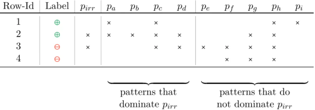
relevance to pattern mining yields a set of finally reported patterns that are all closed and relevant. This means that for each of the not reported patterns there is a dominating relevant pattern in the result which is potentially of more value. The following Table 2.3 shows an example of the domination relation for the patternpirr on a toy dataset of only four labeled data records.

Row-Id Label pirr pa pb pc pd pe pf pg ph pi

1 `

2 `

3 \

4 \

´¹¹¹¹¹¹¹¹¹¹¹¹¹¹¹¹¹¹¹¹¹¹¹¹¹¹¹¹¹¹¹¹¹¹¹¹¹¹¹¹¹¹¹¹¹¹¹¹¹¹¹¹¹¹¹¸¹¹¹¹¹¹¹¹¹¹¹¹¹¹¹¹¹¹¹¹¹¹¹¹¹¹¹¹¹¹¹¹¹¹¹¹¹¹¹¹¹¹¹¹¹¹¹¹¹¹¹¹¹¹¹¹¶ ´¹¹¹¹¹¹¹¹¹¹¹¹¹¹¹¹¹¹¹¹¹¹¹¹¹¹¹¹¹¹¹¹¹¹¹¹¹¹¹¹¹¹¹¹¹¹¹¹¹¹¹¹¹¹¹¹¹¹¹¹¹¹¹¹¹¹¹¹¹¹¹¹¹¹¹¹¹¹¹¸¹¹¹¹¹¹¹¹¹¹¹¹¹¹¹¹¹¹¹¹¹¹¹¹¹¹¹¹¹¹¹¹¹¹¹¹¹¹¹¹¹¹¹¹¹¹¹¹¹¹¹¹¹¹¹¹¹¹¹¹¹¹¹¹¹¹¹¹¹¹¹¹¹¹¹¹¹¹¹¶ patterns that patterns that do dominate pirr not dominate pirr

Table 2.3.: A dataset of four labeled data records that exemplifies the dominance relation. The -symbol indicates that the pattern supports the data record with the according Row-Id.

Here, the -symbol indicates that a data record, identified by its Row-Id, supports a pattern. In the sense of the above defined dominance relation the pattern pirr is dominated by the patterns pa, pb, pc and pd. All of these patterns cover all positively labeled instances of pirr (and possibly more), while covering at maximum all negatively labeled instances ofpirr. Note that it is possible for two patterns to dominate each other (see pirr and pd), however only in the case that they have an identical extention. In this case, they share a common unique representative, the earlier introduced closure (See Section 2.1.4). On the other hand, the patternspe,pf,pg,ph andpido not dominate the pattern pirr. Some of these patterns do not cover all of the positively labeled instances that support pirr, others cover a superset of the negatively labeled data records. Note that all patterns pa. . . ph have an overlap in their support set with the one of pirr. The patternspi andpirr, however, have no overlap in their support sets. Herepi can be seen as a representative for all patterns that possess this property. Meaning, thatpi and pirr cannot dominate each other, as they are set-wise not comparable.

2.2.2. A Reformulation of Relevance

As shown by Garriga et al. (2008), the notation of relevance, as stated in equation 2.2, can be restated by using the closure operator over a set of attributes A, only on the

positively labeled data records

Γ _{is a closure operator, as introduced in Section 2.1.4, meaning that it is a function} defined on the power-set of attributes Pˆ˜a₁, . . . , an such that for all patternsp, pœ >

Pˆ˜a₁, . . . , an, (i) pb Èp (extensivity), (ii) p b pœ Èp bÈpœ (monotonicity),

and (iii) Èp ÈÈp(idempotence) holds. The fixpoints of Γ, i.e. the patterns for

which p Èp, will further on be referred to as the closed-on-the-positives. The

main result of Garriga’s research for mining the relevant patterns in an efficient way is the following:

Proposition 1 The space of relevant patterns consists of all patterns p_rel satisfying the following:

(i) p_rel is closed-on-the-positives, and

(ii) there is no generalization pøp_relthat is closed-on-the-positives such thatSFPˆD,pS SFPˆD,prelS.

This connection between relevancy and closure operators is particularly interesting be-cause closure operators have extensively been studied in the area of closed pattern mining (Boley and Grosskreutz, 2009; Kl¨osgen, 1996; Pasquier et al., 1999; Uno et al., 2004). However, unlike here, traditional closed pattern mining algorithms do not account for the label of the data.

2.2.3. Listing all Relevant Patterns

The publication ofGarriga et al. (2008) is the first that proposes an approach to solve the relevant pattern discovery task. Making use of Proposition 1,Garriga et al. (2008) have proposed a simple two-step approach to find the relevant patterns:

1. Find and store all closed-on-the-positives

2. Remove all dominated closed-on-the-positives using Proposition 1

In the following, this subgroup discovery approach will be referred to asClosedSD. The search space considered by this algorithm — the closed-on-the-positives — is a subset of all closed patterns, thus it operates on a potentially exponentially smaller candidate space than all earlier approaches. The downside is that it does not account for optimistic estimate pruning, and that it has very high memory requirements, as the whole set of closed-on-the-positives has to be stored.

2.2.4. Efficient Listing of the Top-kRelevant Patterns

In the following, an algorithm is derived that possesses a memory-efficient way to test the relevance of a newly visited pattern while traversing the pattern space. For many datasets it is infeasible to store all closed-on-the-positive patterns in memory and then apply Proposition 1 to test for relevance. Instead, the following observation leads to a solution:

Proposition 2 LetDbe a dataset, qˆ be a quality function of the form of Equation 2.1 and θ some real value. Then, the relevance of any closed-on-the-positive p withqˆp Cθ can be computed from the set of all generalizations of p with qˆp Cθ:

G‡ ˜p_genøpSp_gen is relevant in D andqˆD,pgen Cθ

In particular, p is irrelevant if and only if there is a relevant pattern p_gen in G‡ with the same negative support.2

To prove the correctness of Proposition 2, we first present two lemmas:

Lemma 3 If a closed-on-the-positive p_irr is irrelevant, i.e. if there is a generalization pøp_irr closed on the positives with the same negative support as p_irr, then there is also at least one relevant generalization p_reløp_irr with the same negative support.

Proof Let N be the set of all closed-on-the-positives generalizations of p_irr with the

same negative support as p. There must be at least one p_rel inN such that none of the

patterns in N is a generalization of p_rel. From Proposition 1, we can conclude thatp_rel

must be relevant and dominates p_irr. _j

Lemma 4 If a relevant pattern p_reldominates another pattern p_irr, then p_relhas higher quality than p_irr.

Proof As a pattern can only be dominated by its generalizations and because

sup-port is antimonotonic, we have that SD prelS C SD pirrS. Thus, to show that p_rel

has higher quality, it is sufficient to show STPˆD,p_relS~_SDp

relS A STPˆD,pirrS~SDpirrS. Be-cause p_rel has to be a generalization of p_irr and because of the anti-monotonicity

property, we can conclude that p_rel and p_irr have the same number of false

posi-tives; let F denote this number. Using F, we can restate the above inequality as

STPˆD,prelS~ˆSTP_ˆD,p_relS F_ A STPˆD,pirrS~ˆSTP_ˆD,p_irrS F. All that remains to show is thus that STPˆD,prelS A STPˆD,pirrS. By definition of relevance, STPˆD,prelS C STPˆD,p_irrS, and because p_rel and p_irr are different and closed on the positives, the

inequality must be strict, which completes the proof. j

Based upon these lemmas, it is straightforward to prove Proposition 2:

Proof We first show that if p is irrelevant, then there is a generalization in G‡ with

the same negative support. From Lemma 3 we know that ifp is irrelevant, then there is

at least one relevant generalization of p with same negative support dominating p. Let p_genbe such a generalization. Lemma 4 implies thatqˆD,pgen CqˆD,p Cθ, hencep_gen

is a member of the set G‡.

It remains to show that ifp is relevant, then there is no generalization in G‡ with same

negative support. This follows directly from Proposition 1. j

2 _{Only the support is needed, asp}

Proposition 2 tells us that we can perform the relevance check based only on the top-k

relevant patterns visited so far: Applying an iterative deepening traversal strategy of the space of all patterns in a general to specific order ensures that a patternp is only

visited, once all of it’s generalizations have been visited first; so if the quality of the newly visited patternpexceeds that of thekth-best pattern visited so far, then the set of

the bestkrelevant patterns visited includes all generalizations ofp with higher quality;

hence, we can check the relevance of p. On the other hand, if the quality of p is lower

than that of thekth-best pattern visited, then we don’t care about its relevance anyways.

This leads us to the relevant subgroup discovery Algorithm 1, further on referred to as RelevantSD. The main program is responsible for the iterative deepening. The actual work is done in the procedure findSubgroupsWithDepthLimit, which traverses the space of the closed-on-the-positives in a depth-first fashion using astackdata structure. Thereby,

it ignores found (closed-on-the-positive) patterns that are longer than the length limit, and avoids multiple visits of the same node using a standard technique like the prefix-preserving property test (Uno et al., 2004). Moreover, the function applies standard

optimistic estimate pruning and dynamic quality threshold adjustment. The relevance check is done in line 6, relying on Proposition 2.

Let us now turn to the complexity of the algorithm and analyse it. To do so, let n

denote the number of attributes in the dataset and m the number of records. Given

that the maximum recursion depth isn, the maximum size of the result queue isk, and

every pattern has length Oˆn, the algorithm has to store at maximum n patterns of

lengthn, plus thek results (also of length n). This results in a memory complexity for

theRelevantSDalgorithm in the order ofOˆn2kn.

For the runtime complexity, the following observations have to be considered and put together: For every node visited, the algorithm computes the quality, tests for rele-vance and considers at most n augmentations. The quality computation can be done

in Oˆnm, while the relevance check can be done in Oˆkn. The computation of the

successors in Line 5 involves the execution of n closure computations, each in Oˆnm,

which amounts toOˆn2m. Altogether, the cost-per-node is thusOˆn2mkn. Finally,

the number of nodes considered is obviously bounded byOˆSCpSn, whereCpis the set of

closed-on-the-positives and the factor nis caused by the iterative deepening approach.

So all put together, theRelevantSDalgorithm has a time complexity ofOˆSCpS n3mn2k.

Table 2.4 compares the runtime and space complexity of the RelevantSD algorithm with that of ClosedSD, classical depth first search subgroup discovery with pruning (DP-subgroup) and closed subgroup discovery algorithms (ClosedSD). Although these algorithms solve a different and simpler task, it is interesting to observe they do not have lower complexities. The expressionS used in the table denotes set of all subgroup descriptions, whileC denote the set of closed subgroups.

Algorithm 1 Iterative Deepening Top-k RelevantSD

Input : An integerk, a database D over attributes˜f₁;...;fn,

a quality function qˆwith an optimistic estimatoroeˆ

Output : The top-k relevant subgroups main:

1. let result = queue of maximum capacity k(initially empty)

2. let θ= 0

3. forlimit = 1 to n do

4. findSubgroupsWithDepthLimit(result,limit,θ)

5. end for

6. return result

procedure findSubgroupsWithDepthLimit(result,limit,θ):

1. let stack = new stack initialized withg as initial pattern

2. while stack not emptydo

3. let next = pop from stack

4. if SnextS Blimit and oe(next) Aθthen

5. add all direct specializations ofnext tostack (avoiding multiple visits)

6. if q(next) A θ and is not dominated by any pœ>resultthen

7. add next toresult

8. updateθ tominˆ ˜qˆp S ¦p>result 

9. end if

10. end if

11. end while

Let us consider some of the properties of these algorithms in more detail, starting with the memory complexity: Except for ClosedSD, all approaches can employ depth-first-search and thus have moderate memory requirements. ClosedSD, on the other hand, has to collect all closed-on-the-positives, each of which has a description of length n.

Please note that no pruning is applied, meaning that nSCpSis not a loose upper bound

for number of nodes stored in memory, but the exact number — which is why the Θ-notation in Table 2.4 is used. As the number of closed-on-the-positives can be expo-nential inn, this approach can quickly become infeasible.

As for the runtime, let us compare the complexity of RelevantSD with that of classic, and respectively closed subgroup discovery algorithms. Probably the most important difference is that the algorithms operate on different spaces. While the time complexity of RelevantSDis higher by a linear factor (resp. quadratic, compared to classic subgroup discovery), the search space, i.e. the closed-on-the-positives Cp, can be exponentially smaller than the one considered by the other approaches (i.e. C, respectively its superset S). The exponential difference in the size of the search space can easily be seen for

Algorithm Memory Runtime Pruning

DP-subgroup Oˆn2kn OˆSSS nm yes

ClosedSD Oˆn2kn OˆSCS n2m yes

ClosedSD ȈnSCpS ȈSCpS n2m no

RelevantSD Oˆn2kn OˆSCpS n3mn2k yes

Table 2.4.: Runtime and memory complexity of different pattern discovery approaches, compared to the here proposed RelevantSDalgorithm.

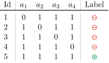
datasets that are constructed as follows: We define a binary datasetDn d₁, . . . , dn, dn1 withn1 data records overnattributesa₁, . . . , an and a label. The firstndata records are constructed as

ajˆdi ¢¨¨¦¨¨ ¤

0, ifi j

1, otherwise and Labelˆdi \

The dataset is then augmented with an additional entry dn1, which contains solely 1-entries and a positive class label ˆ1, . . . ,1,`. In this family of datasets, every pattern

is closed. The total number of closed patterns is thus 2n_{, while there is only one} closed-on-the-positives, namely˜a₁. . . an. The below Table 2.5 illustrates such a construction

for four attributes.

Id a₁ a₂ a₃ a₄ Label 1 0 1 1 1 \ 2 1 0 1 1 \ 3 1 1 0 1 \ 4 1 1 1 0 \ 5 1 1 1 1 `

Table 2.5.: A dataset with exponentially fewer closed-on-the-positive patterns than regular-closed ones.

Finally, compared to ClosedSD, we see that in worst-case the iterative deepening ap-proach causes an additional factor of n (the second term involving k is not much of a

problem, as in practice k is relatively small). For large datasets, this disadvantage is

however outweighed by the reduction of the memory footprint, which allowsRelevantSD to work datasets that cannot be processed by ClosedSD. Moreover, as the following section will show, in practice this worst-case seldom happens: on real datasets, due to the use of pruning,RelevantSD is mostly able to outperform ClosedSD.