Mantesi, Eirini and Hopfe, Christina J. and Cook, Malcolm J. and Glass,
Jacqueline and Strachan, Paul (2018) The modelling gap : quantifying
the discrepancy in the representation of thermal mass in building
simulation. Building and Environment, 131. pp. 74-98. ISSN 0360-1323 ,
http://dx.doi.org/10.1016/j.buildenv.2017.12.017
This version is available at https://strathprints.strath.ac.uk/64551/
Strathprints
is designed to allow users to access the research output of the University of
Strathclyde. Unless otherwise explicitly stated on the manuscript, Copyright © and Moral Rights
for the papers on this site are retained by the individual authors and/or other copyright owners.
Please check the manuscript for details of any other licences that may have been applied. You
may not engage in further distribution of the material for any profitmaking activities or any
commercial gain. You may freely distribute both the url (
https://strathprints.strath.ac.uk/
) and the
content of this paper for research or private study, educational, or not-for-profit purposes without
prior permission or charge.
Any correspondence concerning this service should be sent to the Strathprints administrator:
[email protected]
The Strathprints institutional repository (https://strathprints.strath.ac.uk) is a digital archive of University of Strathclyde research outputs. It has been developed to disseminate open access research outputs, expose data about those outputs, and enable the
Contents lists available atScienceDirect
Building and Environment
journal homepage:www.elsevier.com/locate/buildenvThe modelling gap: Quantifying the discrepancy in the representation of
thermal mass in building simulation
Eirini Mantesi
a,∗, Christina J. Hopfe
a, Malcolm J. Cook
a, Jacqueline Glass
a, Paul Strachan
baSchool of Architecture, Building and Civil Engineering, Loughborough University, Leicestershire, LE11 3TU, UK bEnergy Systems Research Unit, Department of Mechanical Engineering, University of Strathclyde, Glasgow, UK
A R T I C L E I N F O
Keywords:
Insulating concrete formwork Building performance simulation Default settings
Modelling uncertainty Impact of wind variations Solar timing
A B S T R A C T
Enhanced fabric performance is fundamental to reduce the energy consumption in buildings. Research has shown that the thermal mass of the fabric can be used as a passive design strategy to reduce energy use for space conditioning. Concrete is a high density material, therefore said to have high thermal mass. Insulating concrete formwork (ICF) consists of cast in-situ concrete poured between two layers of insulation. ICF is generally per-ceived as a thermally lightweight construction, although previousfield studies indicated that ICF shows evidence of heat storage effects.
There is a need for accurate performance prediction when designing new buildings. This is challenging in particular when using advanced or new methods (such as ICF), that are not yet well researched. Building Performance Simulation (BPS) is often used to predict the thermal performance of buildings. Large discrepancies can occur in the simulation predictions provided by different BPS tools. In many cases assumptions embedded within the tools are outside of the modeller's control. At other times, users are required to make decisions on whether to rely on the default settings or to specify the input values and algorithms to be used in the simulation. This paper investigates the“modelling gap”, the impact of default settings and the implications of the various calculation algorithms on the results divergence in thermal mass simulation using different tools. ICF is com-pared with low and high thermal mass constructions. The results indicated that the modelling uncertainties accounted for up to 26% of the variation in the simulation predictions.
1. Introduction
In an attempt to combat the impact of climate change, governments have set targets to reduce energy consumption and CO2emissions. In Europe, 40% of the total energy consumption and 36% of the total CO2 emissions derive directly from the built environment [1]. As a con-sequence, energy efficient buildings steer a new era of development, including new materials, innovative envelope technologies and ad-vanced design ideas [2–4]. Improvements in building energy efficiency are mainly focused on reduction of fabric heat losses (reduced in-filtration, better insulation etc.) and the optimal use of solar gains [5]. To quantify the potential of new materials and technologies in energy consumption savings and CO2emission reductions, the use of reliable dynamic Building Performance Simulation (BPS) is essential.
1.1. Simulation-based support for innovative building envelope technologies
Building Performance Simulation (BPS) wasfirst introduced in the 1960s [6] and it has developed significantly ever since. Over the past
decades, computer-aided simulation of buildings has become widely available; hence these days, it is used both in research and in industry [7]. Loonen et al. [8], analysed the factors that affect the success and failure of innovations in construction industry and demonstrated the potential of using whole-building performance simulation in the do-main of research and development. They concluded that the lack of effective communication about performance aspects was one of the most significant barriers to innovative building technologies and com-ponents. The conventional product development process, usually fo-cusses on performance metrics at a component level. However, to make well-informed decisions, a more thorough approach, considering a number of different building performance issues is needed. BPS takes into account the complex correlations among the possible heatflow paths in a building model. It incorporates the dynamic interactions between building design, climatic context, HVAC operation and user behaviour; hence it is considered a valuable source of information re-garding the thermal performance of new building products. Roberz et al. [9], performed a simulation-based assessment of the impact of ultra-lightweight concrete (ULWC) on energy performance and indoor
https://doi.org/10.1016/j.buildenv.2017.12.017
Received 22 August 2017; Received in revised form 14 December 2017; Accepted 15 December 2017 ∗Corresponding author.
E-mail address:[email protected](E. Mantesi).
Available online 20 December 2017
0360-1323/ Crown Copyright © 2017 Published by Elsevier Ltd. This is an open access article under the CC BY license (http://creativecommons.org/licenses/BY/4.0/).
comfort in commercial and residential buildings. ULWC is an in-novative wall construction material. The authors compared its thermal performance to conventional lightweight and heavyweight structures using EnergyPlus software. They concluded that for the case study under investigation, ULWC behaves closer to the heavyweight building in long-term heating periods and shows a relatively fast heating-up response, comparable to the lightweight building envelope in short-term analysis [9]. Another novel approach to wall construction was investigated by Hoes and Hensen [10]. Possible adaptation mechanisms and hybrid-adaptive thermal storage concepts (HATS) were analysed with regards to their energy demand reduction potentials in new lightweight residential buildings in the Netherlands. A computational building performance simulation analysis was performed using ESP-r software [11]. The authors concluded that the HATS approach was able to reduce space heating demand and enhance indoor thermal comfort [10].
The present study focusses on the simulation of three different wall construction methods, insulating concrete formwork (ICF), low thermal mass (timber-frame) and high thermal mass (concrete wall) buildings. The latter two conventional wall construction types have been analysed and compared with each other thoroughly in previous research [12–17]. However, the amount of research associated with ICF is lim-ited and there is currently a scarcity of data concerning its actual thermal performance in BPS.
1.2. Thermal mass and ICF
The thermal mass of the fabric can be used as a passive design strategy to reduce energy use for space conditioning [18–23]. The term thermal mass defines the ability of a material to store sensible thermal energy by changing its temperature. The amount of thermal energy storage is proportional to the difference between the material'sfinal and initial temperatures, its density mass, and its heat capacity [24]. The fundamental benefit of fabric's thermal mass is its ability to capture the internal, casual and solar heat gains, helping to moderate internal temperature swings and shifting the time that the peak load occurs [12,17,19,25,26]. Previous studies have also shown that the thermal mass of the fabric can be used to prevent buildings from overheating [23,27,28].
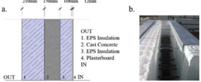
ICF is classed among the site-based Modern Methods of Construction (MMC) [29]. Although it dates back in Europe since the late 1960's, it is often characterised as an innovative wall technology because it has only recently become more popular for use in residential and commercial construction [30]. The ICF wall component consists of modular pre-fabricated Expanded Polystyrene Insulation (EPS) hollow blocks and cast in situ concrete (Fig. 1). The blocks are assembled on site and the concrete is poured into the void. Once the concrete has cured, the in-sulating formwork stays in place permanently. The resulting construc-tion structurally resembles a convenconstruc-tional reinforced concrete wall.
The ICF wall system has several advantages; apart from its increased speed of construction and its strength and durability, ICF can provide complete external and internal wall insulation, minimising the ex-istence of thermal bridging, providing very low U-values and high
levels of air-tightness if installed correctly [29,31]. ICF is generally perceived as merely an insulated panel, acting thermally as a light-weight structure. There is the general perception that the internal layer of insulation isolates the thermal mass of the concrete from the internal space and interferes with their thermal interaction. Nonetheless, pre-vious computational, numerical and field studies, indicate that the thermal capacity of its concrete core shows evidence of heat storage effects, which in specific climatic and building cases, could result ulti-mately in reduced energy consumption when compared to a lightweight conventional timber-framed wall with equal levels of insulation [25,30,32–38].
Fig. 1contrasts a typical cross section, as used in the representation of ICF in numerical simulations against the reality of prefabricated blocks of EPS. The insulation layers are connected with plastic ties, creating the void, where the concrete will then be poured. Thefigure illustrates one example of possible simplifications when a construction is represented in a model and how it differs from reality and increases the level of modelling uncertainties.
1.3. Building modelling, simulation and uncertainty
It is common to see the words“simulation”and“modelling”used interchangeably. However, they are not synonyms. Becker and Parker [39] defined simulation as the process that implements and instantiates a model. Instead, modelling is the representation of a system that contains objects that interact with each other. A model is often math-ematical and describes the system that is to be simulated at a certain level of abstraction. Within a BPS program descriptions of the con-struction, occupancy patterns and HVAC systems are given and a mathematical model is constructed to represent the possible energy flow-path and their interactions [7,11]. Many assumptions, approx-imations and compromises are inevitably made on the mathematical formulations describing the physical laws within the model [40]. Consequently an exact replication of reality should not be expected. There is often a discrepancy between expected energy performance during design stage and real energy performance after project com-pletion [41]. Moreover, there are often inconsistencies in the simulation results when modelling an identical building using different BPS tools, referred to as modelling uncertainties [42]. These can lead to a lack of confidence in building simulation.
Previous research on the uncertainty of simulation predictions concluded that the reliability of simulation outcomes depends on the accuracy and precision of input data, simulation models and the skills of the energy modeller [43–46]. An estimation of the uncertainty in-troduced by each of the aforementioned factors can help to increase the awareness of the results reliability. Quality assurance procedures and consideration of the inherent uncertainties in the inputs and modelling assumptions are two areas that require attention in BPS.
There are a vast number of previous studies analysing the various sources of uncertainty in BPS results. De Wit classified the sources of uncertainty as follows [47]:
•
Specification uncertainties, associated to incomplete or inaccurate specification of building input parameters (i.e. geometry, material properties etc.)•
Modelling uncertainties, defined as the simplifications and assump-tions of complex physical processes (i.e. zoning, scheduling, algo-rithms etc.)•
Numerical uncertainties, all the errors that are introduced in the discretisation and the simulation model.•
Scenario uncertainties, which are in essence all the external condi-tions imposed on the building (i.e. weather condicondi-tions, occupants behaviour).uncertainty analysis into ESP-r [48]. Hopfe and Hensen investigated the possibility of supporting design by applying uncertainty analysis in building performance simulation [42]. Prada et al., studied the effect of uncertain thermophysical properties on the numerical solutions of the heat equation, analysing the difference between Conduction Transfer Functions (CTF) and Finite Difference (FD) model predictions [46]. Mirsadeghi et al., reviewed the uncertainty introduced by the different external convective heat transfer coefficient models in building energy simulation programs [49]. Silva and Ghisi, examined the discrepancies in the simulation results due to simplifications in the geometry of a computer model [50]. Gaetani et al. [51,52], investigated the un-certainty and sensitivity of building performance predictions to dif-ferent aspects of occupant behaviour, by separating influential and non-influential factors. Kokogiannakis et al. [53], compared the simplified methods used for compliance as described in ISO 13790 standard with two detailed modelling programs (i.e. ESP-r and EnergyPlus). The aim was to determine the magnitude of differences due to the choice of simulation program and whether the different methods under in-vestigation would lead to different compliance conclusions. Irving in-vestigated several aspects that are related to the validation of dynamic thermal models [40]. Among others, the author highlighted the infl u-ence of users in the accuracy of BPS results. The author suggested that even if a model is completely accurate, errors may still arise because little guidance is usually available on how to use the model properly. Guyon et al., also studied the role of model user in BPS results, by comparing the results provided by 12 users for the same validation exercise [54]. They concluded that the user's experience affected the results variations. A good homogeneity was found among the different categories of participants' expertise. The impact of modeller's decision on the simulation results was also studied by Berkeley et al., [55]. The authors found that the results provided by 12 professional energy modellers for both the total yearly electrical and gas consumption varied significantly.
1.4. Aim of paper
There is a wide range of scientifically validated1BPS tools available
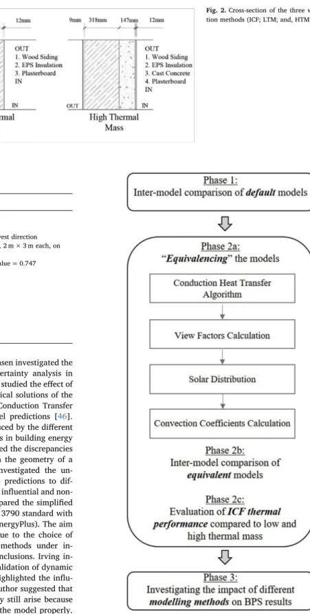
Fig. 2.Cross-section of the three wall construc-tion methods (ICF; LTM; and, HTM).
Table 1
Input data used for the building model. Building Model Details
Internal Treated Floor Area
6 m × 8 m = 48m2
Orientation Principal axis running east west direction Windows Two double glazed windows, 2 m × 3 m each, on
south façade,
U-Value = 3.00 W/m2K, g-Value = 0.747
U-Values (W/m2K) Walls = 0.10
Floor = 0.10 Ceiling = 0.11 HVAC system Ideal loads
HVAC Set points 20 °C Heating/27 °C Cooling HVAC Schedule 24 h (Continuously on) Internal Gains 200 W (other equipment) Infiltration 0.5ACH (Constant)
Fig. 3.The three phases in the research method.
1Tools that have been shown to pass certain validation tests (i.e. analytical tests,
on the market. Some of the tools are simple and more“user-friendly”, others are more detailed, requiring an advanced level of expertise and experience from the modeller. In several cases, there are assumptions embedded in the BPS programme that are outside the modeller's con-trol. In other cases, the modeller is required to make a decision on whether to rely on the default settings of a tool or to specify the solution algorithms and values that are to be used in the simulations. The ana-lysis presented in this paper investigates the implications of the
“modelling gap”, the different modelling methods on the simulation of three different types of thermal mass in whole BPS using two different tools. Focussingfirstly on the impact of default input parameters and then on the effects of the various calculation algorithms on the results divergence, the purpose is to examine the disparity of different mod-elling assumptions. The order of magnitude of the problem faced by the modeller during the specification of a building is shown, focussing on the representation of thermal mass in building simulation. The focus is particularly on the simulation of ICF; a construction method which is not yet well-researched. To the authors' knowledge this is the first thorough investigation of the simulation of ICF and thefirst study that reflects on the effect of modelling decisions and modelling uncertainty on thermal mass simulation.
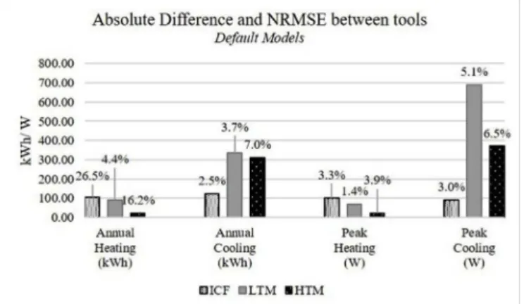
2. Research method
The case study was a single-zone test building based on the one specified in the BESTEST methodology [56]. The rationale was to minimise building complexity and thus decrease the number of vari-ables related to geometry and zoning in the input data. At the outset, all simulation models were validated using the BESTEST case 600 for low thermal mass and case 900 for high thermal mass. Then the construc-tion details were changed in line with the specific study. All other input parameters remained identical to the BESTEST methodology. Three different construction methods: insulated concrete formwork, low thermal mass, and high thermal mass were simulated, as shown in
Fig. 2. For ease of reference, these will be referred to as ICF, LTM and HTM from this point forward.
The ICF option was based on real building construction details, and was used as a reference to specify U-Values for all other construction elements. In this way U-values were consistent for all three building models; hence, the main difference between the three construction methods was in the amount of thermal mass. Table A.1(in the Ap-pendix) describes the construction materials for all three options.
The simulation settings were identical in all three scenarios: each building model had the same internal footprint, window size and glazing properties, the same HVAC system, internal gains and infi ltra-tion rates, as summarised inTable 1. Energy was used for space con-ditioning and other equipment. No domestic hot water was used. The DRYCOLD weatherfile, downloaded from NREL,2was used as a Typical Meteorological Year (TMY), i.e. a climate with cold clear winters and hot dry summers.
Two freeware, validated and commonly used BPS tools were se-lected, as they showed the greatest overall consistency in setup and default settings (seven other tools were considered and discounted) [33]. Importantly, both tools offered significantflexibility to the user, through changing the default settings, hence they presented the best opportunity to achieve the overall aim of the research. These will be referred to as tools A and B from this point onwards.
The research was undertaken in three main phases, as shown in
Fig. 3.
Phase 1 compared simulation results provided by the two BPS tools when simulating all three construction methods (i.e. ICF, LTM, and HTM) using the tools' default algorithms. This was done to determine whether any discrepancies in the simulation predictions provided by
the tools were significant (i.e. surface temperatures, heating or cooling demand), and whether this discrepancy was affected by the amount of thermal mass. Both annual and hourly results were included in the analysis:
1. Results for the annual energy consumption and the peak thermal loads were plotted monthly. Divergence in the simulation predic-tions was analysed using the Normalised Root Mean Square Error (NRMSE) (1). The NRMSE3is a non-dimensional form of the RMSE and was used to calculate absolute error in simulation results.
= ∗ ∑= − NRMSE x (%) 100 x x n ( ) i n i b i a 1 , , 2 (1) = + x x x 2 i i a, i b, (2) = ∑= x x n i n i 1 (3) Where,
xi a, andxi b, are the predictions provided by tools A and B respec-tively at each time step
xiis the mean value ofxi a, andxi b, for each time step
x is the mean value of the predictions provided by both tools A and B
nis the size of the sample
2. Hourly results for the heating and cooling demand, along with surface temperatures of a wall element were plotted for two three-day periods, one in the heating and one in the cooling season. The days selected for the hourly results analysis were when the highest and lowest dry-bulb outdoor temperatures were recorded. The analysis focussed on the internal surface, intra-fabric and external surface temperature of the east wall. The east wall was selected for this step of the analysis because it would receive direct solar ra-diation both in its external and internal surfaces. However, a rela-tively similar divergence was observed in the results provided by the two BPS tools for all other walls in the simulation models. Phase 2 focussed on the model“equivalencing”process. This was done to minimise any differences between the simulation models, making them equivalent for comparison, by selecting identical algo-rithms and consistent input settings (seeTable A.2in the Appendix). An extended literature review identified the main features, capabilities and default solution algorithms in the tools [6,57]. An overview of the calculation and solution algorithms employed in both BPS tools is in-cluded inTable A.3(Appendix). The“equivalencing”process was done on the annual simulation results, aiming to serve as a crude analysis on the impact of the different algorithms on the results discrepancy. Starting from a basecase scenario representing the default models, a step-by-step process was followed to make the models equivalent by changing to identical solution algorithms one step at a time. The impact of each step was investigated by calculating the NRMSE, for each of the three construction methods. The results were analysed sequentially to understand which algorithms had the greatest impact on each dis-crepancy, how the inconsistencies were affected based on the varying levels of thermal mass, and whether any divergence became more ob-vious (i.e. heating or cooling demand). Once the simulation models were“equivalenced”, the NRMSE of the annual and hourly results were compared against the initial NRMSE of the default models. The aim was to quantify the reduction in the results variation.
The thermal performance of the ICF, LTM and HTM models were
compared before and after the model “equivalencing” process. The purpose was to investigate if the results would be different pre and
post-“equivalencing”, to reflect on the impact of the“modelling gap”and to highlight the significance of reducing uncertainties in building perfor-mance simulation.
Following the model “equivalencing” process, several modelling factors that were found to have a significant impact on the results were investigated further. Therefore, the third andfinal phase considered the differences in modelling methods employed by the two tools. This was done to highlight how the simulation outcome is affected by the dif-ferent modelling methods, even when the input values are identical (in this instance the climate data).
3. Results and analysis
This section presents the results obtained from the three phases of the research. Annual and hourly simulation results obtained by the two BPS tools when the user relies on the default setting are presentedfirst. Then, the simulation predictions of the equivalent models are analysed, followed by an account of the investigation of the different modelling methods available within the two BPS tools. The purpose of the section is to provide a detailed account of the outcomes of the analysis, in particular to consider the differences between tools A and B.
3.1. Phase 1: impact of default settings on the BPS results
3.1.1. Annual simulation results of two tools using default settings
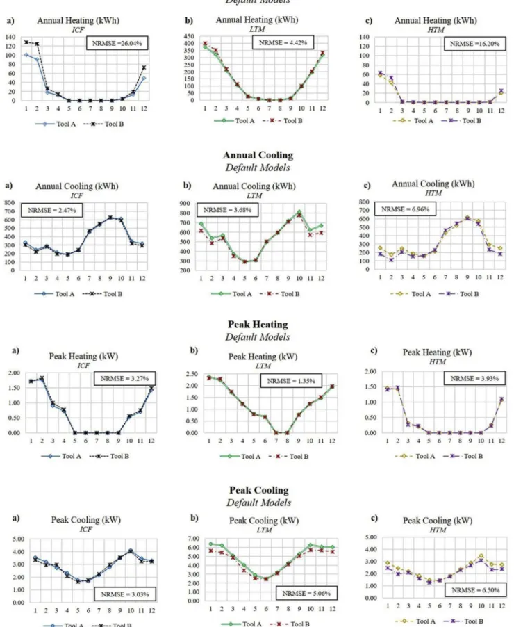
The following section analysed the annual simulation results for the heating and cooling demand provided by the two tools, when the user relies on the default settings and their variation.Fig. 4shows the ab-solute difference and the NRMSE in the simulation results provided by tools A and B for each construction method, for the annual heating and cooling energy consumption and the peak heating and cooling loads. The divergence in the simulation results provided by the two tools for the default models was high. In terms of absolute difference in the annual and peak heating demand, the ICF building showed the highest difference in the simulation predictions provided by the two tools. In the annual and peak cooling demand, the highest absolute difference (in kWh and W) was observed in the LTM building, followed by the HTM building. In general the absolute differences were higher in the annual and peak cooling demand, reaching up to 300 kWh in the annual cooling demand of the LTM and HTM buildings and up to 700 W in the peak cooling demand of the LTM building.
Looking at the relative differences (i.e. NRMSE) in the predictions
provided by the two BPS tools, highlighted the significance of these variations. The largest divergence was found in the annual heating energy consumption for ICF (NRMSE = 26.05%) and HTM (NRMSE = 16.20%). Furthermore, the HTM case showed a major dif-ference in the annual cooling and peak cooling loads (NRMSE = 6.96% and NRMSE = 6.50% respectively). The LTM building showed overall good consistency in the simulation predictions for both annual energy consumption and peak loads, with the exception of peak cooling de-mand (NRMSE = 5.06%). Finally, there was good agreement between the two tools for the peak heating loads, regardless of the amount of thermal mass (NRMSE < 4%).
The monthly breakdown of annual heating energy consumption for the default models, as illustrated inFig. 5, shows that the greatest di-vergence was found in results for the winter months (December, Jan-uary and FebrJan-uary); it was most significant in the ICF and the HTM buildings. In the monthly breakdown of the annual cooling energy consumption (Fig. 5) the predictions for ICF showed good consistency. The most significant discrepancy was observed in LTM and HTM be-tween January and April, and bebe-tween November and December. Good agreement between the two BPS tools was achieved over the summer period. For peak heating loads (Fig. 5), the divergence was negligible during the entire simulation period, for all three constructions. For peak cooling loads (Fig. 5), the ICF case showed an insignificant variation between the two tools, whereas the other two construction methods (i.e. LTM and HTM), displayed a surprisingly high divergence in peak cooling loads during the heating period (January to May and October to December), yet there is a good consistency over the summer months.
3.1.2. Hourly simulation results of the two BPS tools relying on the default settings
Fig. 6shows the discrepancy in the hourly simulation results pro-vided by the two BPS tools for the internal surface, the intra-fabric4and the external surface temperatures of the east wall. The results are plotted for three consecutive days in the heating period, when the lowest outside dry-bulb temperature was predicted. The divergence in the predictions of the two tools was relatively low for the internal surface temperature in all three constructions, with a maximum of NRMSE5= 4.00% observed in the ICF building. The node temperature in the middle of the wall element showed that there was a more pro-nounced discrepancy in the LTM building (NRMSE = 29%), much lower compared to the other two construction methods, where the variation was NRMSE = 4.71% for the ICF and just NRMSE = 1.82% for the HTM building. With regards to the outside surface temperature, the same variation equal to NRMSE = 12% was observed in all three constructions.
Fig. 7shows the discrepancy in the simulation predictions provided by the two BPS tools for the inside surface, intra-fabric and outside surface of the east wall for three consecutive days in the cooling season. The variation in the temperature of the internal surface was negligible in all three constructions (below NRMSE = 2%). There was an NRMSE = 5% discrepancy in the predictions of the intra-fabric tem-perature of the LTM wall. Finally, there was an NMRSE = 8.75% dis-crepancy in the simulation of the outside surface temperature, which was again found to be the same in all three construction methods.
It is noteworthy that although the divergence in the simulation predictions provided by the two BPS tools was relatively low with re-gards to hourly temperature results, looking at the absolute divergence, there were instances that the maximum temperature difference was high. For example looking at the internal surface of the ICF building, as
Fig. 4.Absolute Difference and NRMSE between the simulation predictions provided by tools A and B for the three construction methods, when the user relies on the tools' default settings.
4Tool A calculates by default the conduction heat transfer using the Conduction
Transfer Function algorithm. CTF does not allow the calculation of temperature dis-tribution within the element of the fabric. For the purposes of this analysis, the con-duction heat transfer algorithm for the East wall was set to Concon-duction Finite Difference.
5The hourly temperature results are expressed in degree centigrade throughout the
Fig. 5.Monthly breakdown of annual heating and cooling energy consumption and peak heating and cooling loads. Simulation predictions provided by tool A and tool B for all three constructions: (a) ICF, (b) low thermal mass (LTM) and (c) high thermal mass (HTM), when the user relies on the tools' default settings.
predicted by the two tools (Fig. 6), the maximum absolute difference reached up to 5 °C. Thisfinding could affect significantly the outcome of thermal comfort assessments and the selection of BPS tools could result in different conclusions regarding the thermal performance of the building.
The discrepancy in the predictions of the east wall temperature evolution was relatively low in all three construction methods (apart from the intra-fabric temperature of the LTM wall in the heating season). In general, the discrepancy in the results for the wall tem-perature was found to be higher in the LTM building than the other two
Fig. 6.Hourly breakdown of the inside surface, intra-fabric and outside surface temperature of the east wall. Simulation predictions provided by tool A and B for three consecutive days in the heating season (03–05 January) for all three constructions: (a) ICF, (b) low thermal mass (LTM) and (c) high thermal mass (HTM), when the user relies on the tools' default settings.
construction methods. As a result it would be expected that the varia-tion in the heating demand predicvaria-tions would also be higher in the LTM building. Surprisingly, the hourly breakdown of the heating demand, as indicated inFig. 8, showed that there was an NRMSE = 13.43% for the
ICF building, an NRMSE = 9.20% for the HTM building and the LTM building showed the lowest variation equal to NRMSE = 5.16%.
The discrepancy in the simulation predictions for the hourly cooling demand in the three-day cooling period as shown in Fig. 9 was
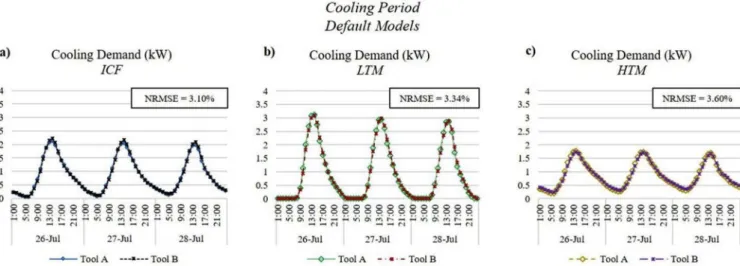
Fig. 7.Hourly breakdown of the inside surface, intra-fabric and outside surface temperature of the east wall. Simulation predictions provided by tool A and B for three consecutive days in the cooling season (26–28 July) for all three constructions: (a) ICF, (b) low thermal mass (LTM) and (c) high thermal mass (HTM), when the user relies on the tools' default settings.
relatively low for all three construction methods, even when the user relies on the default setting of the tools.
3.2. Phase 2: simulation results of equivalent models
3.2.1. “Equivalencing”the models
Prior to analysing the various calculation algorithms and their im-pact on the results divergence, it was essential to minimise the diff er-ences in the two models, caused by other factors. As part of the
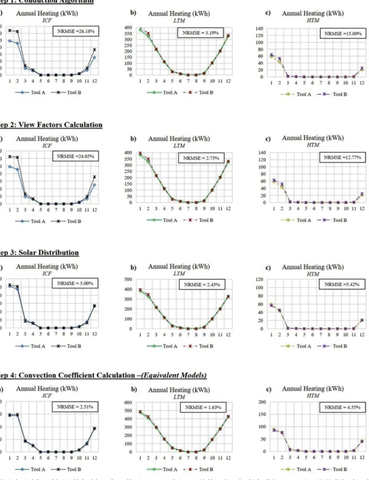
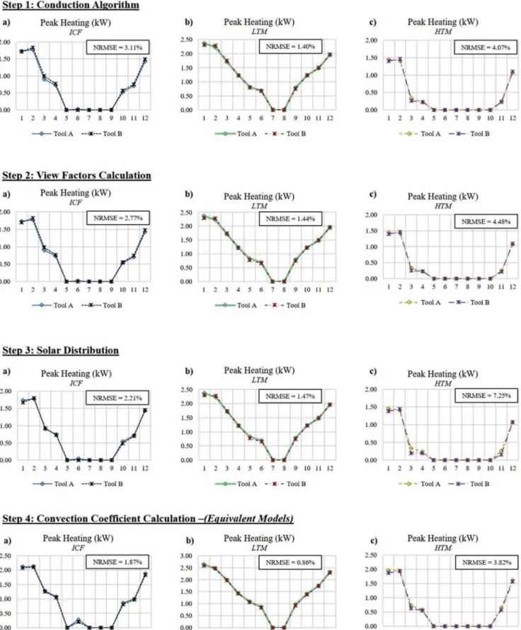
“equivalencing”process, Figs. 10–13 show the various steps used to minimise the difference between the two tools, i.e. to make the models equivalent for comparison. Results are shown for all three construction methods (ICF, LTM, and HTM), for each tool, along with the NRMSE.
Fig. 10 shows the process of making the models equivalent and its impact on the monthly breakdown of annual heating energy con-sumption. Fig. 11shows the“equivalencing” progression for annual cooling energy consumption.Figs. 12 and 13show“equivalencing”in the peak heating and peak cooling demands, respectively.
In every case the “equivalencing” process resulted in reasonably consistent simulation results provided by the two BPS tools for the
equivalent models (Step 4inFigs. 10–13). The largest discrepancy was observed in the annual heating and cooling demand of the HTM building. A step-by-step process was followed to make the models equivalent by changing to identical solution algorithms.
•
InStep 1the conduction heat transfer algorithm in tool A was set to finite difference to match the conduction heat transfer calculation of tool B. This reduced the variation in the predictions for annual heating energy consumption in the LTM and HTM buildings, yet it increased the NRMSE in the ICF case (compared to the default models inFig. 9). The NRMSE was also increased in the predictions for the annual cooling demand for ICF and LTM, while it was re-duced in the HTM building. Moreover, the discrepancy increased in predictions for the peak cooling loads for all three constructions.•
InStep 2the same view factors, used to calculate the radiant heatexchange between surfaces, were set in both models. This reduced the NRMSE in all cases, for all three constructions, apart from the peak heating loads, where it was slightly increased for LTM and HTM.
•
InStep 3the direct solar distribution falling on each surface in theFig. 8.Hourly breakdown of heating demand. Simulation predictions provided by tool A and B for three consecutive days in the heating season (03–05 January) for all three con-structions: (a) ICF, (b) low thermal mass (LTM) and (c) high thermal mass (HTM), when the user relies on the tools' default settings.
Fig. 9.Hourly breakdown of cooling demand. Simulation predictions provided by tool A and B for three consecutive days in the cooling season (26–28 July) for all three constructions: (a) ICF, (b) low thermal mass (LTM) and (c) high thermal mass (HTM), when the user relies on the tools' default settings.
Fig. 10.“Equivalencing”the models. Monthly breakdown of annual heating energy predictions provided by tool A and tool B for all three constructions: (a) ICF, (b) low thermal mass (LTM) and (c) high thermal mass (HTM).
Fig. 11.“Equivalencing”the models. Monthly break down of annual cooling energy predictions provided by tool A and tool B for all three constructions: (a) ICF, (b) low thermal mass (LTM) and (c) high thermal mass (HTM).
Fig. 12.“Equivalencing”the models. Monthly break down of peak heating loads predictions provided by tool A and tool B for all three constructions: (a) ICF, (b) low thermal mass (LTM) and (c) high thermal mass (HTM).
Fig. 13.“Equivalencing”the models. Monthly break down of peak cooling loads predictions provided by tool A and tool B for all three constructions: (a) ICF, (b) low thermal mass (LTM) and (c) high thermal mass (HTM).
zone, including floor, walls and windows was calculated in both models by projecting the sun's rays through the exterior windows. This step significantly affected all the results. The NRMSE in the predictions was notably reduced in almost every case, particularly in the annual heating energy consumption. However, the NRMSE in the peak heating was increased in the HTM case.
•
Finally, in Step 4 the convection coefficients of the internal and external surfaces, used to calculate the convection heat transfer, were set to the same constant user-defined values. This, surprisingly, increased the variation for the annual cooling energy consumption and decreased the discrepancy in the annual heating and the peak loads for all three constructions. Furthermore, a general observation is that, by setting the surface convection coefficients to constant, the energy consumption predicted by both tools for the annual and the peak heating demand for all three construction methods increased considerably, whereas the annual and peak cooling demand re-mained unaffected. Assuming constant values for the convection coefficients was a limitation of this study. In reality the building is always exposed to changes in the boundary conditions, resulting in time-varying convective transfer coefficients [58]. However, for the purpose of this analysis, where the aim was to minimise the diff er-ences between the two BPS tools as much as possible, constant convection coefficients were used in order to reduce the level of modelling uncertainty.3.2.2. Annual simulation results of equivalent models
Following the model“equivalencing” process, the profiles of the monthly breakdown for the annual heating demand of the equivalent models (Step 4inFig. 10) show that the most pronounced discrepancy was found again in the winter months (January to February), especially in the ICF building. In the annual cooling energy consumption however (Step 4ofFig. 11), the greatest divergence in the equivalent models was observed between July and October in all three construction methods, and was more obvious in the ICF and HTM cases. Contrary to the de-fault models, an overall good agreement was observed in the annual cooling results of the two BPS tools during the winter period. In the peak heating and peak cooling loads (Step 4inFigs. 12and13) the
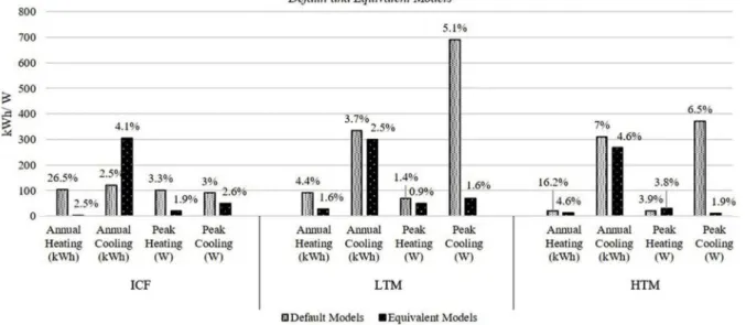
NRMSE was insignificant and no substantial discrepancy was evident. The divergence in the annual simulation results for the equivalent models was reduced compared to the default models (Fig. 14) in both heating and cooling demand and for all construction methods.Fig. 14
shows the absolute difference and the NRMSE in the simulation pre-dictions provided by tools A and B for annual heating and cooling en-ergy consumption and peak heating and cooling loads for both the default and the equivalent models. The graph illustrates how the ab-solute difference and the NRMSE were reduced in the equivalent models for all three construction types, in instances up to 24% (i.e. annual heating of ICF). With regards to the absolute differences, the highest discrepancy in the prediction of the two tools was observed in the annual cooling demand, reaching up to 300 kWh for all three con-struction methods. This value might be considered as high, yet when compared to the total calculated annual cooling demand (i.e. varies between 4000 kWh for the HTM and to 7000 kWh for the LTM build-ings) it is of less significance. In the annual heating, peak heating and peak cooling demand the absolute differences were minimised for all three buildings. Looking at the relative differences in the predictions provided by the two BPS tools, the highest divergence was observed in the annual heating and cooling energy consumption of HTM and the annual cooling demand of the ICF building (NRMSE = 4.6% and NRMSE = 4.1%, respectively). In general, the simulation results pro-vided by the equivalent models for all three construction methods were very consistent. However, the discrepancy in the prediction of the an-nual cooling demand remained high in all three constructions even after the models were“equivalenced”. Particularly in the case of ICF, the divergence in the calculation of the annual cooling demand increased after the“equivalencing”process rather than decreasing.
3.2.3. Hourly simulation results of equivalent models
Fig. 15andFig. 16show the discrepancy in the hourly simulation results provided by the two BPS tools for the internal surface, the intra-fabric and the external surface temperatures of the east wall after the
“equivalencing”process.Fig. 15shows the results for three consecutive days in the heating period. As can be seen from the graphs the variation in the predictions for all three constructions was very low for the
Fig. 14.Absolute difference and NRMSE between the simulation predictions provided by tools A and B for the three construction methods, (i) ICF, (ii) low thermal mass (LTM) and (iii) high thermal mass(HTM), when the user relies on the tools' default settings and when the models are equivalent.
temperatures of the three nodes (i.e. inside surface, intra-fabric and outside surface). A very good consistency was achieved in the results provided by the two BPS tools. The highest variation was found in the outside surface temperature, where the NRMSE = 3.00%, yet it was still relatively low.
An even better agreement between the two tools was achieved for the prediction of the surface temperatures in the cooling period (Fig. 16). The variation in the temperature of the nodes for all three case, inside surface, intra-fabric and outside surface was found to be negligible in all three constructions (below NRMSE = 2%).
Fig. 15.Hourly breakdown of the inside surface, intra-fabric and outside surface temperature of the east wall. Simulation predictions provided by tool A and B for three consecutive days in the heating season (03–05 January) for all three constructions: (a) ICF, (b) low thermal mass (LTM) and (c) high thermal mass (HTM), when the models are equivalent.
The absolute differences in the internal, intra-fabric and external temperatures, as predicted by the two BPS tools, were also negligible for both periods under investigation and for all three construction methods.
With regards to the hourly breakdown of the heating and cooling demand, as illustrated inFig. 17andFig. 18, there was again a very good agreement in the predictions provided by the two BPS tools. For the heating demand (Fig. 17) the discrepancy was found to be lower
Fig. 16.Hourly breakdown of the inside surface, intra-fabric and outside surface temperature of the east wall. Simulation predictions provided by tool A and B for three consecutive days in the cooling season (26–28 July) for all three constructions: (a) ICF, (b) low thermal mass (LTM) and (c) high thermal mass (HTM), when the models are equivalent.
than NRMSE = 4.50% for all three construction methods. The variation in the cooling demand (Fig. 18) was found to be even lower and around NRMSE = 2.50% for all three buildings. The general observation is the after the model were equivalenced, there was a very good consistency in the hourly simulation predictions both for the surface temperatures, but also for the space heating and cooling needs.
3.2.4. Comparison of thermal performance between the three constructions
A comparison was performed on the annual thermal performance of ICF against the thermal performance of the LTM and the HTM building, before and after the model “equivalencing”process. The aim was to investigate whether the“modelling gap”would affect the conclusions on the comparative performance of ICF and to highlight the significance of reducing uncertainties in building performance simulation. The re-sults illustrated inFigs. 19 and 20show the average in the simulation predictions provided by the two BPS tools for the default and equivalent models, respectively.Tables 2 and 3summarise the percentage diff er-ence in energy consumption of ICF compared to LTM and HTM, as
Fig. 17.Hourly breakdown of heating demand. Simulation predictions provided by tool A and B for three consecutive days in the heating season (03–05 January) for all three constructions: (a) ICF, (b) low thermal mass (LTM) and (c) high thermal mass (HTM), when the models are equivalent.
Fig. 18.Hourly breakdown of cooling demand. Simulation predictions provided by tool A and B for three consecutive days in the cooling season (26–28 July) for all three constructions: (a) ICF, (b) low thermal mass (LTM) and (c) high thermal mass (HTM), when the models are equivalent.
Fig. 19.Comparison of ICF building energy consumption to LTM and HTM buildings, when the user relies on the tools' default settings, average of both tools.
predicted by each two BPS tools (along with their average).
Fig. 19andTable 2show the comparison between ICF, LTM and HTM buildings when the user relies on the default settings of the tools. Comparing the overall annual heating demand of ICF to the other two construction methods, the two BPS tools predicted that ICF would re-quire on average 80.5% less annual heating energy than LTM and 60% more than HTM. In the annual cooling energy consumption, ICF showed 33.5% less cooling demand than the LTM building and 13.5% more than the HTM building. The peak heating loads of the ICF building were 25.5% less compared to the LTM building and 18% higher than the HTM. Finally, in the peak cooling loads ICF showed 33.5% reduced
After the models“equivalencing”process the results, as shown in
Fig. 20 and Table 3, indicate that ICF behaves closer to the HTM building than before. For instance, in the annual heating demand, the two BPS tools predicted that ICF would require on average 56% more energy than the HTM building. Thisfigure remains high, yet it is lower than the initial estimations pre-equivalencing (Table 2). Accordingly, post-equivalencing the ICF building showed 8% increased peak heating demand compared to the HTM building (Table 3). Pre-equivalencing this value was estimated to be 18% (Table 2). Similarfindings apply to the peak cooling demand. The general remark both before and after the model“equivalencing”process is that the ICF building behaved much more similarly to HTM, with the exception of annual heating energy consumption. For annual heating demand, although the energy con-sumption of ICF was significantly reduced compared to LTM (78.5%), it still required higher amount of heating energy compared to HTM (56%). In the annual cooling demand and the peak heating and cooling loads ICF consumed slightly increased energy than the heavyweight structure. In the comparison of ICF to LTM, the former consumed sig-nificantly less energy for both annual heating and cooling.
Looking at the monthly breakdown of the annual and peak, heating and cooling demand for the equivalent models (Step 4ofFigs. 10–13), the thermal performance and the energy consumption of ICF was compared to the other two options. For annual heating energy con-sumption (Step 4inFig. 10), the profiles of the monthly breakdown is similar for all three constructions, although the amount of heating de-mand varies significantly. More specifically, LTM requires a maximum of around 500 kWh of heating during January, while ICF and HTM require approximately 150 kWh and 80 kWh respectively. Moreover, the LTM results indicated no heating demand for two months, July and August, and for ICF there was no heating demand forfive months (i.e. May to September). For HTM, the heating demand was even smaller and the results predicted zero heating for seven months, between May and November.
In the annual cooling energy consumption (Step 4ofFig. 11), ICF and HTM followed very similar profiles in the monthly breakdown and require similar amounts of cooling. LTM indicated a different profile of annual cooling compared to the other two cases, throughout the year. In general, it required more cooling energy, with higher peaks, espe-cially over the heating period (i.e. January to May, September to De-cember).
In respect of peak heating loads (Step 4ofFig. 12), all three con-struction methods showed different monthly profiles. As with the an-nual heating demand, in the peak heating loads, LTM indicated no heating demand for two months, in July and August. The ICF building required no heating for almostfive months (May to September), while HTM indicated no peak heating loads over a period of six months (May to October). LTM required a maximum peak heating of around 2.50 kW in January, while for the other two methods the maximum demand (of around 2.00 kW) occurred in February. In general LTM showed in-creased peak heating demand throughout the year compared to the other two buildings. ICF and HTM required relatively similar amounts of heating over winter and summer, with the main differences found to be over the intermediate periods (March to May and September to November).
For peak cooling loads (Step 4of Fig. 13), all three constructions showed a similar profile in the monthly breakdown, with the exception of November and December, when there was a significant drop in the peak cooling loads for ICF and HTM, yet for LTM the demand remained almost constant. The amount of peak cooling in LTM was higher com-pared to the other two cases, throughout the year.
Looking at the difference in predicted performance of ICF compared to the other two construction methods due to the use of different tools, before and after the model “equivalencing” process, as indicated in
Tables 2 and 3, it is obvious that a very good consistency was achieved
Fig. 20.Comparison of ICF building energy consumption to LTM and HTM buildings, when the models are equivalent, average of both tools.
Table 2
Percentage difference in energy consumption of ICF compared to LTM and HTM, when the user relies on the tools' default settings.
ICF Energy Consumption
ICF vs. LTM ICF vs. HTM Tool A Tool B Average of
both Tools
Tool A Tool B Average of both Tools Annual Heating −83% −78% −80.5% +57% +63% +60% Annual Cooling −33% −34% −33.5% +11% +16% +13.5% Peak Heating Loads −27% −24% −25.5% +16% +20% +18% Peak Cooling Loads −36% −31% −33.5% +15% +23% +19% Table 3
Percentage difference in energy consumption of ICF compared to LTM and HTM, when the models are equivalent.
ICF Energy Consumption
ICF vs. LTM ICF vs. HTM Tool A Tool B Average of
both Tools
Tool A Tool B Average of both Tools Annual Heating −78% −79% −78.5% +55% +57% +56% Annual Cooling −37% −37% −37% +14% +14% +14% Peak Heating Loads −19% −19% −19% +8% +8% +8% Peak Cooling Loads −34% −33% −33.5% +13% +15% +14%
variation between the two tools was around 6% in the annual heating, 4% in the annual cooling and peak heating loads and up to 8% in the peak cooling loads. After the models were“equivalenced”the variations in the predicted performance provided by the two BPS tools were minimised to less than 2%. Similarfindings apply to the comparative performance of ICF to LTM construction method. In general, the
“equivalencing” process resulted in more consistent conclusions re-garding the energy consumption of ICF compared to the other two construction methods.
3.3. Phase 3: investigating the impact of different modelling methods on BPS results
During the“equivalencing”process, several observations were made in respect of the different modelling methods employed by the two BPS tools–this section provides an overview of some important points.
Thefirst was the solar timing that was used in the calculation of the solar data. In both tools the solar values in the weather file were average values over the hour. When the simulation timestep was greater than 1 (sub-hourly simulation), interpolated values were used. Tool A calculated by default the average values based on the midpoint of each hour, whereas tool B offered a user-selectable option to treat solar irradiance included in the climatefiles, based on the half hour or the top of each hour. As a consequence, the selection of the solar timing calculation affected the simulation results provided by tool B.Fig. 21, shows the comparison of the simulation predictions provided by tool B when the solar timing was set to the midpoint or the top of the hour, for annual and peak heating demand (Fig. 21a) and annual and peak cooling demand (Fig. 21b). The hatched bars show the results when
solar timing is taken at the midpoint of the hour and the solid-coloured bars show the results when solar timing is taken at the top of each hour. For all three construction methods, the annual and the peak heating demand was always reduced when the solar timing was set to the midpoint of the hour, but the annual and peak cooling was slightly increased.Fig. 21a shows some very clear differences in the predicted annual heating demand due to solar timing calculations for all three construction methods. The maximum difference, as indicated in
Table 4, was in the annual heating energy consumption of the HTM and the ICF buildings (−7.48% and−6.23% respectively). In general there were insignificant differences in the annual and peak cooling demand; hence the solar timing had only a minor impact on the cooling pre-dictions.
Another factor that was investigated as part of the“equivalencing”
process was the impact of assumptions for the calculation of the ex-ternal surface convection coefficients; more specifically, the impact of variations in wind speed on the simulation results provided by the two
Fig. 21.Absolute difference in the predictions provided by tool B when solar timing is set to the midpoint or the top of the hour. (a) Annual and peak heating demand, (b) Annual and peak cooling demand.
Table 4
Relative difference in the predictions provided by tool B when solar timing is set to the midpoint or the top of the hour.
Solar Timing Calculation Relative Difference
Annual Heating Peak Heating Annual Cooling Peak Cooling ICF −6.23% −0.32% +0.30% +0.05% LTM −3.27% −0.41% +0.14% +0.13% HTM −7.48% −0.62% +1.18% +1.10%
BPS tools. When the external convection coefficient of the surfaces was set to constant (user-defined), the variations in the wind speed (i.e. taken from the climatefile), had no impact on the simulation results, as anticipated. In other words, assuming a constant exterior convective coefficient, could be interpreted as setting a constant value for the wind velocity throughout the simulation period. However, when the con-vection coefficients were calculated based on the default algorithms, the impact of wind speed differed between the two tools and varied according to the construction method. The reason was that both tools consider the wind speed in their external surface convection coefficient calculation regime, yet they use different equations to do so. Tool A included surface roughness within the external convection coefficient calculation, whereas tool B relied solely on the wind speed. To in-vestigate this issue further, the default algorithms for the calculation of convective heat transfer coefficients were selected in both tools and the simulations were performed twice; once when the wind speed was taken from the climatefile and once when the wind speed in the climate file was set to 0 m/s throughout the whole year.
Fig. 22 shows the impact of the assumptions for convective heat transfer coefficients on the results provided by tool A and tool B, for annual and peak heating demand and annual and peak cooling demand. The graphs illustrate the absolute difference in kWh (annual demand) and in W (peak loads) when the wind speed is taken from the climate file and when the wind speed is set to 0 m/s throughout the simulation period. The solid-coloured bars show the reduction (or increase) in the results due to the lack of wind for tool A and the hatched bars show the reduction (or increase) for tool B. Here, annual and peak heating de-mand was reduced in the absence of wind, whereas the annual and peak cooling demand increased, for both tools and for all construction methods. The assumptions for the convective heat transfer coefficients had the most significant impact in the calculation of the annual heating and cooling energy consumption (Table 5). Their impact was also ob-vious in the peak heating loads, whereas, the differences in the simu-lation of the peak cooling loads with and without wind were negligible. In every case, with the exception of the peak cooling loads, the impact
heating demand, the impact of wind speed variations had a more sig-nificant effect within tool B than tool A. In all other cases (i.e. peak heating and annual and peak cooling), the impact was similar for both tools.
4. Discussion
The following section includes a discussion of the academic im-plications of this research, in respect of key literature in the area and contribution to knowledge. ICF is mostly perceived as an insulated panel, because of the internal layer of insulation, which is expected to act as a thermal barrier, isolating the thermal mass of the concrete from the internal space. Even though there is evidence from previous studies [25,38], supporting its thermal storage capacity, when compared to a light-weight timber-frame panel with equal levels of insulation, there is still a gap in knowledge in quantifying its thermal mass.
There is a difference between the thermal mass of the fabric and the effective thermal mass. The term effective thermal mass is used to de-fine the part of the structural mass of the construction which partici-pates in the dynamic heat transfer [21,59]. There are several simplified, usually simple dynamic, quasi-steady state or steady state methods used for the calculation of energy use in buildings, such as the BS EN ISO 13790: 2008 [60] and the UK Government's standard assessment pro-cedure for energy rating of dwellings (SAP2012) [61]. In such ap-proaches the effective thermal mass is usually accounted for with simplified calculations, relying on the thermal capacity of the zone's construction elements. Taking SAP as an example, in order to calculate the thermal mass parameter of an element, one needs to calculate the heat capacity of all its layers. However, it is specifically stated that starting from the internal surface, the calculations should stop when one of the following conditions occurs:
- an insulation layer (thermal conductivity≤0.08 W/m·K) is reached; - total thickness of 100 mm is reached.
- half way through the element;
In other words, according to SAP the storage capacity of ICF con-crete core is completely disregarded. Similarly in the ISO 13790: 2008, the internal heat capacity of the building is calculated by summing up the heat capacities of all the building elements for a maximum effective thickness of 100 mm. This highlights the significance of using reliable dynamic whole building simulation in order to evaluate accurately the thermal performance of specific buildings and non-conventional con-struction methods.
On the other hand, it is widely accepted that large discrepancies in simulation results can exist between different BPS tools [6,33,43]. Ka-lema et al. [62], compared three different BPS tools with regards to their ability in calculating the effect of thermal mass in energy demand
Fig. 22.Absolute difference in kWh and W between results provided by tool A and tool B, when simulations are performed with and without wind. Annual and peak heating demand, an-nual and peak cooling demand.
Table 5
Relative difference in the predictions provided by tool A and tool B, when simulations are performed with and without wind.
Impact of Assumption for Convective Heat Transfer Coefficients Relative Difference
Annual Heating Peak Heating Annual Cooling Peak Cooling Tool A Tool B Tool A Tool B Tool A Tool B Tool A Tool B ICF −18% −24% −7% −6% +12% +11% +3% +3% LTM −10% −10% −4% −5% +6% +6% +3% +2% HTM −25% −31% −9% −8% +15% +14% +4% +3%
not reflect on the impact that the different calculation methods em-ployed by the tools had on the results discrepancy. When creating a simulation model, the users are asked to make several important deci-sions; which BPS tool to use, how to specify the building, which input values are appropriate, which modelling methods and simulation al-gorithms to select. Several studies analysed the influence of modelling decisions and user input data in the simulation predictions [54,55,63]. In the work conducted by Beausoleil-Morrison and Hopfe [64] a post-simulation autopsy was performed on the results provided by nine different model users for the BESTEST building. The analysis high-lighted the influence of default setting and decision-making during the specification of a simulation model. In a similar context the work pre-sented in this paper investigated the effects of default settings, different modelling methods and calculation algorithms on the“modelling gap”. However to the authors' knowledge this is thefirst time that such an analysis was done focussing on the representation of different types of thermal mass in whole BPS. Furthermore, this is the first detailed analysis on the simulation of ICF, a construction type that has not previously been studied.
The analysis showed that there is indeed a large divergence in the simulation results provided by the two tools for the default models in terms of both the absolute and relative differences. It is important to look both at the relative differences in terms of inter-modelling diver-gence, but also to appreciate the real meaning of values. For instance, the absolute difference in the calculation of annual and peak heating and cooling loads (Fig. 4) showed that the maximum value was ob-served in the peak cooling loads of the LTM building (i.e. 700 W). That might be considered as a high number, however comparing it to the total predicted peak cooling loads for the LTM building (which was calculated on average around 6000 W by both tools), it becomes clear that it is not such a substantial difference. In contrast, the absolute difference in the predictions of the two tools for the annual heating demand of the ICF was 100 kWh. Given that the average total annual heating demand calculated by both tools was around 400 kWh, it is clear that the discrepancy in this case is much more significant. Another example is the calculation of internal surface temperature as illustrated inFig. 6. The predictions provided by the two tools for the ICF building showed a variation of NRMSE = 4%. Nevertheless, looking at the actual numbers, it can be seen that the temperature difference was at times, as much as 5 °C. Although there is seemingly a good consistency in the simulation predictions provided by the two tools, an absolute tem-perature difference of 5 °C is substantial. This practically means that very different interpretations could be drawn regarding the thermal comfort assessment of the ICF building based on the selection of BPS tool.
In general, the results of the default models showed that in the ICF and HTM buildings the variation in the annual heating demand was up to 26% and 16%, respectively. Furthermore, the greatest inconsistency was observed over the winter months. The discrepancy was evident in all three construction methods, for both annual and peak, heating and cooling demand. A better agreement was found in the simulation results for the summer period. The results indicated that further investigation was required to minimise the differences in the way the two BPS tools simulate solar gains.
Prior to analysing the various calculation algorithms and their im-pact on the results divergence, it was essential to minimise the diff er-ences in the two models, caused by other factors. A process of making the models equivalent was followed, where identical algorithms and input values were specified in both BPS tools. The results of the equivalent models showed very good agreement for all three con-struction methods (Fig. 14). The HTM case remained the one where the greatest inconsistencies were observed, even after the models were
“equivalenced” (NRMSE = 4.6% in the annual heating and cooling demand). Moreover, the discrepancy in the prediction of the annual cooling demand remained relatively high in terms of both absolute and relative difference for all three constructions. More specifically, in the
case of ICF building, the “equivalencing” process increased the dis-crepancy in the simulation results, resulting in an NRMSE = 4.1%. This finding indicates that there is a level of modelling uncertainty allied to ICF simulation that requires further investigation through measure-ments and empirical validation.
The“equivalencing”process showed that the two most influential parameters in the results' divergence was the distribution of direct solar radiation and the specification of the surface convection coefficients. The assumption of a default insolation distribution, rather than a time-varying calculated insolation distribution, could be considered to be a modelling decision, rather than a modelling uncertainty. In this case, the user may be justifiably deploying a simplified approach to save time and computational effort, in the knowledge that there will be a loss of accuracy. Similarly, the incorrect specification of solar timing can be considered to be a user error, not a modelling uncertainty. In the con-text of this paper however, we addressed the impact of default settings under the umbrella of modelling uncertainties, in addition to para-meters such as convection coefficients and sky temperature calcula-tions.
Another interesting finding of the study was when the thermal performance of ICF was compared to the other two construction methods. This was done both before and after the model“ equivalen-cing”process. The ICF building was found to perform closer to the HTM building, both pre- and post-equivalencing. However the predictions regarding the comparative performance of ICF in relation to the other two construction methods differed, based on the selection of the BPS tool pre-equivalencing. It was noteworthy that after the model
“equivalencing”process a very good agreement was observed in that respect by both tools. This finding highlighted the importance of minimising the“modelling gap”and showed that relying on the default settings of the BPS tools could potentially be misinterpreted. Nevertheless, due to the lack of real monitoring data the accuracy of simulation predictions cannot be empirically validated and does not permit robust conclusions to be drawn on the actual performance of ICF (or the other two construction methods). This and all the other lim-itations of the study are thoroughly discussed in the following sections. 5. Research limitations
There are several constraints and limitations in the study presented in this paper. One of the most important is the absence of an absolute truth. In other words, it is impossible to say what is correct and what is wrong, whether one tool performs closer to reality than the other or even if ICF indeed performs closer to reality after the“equivalencing”
process.
To achieve a direct comparison between the two BPS tools and to minimise the level of uncertainty in the input data several decisions were made during the“equivalencing”process. An example is the use of constant values for the surface convection coefficients. In fact, the building is always exposed to changes in the boundary conditions, both internally and externally. This practically means that the convection coefficients of the surface would vary over time [58]. For the purpose of this study it was decided to use constant user-specified values in order to minimise the difference between the two BPS tools as much as pos-sible. This decision may help to reduce the“modelling gap”, however it introduces an understandable prediction error in the approximation of reality.
Moreover, the case study selected for the study prevented several important factors related to thermal mass simulation from being ana-lysed, such as the impact of variable internal gains and airflows, the impact of intermittent occupation, the risk of overheating and others. The case study set up was selected in order to reduce the specification and scenario uncertainties as much as possible. The specification un-certainties are associated with incomplete or inaccurate specification of building input parameters. The scenario uncertainties are all the ex-ternal conditions imposed on the building due to weather conditions,