A nearest neighbor search method suitable for low dimensions and location-dependent spatial queries in mobile computing

University of Lethbridge Research Repository

OPUS http://opus.uleth.ca

Theses Arts and Science, Faculty of

2015

A nearest neighbor search method

suitable for low dimensions and

location-dependent spatial queries in

mobile computing

Gong, Peng

Lethbridge, Alta : University of Lethbridge, Dept. of Mathematics and Computer Science

http://hdl.handle.net/10133/3865

A NEAREST NEIGHBOR SEARCH METHOD SUITABLE FOR LOW DIMENSIONS

AND LOCATION-DEPENDENT SPATIAL QUERIES IN MOBILE COMPUTING

PENG GONG

Bachelor of Engineering, Wuhan University of Technology, China, 2001

A Thesis

Submitted to the School of Graduate Studies of the University of Lethbridge

in Partial Fulfillment of the Requirements for the Degree

MASTER OF SCIENCE

Department of Mathematics and Computer Science University of Lethbridge

LETHBRIDGE, ALBERTA, CANADA

A NEAREST NEIGHBOR SEARCH METHOD SUITABLE FOR LOW DIMENSIONS

AND LOCATION-DEPENDENT SPATIAL QUERIES IN MOBILE COMPUTING

PENG GONG

Date of Defence: December 16, 2015

Dr. Wendy K. Osborn

Supervisor Associate Professor Ph.D.

Dr. Yllias Chali

Committee Member Professor Ph.D.

Dr. John Zhang

Committee Member Associate Professor Ph.D.

Dr. Howard Cheng

iii Dedication

I dedicate this thesis to my wife Hui Sun, my mother Hongbin Hu, my father Benzhi Gong, my mother-in-law Minzhu Bai, and my daughter Yetong Gong.

iv Abstract

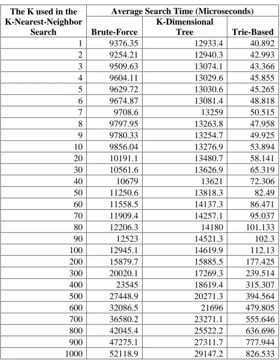
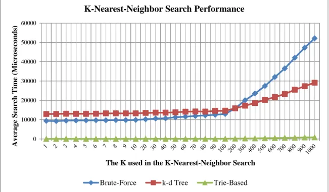
This thesis proposes a k-nearest-neighbor search method inspired by the grid space partitioning and the compact trie tree structure. A detailed implementation based on the Best-First-Nearest-Neighbor-Search scheme is presented and illustrated with sample data. Then k-nearest-neighbor search performance comparison is carried out among the proposed compact-trie-based method, the brute-force method, and the k-d tree based method, with one million two-dimensional spatial points and k up to 1000. The result of the comparison shows that the proposed method can perform up to 300 times better than the other two methods when k is small, suggesting that the proposed method might be suitable for low dimensions and location-dependent spatial queries in mobile computing.

v Acknowledgements

I greatly appreciate Dr. Wendy Osborn’s kindness, patience, tolerance, and help throughout my two years of struggle in pursuing my Master of Science degree in Computer Science at the Department of Mathematics and Computer Science, University of Lethbridge. I want to also thank my two committee members, Dr. Yllias Chali and Dr. John Zhang, for their valuable input and help. I am fortunate to have unconditional support from my beloved wife, Hui Sun, my parents, and my mother-in-law, as always. And I must thank you all very much for everyone who helped me and accompanied me so far. Last, I am indebted deeply to the Internet communities.

vi Contents

Abstract ... iv

Acknowledgements... v

Contents ... vi

List of Tables ... vii

List of Figures ... viii

Chapter 1 Introduction ... 1

1.1 Background ... 1

1.2 Contribution... 3

1.3 Thesis Outline... 3

Chapter 2 Background ... 5

2.1 Nearest Neighbor Search ... 5

2.2 Continuous Nearest Neighbor Search ... 13

2.3 Trie ... 19

2.4 Conclusions ... 25

Chapter 3 Compact-Trie-Based K-Nearest-Neighbor Search Method ... 26

3.1 Introduction ... 26

3.2 Step 1 Data Preparation ... 27

3.3 Step 2 Trie Construction... 30

3.4 Step 3 Query Search ... 41

3.5 Summary ... 42

Chapter 4 Evaluations ... 44

4.1 Implementation of Benchmark K-Nearest-Neighbor Search Methods ... 44

4.2 K-Nearest-Neighbor Search Performance Comparison ... 48

4.3 Summary ... 51

Chapter 5 Conclusion and Future Directions... 53

vii List of Tables

3.1 The Set of 15 Purposefully Designed Two-Dimensional Spatial Points ... 26 3.2 The Data Output Text Strings of the 15 Points ... 30 3.3 The Two-Dimensional Array Representation of the Compact Trie for

the 15 Points ... 34 3.4 The Brief Summary for Each Column of Table 3.3 ... 34 4.1 K-Nearest-Neighbor Search Performance Comparison ... 49

viii List of Figures

2.1 Nearest Neighbor Search and Conceptual Partitioning [28] ... 19

2.2 A trie for keys "A", "to", "tea", "ted", "ten", "i", "in", and "inn" [26] ... 20

2.3 An array-structured trie for bachelor, baby, badge, jar [14] ... 22

2.4 A list-structured trie for bachelor, baby, badge, jar [14] ... 24

3.1 The Compact Trie Constructed from the 15 Points ... 31

4.1 K-Nearest-Neighbor Search Performance Comparison Average Search Time ... 50

1

Chapter 1 Introduction

1.1 Background

Along with the popularity of smart phones and tablets is the rising of mobile computing. Location-aware-capable mobile devices demand location-dependent services. The location-dependent spatial query is one of such services and draws intensive research [33].

A spatial query is a special kind of database query supported by a spatial database. A spatial database is a database organized to store spatial data and optimized to facilitate spatial query processing. Spatial data, which represent objects in space, can be as simple as spatial points in arbitrary dimensions. For example, spatial data can be (Longitude, Latitude) pairs, representing points of interest on a two-dimensional map. All points of interest on the map can be organized in a spatial database, which is optimized to answer spatial queries such as which point of interest is closest to a given query point on the map [25].

A spatial query can be ad-hoc and terminated once the search result is returned. A spatial query can also be continuous if the query point is moving and the search result needs to be constantly updated in response to the latest known location of the query point, which is common in mobile computing. For example, one looks for the nearest gas station while driving. Location-dependent spatial queries refer to spatial queries of which the search result depends on the location of both the query point and spatial points stored in a spatial database. Continuous location-dependent spatial queries are common service

2

demanded by location-aware-capable mobile devices and pose great challenge on efficient spatial query processing [33].

Not only can a query point be moving, but also spatial points stored in a spatial database can be moving too, such as a spatial database of running taxis. It could require both the content and the organizational structure of the spatial database be updated constantly. The dynamic content and dynamic organizational structure ose great challenge on efficient spatial data organization in a spatial database [33].

In summary, because a query point can be static or mobile, and spatial points stored in a spatial database can also be static or mobile, a spatial query can involve (1) a static query point and a static spatial point database, (2) a static query point and a mobile spatial point database, (3) a mobile query point and a static spatial point database, or (4) a mobile query point and a mobile spatial point database. Furthermore, a spatial query can be ad-hoc or continuous. To illustrate, if a person stands still and looks for the nearest taxi while all taxis are parked, it is an ad-hoc spatial query involving a static query point and a static spatial point database; if the taxis start moving while the person remains standing still, it becomes a continuous spatial query involving a static query point and a mobile spatial point database; if the person starts moving while all taxis remain parked, it becomes a continuous spatial query involving a mobile query point and a static spatial point database; if both the person and the taxis start moving, it becomes a continuous spatial query involving a mobile query point and a mobile spatial point database.

Efficient spatial query processing at least depends on the kind of spatial query, the organization structure of the spatial database storing spatial data, and how a specific kind of a spatial query is processed.

3

Nearest neighbor spatial queries are one fundamental family of spatial queries important to many location-dependent services, such as in Geographic Information Systems. All aforementioned examples are nearest neighbor spatial queries. The core of nearest neighbor spatial queries, which is the nearest neighbor search, has applications far beyond spatial queries.

1.2 Contribution

A k-nearest-neighbor search method inspired by the grid space partitioning and the compact trie tree structure is proposed. Although the current implementation of the proposed method is limited to two-dimensional data, the result of k-nearest-neighbor search performance comparison shows significant improvement over the brute-force based and the k-d tree based k-nearest-neighbor search methods. Because most location-dependent mobile services rely on two-dimensional or three-dimensional geographic data, the proposed method might be particularly suitable for nearest neighbor based location-dependent spatial queries in mobile computing. Furthermore, the current implementation adopts a simple array-based data structure and an intuitive Best-First-Nearest-Neighbor-Search scheme.

1.3 Thesis Outline

The remainder of this thesis is organized as follows:

Chapter 2 Background knowledge of the thesis, continuous k-nearest-neighbor search and trie

4

Chapter 3 The detailed design and implementation of the proposed compact-trie-based k-nearest-neighbor search method for a set of 15 purposefully designed two-dimensional spatial points

Chapter 4 K-nearest-neighbor search performance comparison among the proposed compact-trie-based method, the brute-force based method, and the k-dimensional tree based method

5

Chapter 2 Background

2.1 Nearest Neighbor Search

In the era of “Big Data,” how to derive information from the “Big Data” more efficiently challenges and motivates us to develop better methods. Among them, nearest neighbor search methods are one important family drawing intensive research because they have wide applications and are foundational constituent for many methods [35]. Besides straightforward applications in spatial queries, nearest neighbor search has applications in areas such as pattern recognition, marketing, and multimedia information retrieval [35]. Nearest neighbor search is also frequently an integral part of clustering and classification methods [35].

Nearest neighbor search is firstly proposed by Minsky and Papert in 1969 [34]. It has also been referred to as the post office problem, proximity search, closest point search, and best match file searching problem [35].

The exact nearest neighbor search problem can be defined as: given a set of points P in an n-dimensional space S and a metric to determine the distance between any two points in S, how to most efficiently find the point in P which is nearest to an arbitrarily given query point q in S [34]. A generalization of nearest neighbor search is the k-nearest-neighbor search in which k points in P nearest to an arbitrarily given query point q in S are found, where k can be 1, 2, ... Another common variant of the nearest neighbor search is a range search, which finds all points in P in S that are within a pre-defined range of arbitrary shape and with respect to an arbitrarily given query point q in S.

6

The space S can be a metric space or a non-metric space. The nearest neighbor search in a non-metric space sometimes can be converted into a nearest neighbor search in metric space [35]. This thesis and the proposed methods here focus on the metric space and particularly on Euclidean space.

Ideally, an exact nearest neighbor or k exact nearest neighbors are being sought. In low dimensionality, an exact nearest neighbor search can be achieved in sub-linear or logarithmic time complexity [32]. However, the computational complexity of an exact nearest neighbor search can increase exponentially as the dimensionality increases. This phenomenon has been referred as the curse of dimensionality [1]. The efficiency of exact nearest neighbor search methods would degrade drastically as the dimensionality of space S increases [32].

However, if approximate nearest neighbors are being sought, the computational complexity even in high dimensionality could remain polynomial [20]. The approximate nearest neighbor search problem can be defined as: given a set of points P in n-dimensional space S and a metric to determine the distance between any two points in S, how to construct a data structure so that for an arbitrarily given query point q, it could most efficiently find all points whose distance to q is at most (1 + ε) times the distance from q to its nearest point in P, where ε is a positive number [20]. Locality-sensitive hashing, proposed by Piotr Indyk and Rajeev Motwani in 1998 [20], is one of the earliest approximate nearest neighbor search methods overcoming the curse of dimensionality and has received arguably the most attention in practical contexts [32].

This thesis and the proposed methods here focus on exact nearest neighbor search. I hope the work presented here can contribute in overcoming the curse of dimensionality for exact nearest neighbor search methods.

7

Many methods have been developed for the nearest neighbor search. Besides empirical analysis, the quality of those methods can be evaluated by the time complexity of the algorithm, and the space complexity of any data structure which must be maintained for the search [35]. So far, to the best of our knowledge, there is no universally applicable method which can obtain an exact solution to nearest neighbor search in arbitrarily high dimensional space with polynomial or polylogarithmic time complexity [32].

Based on whether any data structure must be maintained for the search, nearest neighbor search methods can be classified into structural-search and structureless-search. Structureless-search methods require that no data structure be purposefully maintained for the search. Structural-search methods improve the search time complexity at the expense of both the space complexity of the data structure(s) which must be maintained for the search, and the time complexity of preprocessing the data in order to obtain the data structure(s).

One structureless-search method and the most straightforward exact nearest neighbor search method is by brute-force, which first calculates the distance between the query point q and every point in the set of points P, then sorts all calculated distances, and last identifies the shortest distance(s) and the corresponding point(s) in P nearest to q. This method has a time complexity of O(nd) where n is the number of the points in the point set P and d is the dimensionality of the space S, and a space complexity of O(1) because no data structure is required to be maintained for the search. Weber et al. showed, from a theoretical perspective, that under the assumption that the data is uniformly distributed and all dimensions are independent from one another, an exact nearest neighbor search based on any partitioning scheme and clustering technique must

8

degenerate to a sequential scan through all data as dimensionality increases [36]. Therefore, this brute-force method provides a base benchmark.

Arguably, more nearest neighbor search methods are structural-search. As early as 1973, Burkhard and Keller proposed three file structures for nearest neighbor search, and the data structures are equivalent to multi-way trees [5]. In 1975, Fukunaga employed recursive decomposition of search space and applied branch-and-bound methodology to the resulting search data structure in nearest neighbor search [6]. The core of branch-and-bound methodology is that while systematically accessing and evaluating all candidate data, eliminate subset(s) of candidate data as early as possible and as much as possible according to the continuously optimized bound(s) derived during the evaluation. Recursive decomposition of search space is a recurring theme in space partition.

Also in 1975, Friedman et al. introduced the k-dimensional (k-d) tree which is

produced by recursively bisecting the search space with a hyperplane perpendicular to only one axis of the k dimensions [7]. A k-d tree is a binary tree where every non-terminal tree node has two and only two child nodes. It is constructed as follows. Strategically select a data point and a k-dimensional partition hyperplane that passes through the data point to divide the search space represented by the non-terminal node into two. The divided search space on one side of the hyperplane is represented by one of the two child nodes. The divided search space on the other side of the hyperplane is represented by the other of the two child nodes. The bisecting can be repeated at any non-terminal node in any level of the hierarchical tree as long as there is more than one data point in the search space represented by the non-terminal node.

The search time complexity of the k-d tree based method is improved to be logarithmic [8]. The k-d tree has also been applied to range search [9] and moderate

9

dimensions [10]. The hyperplanes and bisecting strategy can be chosen in a way to optimize the resulting k-d tree for a certain application [21].

Sproull proposed some ways to improve the k-d-tree-based nearest neighbor search. The measure of distance is assumed to be Euclidean. Because the Euclidean distance metric is invariant under rotation, Sproull proposed that the partition hyperplanes can be arbitrary k-dimensional hyperplanes [13], rather than requiring the partition hyperplanes be perpendicular to one coordinate axis as in the original algorithm proposed by Friedman et al [7]. However, as Sproull pointed out in the paper, an arbitrary partition

hyperplane is feasible but not always more favorable than a perpendicular partition hyperplane due to the additional cost of computing the distance between a point and the arbitrary partition hyperplane [13]. Choosing an arbitrary partition hyperplane perpendicular to an axis other than the coordinate axes could also incur additional costly computation [13].

Sproull’s method operates in a top-down fashion starting from the root node. At each non-terminal node, the search algorithm decides which one of its two child nodes need to be accessed next by identifying which divided search space represented by the child node encompasses the query point. Once the search reaches a terminal node, all data points within the search space represented by the terminal node will be examined exhaustively to find the nearest neighbor to the query point. However, the identified nearest neighbor must be verified by checking whether the true nearest neighbor could be on the other side of the partition hyperplane or the other divided search space, with respect to the current one. Sproull proposed that the check can be done by comparing the nearest distance identified so far with the distance between the query point and the partition hyperplane [13].

10

Arguably, the k-d tree based nearest neighbor search might be the oldest and most established one. The R-tree based spatial partitioning and spatial access methods, arguably, have received more applications in practice. Antonin Guttman proposed the R-tree in 1984 [11]. The R-R-tree is especially suitable for indexing multi-dimensional complex spatial data, such as polygons, because the key idea of R-tree is to group nearby spatial objects within a Minimum Bounding Rectangle (MBR) [11]. R in R-tree stands for Rectangle. The root node contains the MBRs of all spatial objects. A non-terminal parent node contains the MBRs of its immediate descendant nodes. A terminal node contains the MBRs of some spatial objects. If spatial data is organized into an R-tree, not only would the spatial relationship between the query point and MBRs be used to decide whether to search an MBR, and its descendant sub-trees, but also the k nearest neighbors can be efficiently computed via spatial join [15].

The key difficulties of the R-tree are how to efficiently build an R-tree from scratch, and how to best perform modification to an existing R-tree, such as insertion and deletion operations because MBRs may cover too much empty space and may overlap with one another too much. Most of the research and improvement for R-tree aim at conquering these key difficulties. Among them, the mqr-tree developed in this research group is a MBR based 2-dimensional spatial access method [30].

Numerous ways to partition search space or to index spatial data result in various hierarchical structures to facilitate nearest neighbor search. Two common branch-and-bound hierarchical search schemes are Depth-First Nearest Neighbor Search (DFNNS) and Best-First Nearest Neighbor Search (BFNNS) [24]. DFNNS can be traced back to Fukunaga’s 1975 paper [6]. DFNNS systematically visits every element of the hierarchical structure in a predetermined order. Starting from the root, it traverses as deep

11

as possible along every branch before backtracking, using the least qualified neighbor(s) found to prune branches and bound the search. BFNNS has been popular since the 1990s [16]. BFNNS starts from the root and then always visits the next best possible element by creating and maintaining a visit list sorted by probability.

Roussopoulos proposed a branch-and-bound tree traversal algorithm based on DFNNS for k-nearest-neighbor search and the algorithm can be applied to any tree-like data structure used for the purpose of indexing data [18]. A tree-like data structure generally has only two kinds of tree nodes: non-terminal nodes and terminal nodes. Only the terminal nodes store the data or references to the data, while the non-terminal nodes store the information of space partitions represented by the non-terminal nodes. A parent non-terminal node represents the space partition encompassing all space partitions represented by its child non-terminal nodes and/or data represented by its child terminal nodes. The root non-terminal node represents and encompasses the entire search space.

Two metrics are proposed and employed to help bound the search. One is the minimum distance (MINDIST) between the query point and the data point/object. The other is the minimum of the maximum possible distances (MINMAXDIST) from the query point to the space partition encompassing the data point/object. The search operates in a depth-first and top-down fashion starting from the root. If the node being accessed is a non-terminal node, then all of its child nodes will be sorted into an Active Branch List (ABL) by one of the two metrics, MINDIST or MINMAXDIST. If the node being accessed is a terminal node, then each data point/object represented in the terminal node will be evaluated to determine whether it is among the top k nearest neighbors to the query point. If it is, then it will be inserted into the result list according to its distance from the query point and the kth nearest distance will be updated accordingly. The

12

“branches” in the ABL will be constantly checked against one another by comparing their two metrics MINDIST and MINMAXDIST, as well as comparing against the most updated kth nearest distance. All unnecessary branches will be pruned. Then, the algorithm will be applied to the next remaining branch in the ABL recursively until the ABL becomes empty. The proposed pruning strategies are: (1) All branches whose MINDIST is larger than the kth nearest distance will be pruned; and (2) a branch whose MINDIST is larger than the MINMAXDIST of another branch will be pruned [18].

Hjaltason proposed an algorithm based on BFNNS suitable for the k-nearest-neighbor search and the value of k need not be known or fixed ahead of time because the search operates in an incremental fashion [19]. The algorithm can be applied to any hierarchical data structure representing the search space, such as a quadtree. In addition to the hierarchical data structure, the search employs a priority queue. The priority is determined based on the distance between the query point and a terminal node or the minimum distance between the query point and the space partition represented by a non-terminal node. If the minimum distance of a non-non-terminal node is equal to the distance of a terminal node, the search requires the non-terminal node take higher priority over the terminal node in the priority queue [19].

The search operates in a top-down fashion starting from the root as the only element of the priority queue, then recursively runs as follows. First, dequeue the first element of the priority queue. If the dequeued element is a terminal node, then append the data represented by the terminal node to the end of the result list, the furthest of nearest neighbors found so far. If the dequeued element is a non-terminal node, then insert all of its child nodes into the priority queue. The search stops when k nearest neighbors have been procured or when the priority queue becomes empty.

13

2.2 Continuous Nearest Neighbor Search

Compared to the ad-hoc nearest neighbor search methods, continuous nearest neighbor search methods can face some exclusive challenges, such as unknown velocity and trajectory of the moving query point, constrained moving path and even obstacles on the moving path. However, efficient spatial data indexing schemes, access methods, and search strategies continue to be the centerpieces of continuous nearest neighbor search methods. Thus, the continuous nearest neighbor search methods surveyed here focus on these centerpieces rather than those exclusive challenges.

In 2001, Song and Roussopoulos proposed a series of progressive methods to tackle the k-nearest-neighbor search for a moving query point [22]. The data points are assumed to be static, known beforehand and indexed by an R-tree-family structure. A static branch-and-bound R-tree-based depth-first k-nearest-neighbor-search algorithm is proposed to find the k nearest neighbors for a given location of the moving query point whenever necessary.

The location of the moving query point is determined by periodic sampling [22]. Therefore, a continuous k-nearest-neighbor query is transformed into queries to retrieve the k nearest neighbors of certain sampling points. The sampling may not address the need of certain applications, which expect that the k nearest neighbors are updated automatically and whenever necessary because the locations demanding update of k nearest neighbors may not be known in advance. The sampled locations largely depend on how the query point is moving without considering the static data points [22]. If the path of the moving query point is not known beforehand, sampling cannot be performed [22]. In this case, the “sampling” becomes a prediction based on current location and

14

velocity [22]. Therefore, the computed k nearest neighbors may not be an exact solution but an approximate solution. However, given that there is always some latency in communication, an exact solution to k-nearest-neighbor search might not be that necessary and an approximate solution is adequate.

The proposed progressive methods focus on maximizing the usage of the information obtained from the previous k-nearest-neighbor search and the distance between the current search position and the previous search position to at least eliminate unnecessary k-nearest-neighbor searches and to bound the search space [22]. One observation is that the kth shortest distance to current search location must be less than or equal to the sum of the kth shortest distance to the previous search location, and the distance between the current search location and the previous search location [22]. Another observation is that if n nearest neighbors, where n is larger than k, have already been computed, there is no need to perform another n nearest neighbor search if the distance between the current search location and the previous search location is less than or equal to the half of the difference between the nth and kth shortest distances to the previous search location [22]. Therefore, the proposed methods can provide a more bounded search space and reduce the frequency of needed k-nearest-neighbor searches. However, they perform better when the number of static data points is small, the query point moves slowly, and k is small [22].

In a method proposed by Tao in 2002, a continuous nearest neighbor query is defined as a query to retrieve k nearest neighbors of every point along a path q [23]. The query result is presented by pairing the k nearest neighbors with the corresponding path segment [23]. A series of “split” points are calculated along the path q. The starting point and the ending point of the path q constitute the first split point and the last split point,

15

respectively. Every path segment between two consecutive split points corresponds to a unique set of k nearest neighbors to that path segment [23].

In the proposed algorithm, given a known query path q and a continuous k-nearest-neighbor query, a k-k-nearest-neighbor query result is returned for every split path segment [23]. In terms of implementation, an R-tree is employed to index search space. Either a depth-first or best-first traversal paradigm can be adopted to prune the R-tree following the branch-and-bound methodology [23].

One limitation to the proposed algorithm is that the query path or trajectory must be known beforehand with the starting and ending points clearly defined. In addition, the path or trajectory seems to be composed of straight line segments only.

Instead of checking every point along the path q, only the split points need to be checked when evaluating a data point [23]. Initially, there are only two split points, the starting point and the ending point of the path q. By the definition of nearest neighbor, a data point must have the shortest distance to at least one already identified split point in order to be considered as a potential nearest neighbor [23]. Once a potential nearest neighbor is found, a new split point will be determined on the path q and the already identified set of split points may need adjustment, by eliminating some already identified split points and/or adding some new split points [23].

In 2005, Xiong proposed a general framework for processing a large number of simultaneous continuous k-nearest-neighbor (CKNN) queries [27]. The efficient concurrent processing is achieved by shared execution. All concurrent CKNN queries, along with their associated search regions, are grouped by similarity into a common query table [27]. Then, the problem of evaluating multiple CKNN queries is reduced to performing a spatial join between the query table and the object table [27]. Having a

16

shared execution reduces the number of scans needed over the object table, and therefore improves efficiency [27]. The output of the spatial join will be split and sent to the corresponding queries [27].

Xiong also proposed a way to efficiently process a CKNN query by incremental evaluation based on prior query results [27]. Any ad-hoc k-nearest-neighbor search algorithm can be utilized to obtain the set of k nearest neighbors whenever necessary [27]. The proposed method for CKNN search has no restrictions on the movement of the query and/or the objects. Both the query and the objects can move and nothing regarding their movement, such as velocity or trajectory, must be known beforehand. The incremental evaluation entails that only queries whose answers are affected by the movement of the objects and/or the query are reevaluated [27].

After an initial k-nearest-neighbor search, a CKNN query is associated with a circular search region, which is defined by the query as the center and the kth nearest distance to the query as the radius [27]. The incremental evaluation provides a minimum search region at next evaluation by taking the following three steps [27]:

1. Check if any objects that are originally outside the prior search region move into the prior search region, or if any objects originally inside the prior search region move within the prior search region. If there are such objects, the current search region will be set to the prior search region. Otherwise, no reevaluation is needed and the radius of the current search region would be set to 0.

2. Check if any objects originally inside the prior search region move out. If there are such objects, then the radius of the current search region will be set to the maximum distance between those objects and the prior query. Otherwise, the current search region inherits the result from Step 1.

17

3. If the query moves and if the radius of the current search region inherited from Step 2 is 0, then the radius of the current search region will be set to the sum of the radius of the prior search region and the distance the query travels. If the query moves and if the radius of the current search region inherited from Step 2 is not 0, then the radius of the current search region will be updated by adding the distance the query travels.

Also in 2005, Mouratidis proposed a way to tackle continuous k-nearest-neighbor queries by treating every query update as a new query with respect to the present location of the query and spatial objects [28]. The proposed method has no restrictions on the movement of the query and/or the spatial objects. Both the query and the spatial objects can move and nothing regarding their movement, such as velocity or trajectory, must be known beforehand.

The core k-nearest-neighbor-search proposed, conceptual partitioning [28], is illustrated in Figure 2.1 and elaborated as follows. First, the search space is partitioned as a grid consisting of uniform cells to group objects. Using two-dimensional Euclidean space as an example, as shown in Figure 2.1, conceptually partition the search space. An important observation is that the minimum distances of rectangles to the query point differ by δ for consecutive rectangles in the same direction (e.g. U0 and U1, R1 and R2, D2 and D3, and L0 and L1) [28]. Similar to the best-first nearest neighbor search, initially, the cell containing the query point and its immediately adjacent rectangles in all directions are inserted into an empty priority queue, which is sorted by their minimum distance to the query point [28]. Then, keep dequeuing the first element of the priority queue, which has the shortest minimum distance to the query point. If the dequeued element is a cell, then examine all objects in the cell to identify candidates for k nearest

18

neighbors and update the kth nearest distance accordingly. If the dequeued element is a rectangle, then insert all cells covered by the rectangle and the rectangle immediately adjacent to it that is outward and in the same direction into the priority queue according to their minimum distances to the query point [28]. Repeat until the minimum distance of the dequeued element to the query point is larger than the kth nearest distance, or the priority queue becomes empty. The proposed method does not address how to identify the cell containing the query point initially.

To address moving objects, the proposed method maintains cross reference tables for cells and queries [28]. What is kept include not only all prior search results, but also, for each query, all cells accessed in its prior search sorted by their minimum distance to the query point, and the remaining cells and rectangles in the priority queue at the end of its prior search [28]. Then, k-nearest-neighbor updates in response to moving objects can be evaluated with the aid of those additional information before a complete k-nearest-neighbor search is re-computed. Lastly, moving objects can be handled in a comprehensive way rather than independently [28].

19

Figure 2.1: Nearest Neighbor Search and Conceptual Partitioning [28]

Only four continuous nearest neighbor search methods are surveyed here, ranging from an approximation sampling method to an exact exhaustive method, and from a conceptual partition best-first ad-hoc search to a comprehensive orchestrated batch search. They serve to enlighten and inspire readers to come up with better methods for nearest neighbor search, k-nearest-neighbor search, continuous k-nearest-neighbor search, and simultaneous multiple continuous k-nearest-neighbor queries.

2.3 Trie

In computer science, the trie, also referred to as a prefix tree, is one kind of digital search tree [4]. The term “trie” was coined by Edward Fredkin and abbreviated from “retrieval” [2]. So, since day one, trie has been associated with information retrieval.

As its other common name “prefix tree” indicates, trie is a tree data structure and strongly associated with the prefix of strings. The root node of a trie is associated with an empty string and all immediate descendants of any one trie node have a common prefix

20

string which would be associated with that trie node. As illustrated in Figure 2.2, a trie can be an effective and efficient data structure for indexing strings. Strings are indexed in a hierarchical structure according to their common prefixes and in an ascending order of the length of their common prefixes. Every unique leaf (or terminal) node of a trie uniquely corresponds to a unique string; and every unique string is uniquely represented by a unique leaf node. Therefore, there is a one-to-one mapping between unique strings and terminal trie nodes. Compared to imperfect hash-based indexing methods, there is no “conflict” in trie indexing.

Figure 2.2: A trie for keys "A", "to", "tea", "ted", "ten", "i", "in", and "inn" [26]

Searching a string within a trie is by traversing trie nodes starting from the root node. The trie node to be traversed next is determined by a match of the prefix of the

21

query string with the string associated with the trie node. The search would terminate at the trie node whose associated string is the longest common prefix among the query string and all strings indexed by the trie. Therefore, the time complexity of the search operation is bound by O(k) where k is the maximum length of all strings indexed by the trie. So are the insertion and deletion operations because before inserting or deleting a string, a search of the string within the trie must be completed first. Only if the string is found within the trie, a deletion can be completed. Also, only if the string cannot be found within the trie, an insertion can be completed. Furthermore, the search provides where exactly to insert or delete the string.

A compact trie is a space-optimized trie, which is organized by requiring all non-terminal trie nodes to have more than one descendant [3]. The time complexity of search operation within a compact trie is also bound by O(k), but is likely, on average, less than its equivalent full trie because the compact trie would likely have fewer non-terminal nodes than its equivalent full trie and searching within fewer non-terminal nodes would on average take less time. Although insertion and deletion operations within a compact trie can involve adding, splitting, and merging branches, as well as other additional operations, besides search operation, the time complexity of insertion and deletion operations within a compact trie remains to be bound by O(k). And insertion and deletion operations are not always needed as in a read-only static trie.

The most naïve implementation of a trie is as illustrated in Figure 2.3. Each trie node is an array of pointers. The number of pointers in the array is the number of possible characters in the strings indexed by the trie. The pointer would point to a descendant trie node. If all pointers in the array are null pointers, the trie node is a terminal leaf node. As illustrated in Figure 2.3, even in non-terminal trie nodes, most pointers are null pointers.

22

Therefore, not only the space complexity of this naïve implementation is proportional to the product of the number of trie nodes and the number of possible characters, but also the space wasted by null pointers could be extravagant, which is especially true when the trie is sparse.

Figure 2.3: An array-structured trie for bachelor, baby, badge, jar [14]

The arrays of pointers can be replaced by linked lists as illustrated by Figure 2.4. In this implementation, every non-null pointer in the naïve implementation is represented by a structure containing three elements: “arc label,” “next node,” and “other label.” “arc

23

label” signifies which character a non-null pointer stands for. “next node” points to the first non-null pointer of the immediate descendant trie node, if any, or would be null (nil) if there is no descendant trie node. “other label” points to the next non-null pointer in the same trie node, if any, or would be null (nil) if there is no more non-null pointer in the same trie node. A terminal trie node would have both “next node” and “other label” as null (nil). The space complexity of this linked-list implementation could be much less than its equivalent naïve implementation because this linked-list implementation wastes no space on null pointers as its equivalent naïve implementation. However, due to the linear search in a trie node for a particular non-null pointer, which, in the worse scenario, could have to access all non-null pointers in the trie node, the time complexity of search operation in this linked-list implementation of trie cannot be bound by O(k). Thus, the improvement on the space complexity of this linked-list implementation is at the expense of the time complexity.

24

Figure 2.4: A list-structured trie for bachelor, baby, badge, jar [14]

Naturally, it would be ideal if an implementation of trie could preserve the time complexity of the naïve implementation and the space complexity of the linked-list implementation. In 1989, Jun-Ichi Aoe proposed the double-array implementation of trie which can guarantee the time complexity of search operation to be bound by O(k) and reduce the space complexity from the product of the number of possible characters and the number of trie nodes to their sum [12]. As its name indicates, in double-array implementation, a trie is represented by two arrays, namely BASE and CHECK. Constructing a double-array trie and performing basic operations within the double-array

25

trie, such as search, insertion, and deletion, must all conform the following rule: traversing from a parent trie node S to its immediate child trie node T because of character C must satisfy T = BASE[S] + CODE[C] and CHECK[T] = S. CODE[C] represents a unique numerical code for character C. All trie nodes are mapped to the indexes of BASE and CHECK. Special algorithms are developed to construct a double-array trie and perform basic operations within the double-double-array trie according to the rule. Various improvements to this double-array implementation of trie have been developed to make the implementation more compact [31], space-efficient [17] and cache-conscious [29].

2.4 Conclusions

Inspired by the trie, its guaranteed search, insertion, and deletion performance in constant time regardless the size of the data indexed by trie, its zero conflict in indexing data, its compact, space-efficient, cache-conscious, array implementation, I developed a method based on array-implemented trie to facilitate space partition and nearest neighbor search suitable for low dimensions and location-dependent spatial queries in mobile computing.

26

Chapter 3 Compact-Trie-Based K-Nearest-Neighbor Search Method

3.1 Introduction

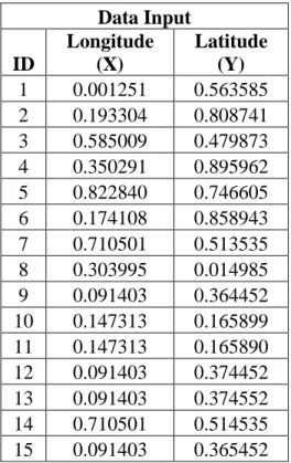
In this chapter, a compact-trie-based k-nearest-neighbor search method is proposed. The method can be divided into three steps: (1) data preparation, (2) trie construction, and (3) query search. Inspired by the (Longitude, Latitude) pair of Global Position System (GPS) data format, such as (47.644548, -122.326897), I designed a set of 15 two-dimensional spatial points whose coordinates are positive pure decimal numbers, as listed in Table 3.1, to illustrate the proposed method in detail. The number of digits after the decimal point is 6 in the present illustration and can be larger if higher spatial resolution is needed for the application.

Table 3.1: The Set of 15 Purposefully Designed Two-Dimensional Spatial Points Data Input ID Longitude (X) Latitude (Y) 1 0.001251 0.563585 2 0.193304 0.808741 3 0.585009 0.479873 4 0.350291 0.895962 5 0.822840 0.746605 6 0.174108 0.858943 7 0.710501 0.513535 8 0.303995 0.014985 9 0.091403 0.364452 10 0.147313 0.165899 11 0.147313 0.165890 12 0.091403 0.374452 13 0.091403 0.374552 14 0.710501 0.514535 15 0.091403 0.365452

27

As shown in Table 3.1, each two-dimensional spatial point is given a unique ID which is an integer ranging from 1 to 15 (in the first or the leftmost column). And each two-dimensional spatial point is composed of Longitude (X) (in the second or the middle column) and Latitude (Y) (in the third or the rightmost column) coordinates. The coordinates are positive pure decimal numbers with 6 digits after the decimal point for simplicity and uniformity. These positive pure decimal numbers were purposefully designed to make the compact trie constructed based on them more generic or representative.

3.2 Step 1 Data Preparation

All spatial points are assumed unique. Therefore, a set of spatial points should be preprocessed firstly to remove duplicate point(s), if any.

Secondly, all coordinate numbers shall be normalized to positive pure decimal numbers between 0 and 1. The normalization can be achieved by first determining the maximum number of digits before the decimal point among all coordinate numbers, and then dividing all coordinate numbers uniformly by ten to the power of this maximum number. If the only digit before the decimal point is 0, then the maximum number of digits before the decimal point is deemed to be 0, rather than 1; if the only digit before the decimal point is not 0, then the maximum number of digits before the decimal point is deemed to be 1. For example, a series of four positive decimal numbers (2.3, 1, 0.835, 12) can be normalized to (0.023, 0.01, 0.00835, 0.12) by dividing all four numbers by ten to the power of 2 or 100 because the maximum number of digits before the decimal point among all four numbers is 2.

28

Thirdly, determine the maximum number of digits after the decimal point among all normalized positive pure decimal numbers, and then make all normalized positive pure decimal numbers to have the same maximum number of digits after the decimal point by appending trailing zero(s) if necessary. For example, a series of four positive decimal numbers (2.3, 1, 0.835, 12) can be eventually transformed to (0.02300, 0.01000, 0.00835, 0.12000), all of which have 5 digits after the decimal point. The goal of such transformation so far is to make all positive decimal numbers to become positive pure decimal numbers of equal length before further processing. The spatial distance relationship among every pair of points should be preserved after such transformation because all coordinate numbers are uniformly scaled down.

Fourthly, the core of Step 1 Data Preparation is to, for each spatial point, assemble a string composed of digits only, based on its preprocessed positive pure decimal number coordinates, by interleaving the digits after the decimal point of all coordinates in an orderly fashion. The complete numeric information of the multi-dimensional coordinates of the spatial point will be preserved. Take spatial point 1 (0.001251, 0.563585) from Table 3.1 for example to illustrate the assembling process. The first digits after the decimal point of the two coordinates are 0 and 5. Interleave them to form a string “05”. Next, the second digits after the decimal point of the two coordinates are 0 and 6. Interleave them in the same order to form a string “06”. Append the string “06” to the string “05” to form a string “0506”. Repeat the same interleaving and appending procedures for the third, fourth, fifth, and last digits after the decimal point of the two coordinates, ultimately resulting in the final string “050613255815” for spatial point 1 (0.001251, 0.563585). Data processing or preparation so far would result in the same

29

number of strings as the number of unique spatial points. All strings are equal in length. Each string corresponds to one unique multi-dimensional spatial point.

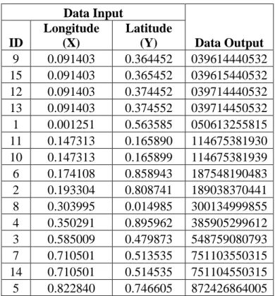
Lastly, the equal-length strings are output in an ascending order according to their numeric values, had they been converted to integers, along with their corresponding spatial points. Such an ordered output naturally groups together strings sharing the longest common prefix, as illustrated in Table 3.2 “Data Output” column. For example, “039614440532” and “039615440532” are grouped together because they share the common prefix “03961”; “039714440532” and “039714450532” are grouped together because they share the common prefix “0397144”; “039614440532”, “039615440532”, “039714440532” and “039714450532” are grouped together because they share the common prefix “039”; “114675381930” and “114675381939” are grouped together because they share the common prefix “11467538193”; “187548190483” and “189038370441” are grouped together because they share the common prefix “18”; and “751103550315” and “751104550315” are grouped together because they share the common prefix “75110”. They also illustrate my intention to make the compact trie constructed based on these data more generic and representative. The purpose of such an ordered output is to facilitate the compact trie construction in Step 2. It is worth mentioning that sorting strings in some way is frequently employed in the initial construction of a trie out of a large number of strings.

Table 3.2 below presents the final “Data Output” of strings after Step 1 Data Preparation based on the “Data Input” of spatial points. These strings will be the input for Step 2 Trie Construction.

30

Table 3.2: The Data Output Text Strings of the 15 Points Data Input Data Output ID Longitude (X) Latitude (Y) 9 0.091403 0.364452 039614440532 15 0.091403 0.365452 039615440532 12 0.091403 0.374452 039714440532 13 0.091403 0.374552 039714450532 1 0.001251 0.563585 050613255815 11 0.147313 0.165890 114675381930 10 0.147313 0.165899 114675381939 6 0.174108 0.858943 187548190483 2 0.193304 0.808741 189038370441 8 0.303995 0.014985 300134999855 4 0.350291 0.895962 385905299612 3 0.585009 0.479873 548759080793 7 0.710501 0.513535 751103550315 14 0.710501 0.514535 751104550315 5 0.822840 0.746605 872426864005

In terms of implementation, standard built-in string operators and functions can be used to assemble the output strings. To guarantee performance, standard built-in sorting functions can be employed to output the strings orderly.

3.3 Step 2 Trie Construction

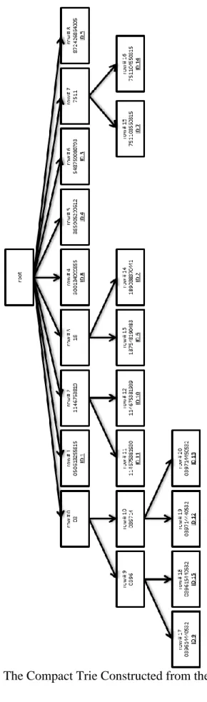
In this proposed compact-trie-based k-nearest-neighbor search method, the compact trie is constructed from multi-dimensional spatial points (or data) via their corresponding strings, for the purpose of indexing and accessing the spatial points (or data) effectively and efficiently. The compact trie that is constructed from the strings in Table 3.2 Column “Data Output” above is shown in Figure 3.1 below.

31

32

As shown in Figure 3.1, the compact trie constructed from the set of 15 purposefully designed two-dimensional spatial points is composed of a total of 22 nodes, each of which is represented by a rectangular box. There is always one and only one depth-0 node, the root node, which is associated with an empty string according to the definition of the trie. In this proposed method, every other node of the compact trie is associated with one unique string. The unique string associated with any non-terminal node (except for the root node) is the longest common prefix of all strings associated with its immediate child nodes and the length of this longest common prefix must be an integral multiple of the dimensionality of the spatial points. (The rationale behind such a length will be elaborated upon later.) Every terminal node is associated with one unique string corresponding to one unique spatial point. Therefore, there are 15 terminal nodes in total. Every rectangular box, except for the one representing the root node, contains the unique string associated with the node represented by the rectangular box, as well as one unique “row #” indicating which row of a two-dimensional array, as shown in Table 3.3, stores the information of that node. The detail of this two-dimensional array will be elaborated upon shortly. The rectangular box representing a terminal node also contains the unique “ID” associated with the spatial point uniquely corresponding to that terminal node.

With respect to the arrows in Figure 3.1, an arrow in the compact trie points from a parent node to its immediate child node. The directional arrow is not intended to suggest that the traverse between a parent node and its immediate child node is only in one direction. The directional arrow is used to indicate the parental-child relationship between the two nodes. The traverse between a parent node and its immediate child node is bi-directional. In other words, a tree traversing program would be able to traverse either

33

from a parent node to its immediate child node or from a child node to its immediate parent node. A node can be accessed both from its immediate parent node and from its immediate child node, if they do exist.

If there is no arrow between two nodes, accessing one node from the other node must be via existing arrows or paths. For example, accessing node Row #0 from node Row #9 can be achieved directly from node Row #9, and vice versa, because there is an arrow or a path between node Row #0 and node Row #9. However, because there is no arrow or path between node Row #0 and node Row #11, accessing node Row #0 from node Row #11 must be via at least the path between node Row #11 and node Row #2, then the path between node Row #2 and the root node, and last the path between the root node and node Row #0, and vice versa.

In terms of implementation, such a bi-directional traverse can be achieved by requiring the information of any node to include pointers to its immediate parent node and all of its immediate child nodes. Any node, except for the root node, must have one and only one immediate parent node. Any non-terminal node of the compact trie must have more than one immediate child node according to the definition of the compact trie. All terminal nodes do not have any child nodes and the root node does not have a parent node.

34

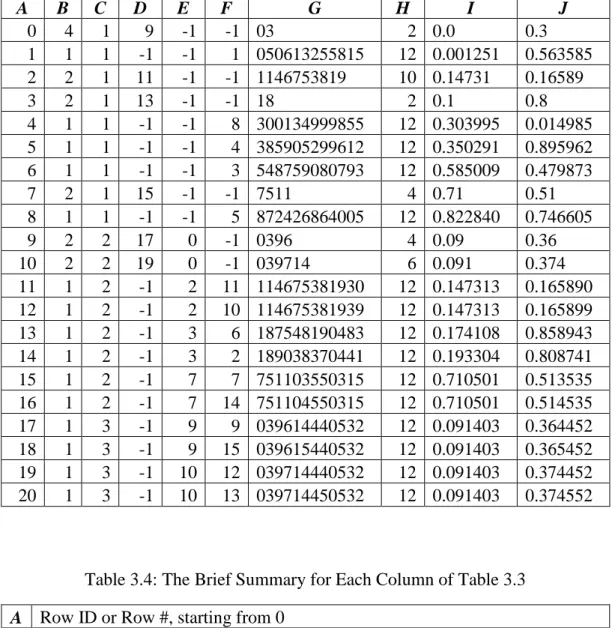
Table 3.3: The Two-Dimensional Array Representation of the Compact Trie for the 15 Points A B C D E F G H I J 0 4 1 9 -1 -1 03 2 0.0 0.3 1 1 1 -1 -1 1 050613255815 12 0.001251 0.563585 2 2 1 11 -1 -1 1146753819 10 0.14731 0.16589 3 2 1 13 -1 -1 18 2 0.1 0.8 4 1 1 -1 -1 8 300134999855 12 0.303995 0.014985 5 1 1 -1 -1 4 385905299612 12 0.350291 0.895962 6 1 1 -1 -1 3 548759080793 12 0.585009 0.479873 7 2 1 15 -1 -1 7511 4 0.71 0.51 8 1 1 -1 -1 5 872426864005 12 0.822840 0.746605 9 2 2 17 0 -1 0396 4 0.09 0.36 10 2 2 19 0 -1 039714 6 0.091 0.374 11 1 2 -1 2 11 114675381930 12 0.147313 0.165890 12 1 2 -1 2 10 114675381939 12 0.147313 0.165899 13 1 2 -1 3 6 187548190483 12 0.174108 0.858943 14 1 2 -1 3 2 189038370441 12 0.193304 0.808741 15 1 2 -1 7 7 751103550315 12 0.710501 0.513535 16 1 2 -1 7 14 751104550315 12 0.710501 0.514535 17 1 3 -1 9 9 039614440532 12 0.091403 0.364452 18 1 3 -1 9 15 039615440532 12 0.091403 0.365452 19 1 3 -1 10 12 039714440532 12 0.091403 0.374452 20 1 3 -1 10 13 039714450532 12 0.091403 0.374552

Table 3.4: The Brief Summary for Each Column of Table 3.3

A Row ID or Row #, starting from 0

B The number of terminal nodes among itself and its child nodes

C The depth or level of a node

D

The Row # of the first row of consecutive rows occupied by the node's immediate child nodes, if any

E

The Row # of the node's immediate parent node, or -1 if the node's immediate parent node is the root node

F

The ID of the spatial point associated with the node if it is a terminal node, or -1 if it is not

G The unique string associated with the node

H The length of the unique string associated with the node

I The restored X Cartesian coordinate

35

The compact trie in Figure 3.1 can be represented by a simple two-dimension array as shown in Table 3.3. Each column of Table 3.3 (A - J) represents a different attribute of the compact trie node. A brief summary for each column is provided for in Table 3.4.

This array representation of the compact trie is inspired by the double-array trie implementation which implements a trie by two parallel arrays [12]. However, the double-array trie implementation was not adopted because not all trie operations, such as the insertion and deletion of nodes, are needed in this proposed method.

It is worth mentioning that not every column in Table 3.3 is essential to the nearest-neighbor search. Exactly which column or what attribute is essential to the k-nearest-neighbor search depends on the k-k-nearest-neighbor search algorithm and its implementation. For example, for this proposed method, only columns D, E, I and J are necessary. All the other columns in Table 3.3 are presented for the purpose of better illustrating the method. The content and especially the order of rows in Table 3.3 dictate the compact trie construction program which takes Table 3.2 as input and outputs Table 3.3.

In Table 3.3, each row of the two-dimensional array represents one unique compact trie node in Figure 3.1, except for the root node. That is why there are only 21 rows in total, rather than 22, the number of nodes in Figure 3.1. For example, the first row represents node Row #0.

Column A is the row ID or Row #. The first row ID or Row # is 0 due to the convention of programming.

Column B is set to 1 if the node is a terminal node. If the node is not a terminal node, Column B is set to the number of its terminal child nodes, which might not be its

36

immediate child nodes. For example, the first row Column B is 4 because node Row #0 has 4 terminal child nodes: node Row #17, node Row #18, node Row #19, and node Row #20, as seen in Figure 3.1.

Column C is the depth or level of a node and the root node is the only node of depth 0. For example, the first row Column C is 1 or depth 1, as seen in Figure 3.1.

Column D is set to -1 if the node is a terminal node. If the node is not a terminal node, Column D is set to the Row # of the first row of consecutive rows occupied by its immediate child nodes. For example, the first row Column D is 9 because node Row #0 has two immediate child nodes, node Row #9 and node Row #10, which occupy the consecutive rows Row #9 and Row #10, and the first row of those consecutive rows is Row #9.

Column E is the Row # of the node’s immediate parent node, or set to -1 if the node’s immediate parent node is the root node. For example, the first row Column E is -1 because node Row #0’s immediate parent node is the root node, as seen in Figure 3.1.

Column F is set to -1 if the node is not a terminal node. If the node is a terminal node, Column F is set to the unique ID of the spatial point associated with the terminal node. For example, the first row Column F is -1 because node Row #0 is not a terminal node.

Column G is the unique string associated with the node. For example, the first row Column G is “03” because the unique string associated with node Row #0 is “03”.

Column H is the length of the unique string associate with the node. For example, the first row Column H is 2 because the length of the unique string “03” associated with node Row #0 is 2.

37

Column I and Column J are the X and Y Cartesian coordinates restored from the unique string associated with the node by reversing the assembling process in Step 1 Data Preparation. For example, node Row #20 is a terminal node, the unique string associated with it is “039714450532”, the ID of the spatial point associated with it is 13, and the X and Y Cartesian coordinates of spatial point 13 are 0.091403 and 0.374552, which are restored in Row #20 Column I and Column J, respectively. The first row Column I and Column J are 0.0 and 0.3, respectively, which are restored from the unique string “03” associated with node Row #0 by reversing the assembling process.

Last, I would like to connect all dots and elaborate on the rationale behind this proposed compact-trie-based k-nearest-neighbor search method. The method is inspired by the intrinsic relationship between grid partitioning and the Cartesian coordinates composed of positive pure decimal numbers.

Partitioning an n-dimensional space by orthogonal lines into n-dimensional grids is an intuitive space partitioning method. Take a simple square-shaped two-dimensional space for example to illustrate grid partitioning. Applying the Cartesian coordinate system, the original space before any grid partitioning can be defined by the Cartesian coordinates of its four corners counterclockwise: the lower-left corner (0, 0), the lower-right corner (1, 0), the upper-right corner (1, 1), and the upper-left corner (0, 1). Further, the original space can be denoted or labeled by the Cartesian coordinates of its lower-left corner (0, 0). Then partition the original space into 10 by 10, 100 square-shaped, non-overlapping regions evenly by orthogonal lines. Each region can be denoted or labeled by the Cartesian coordinates of its lower-left corner, such as (0.0, 0.0), (0.0, 0.1), (0.0, 0.2) … (0.9, 0.9). Any one region, such as the one labeled as (0.2, 0.3), can be partitioned further into 10 by 10, 100 square-shaped, non-overlapping sub-regions evenly by orthogonal

38

lines. Each sub-region can be denoted or labeled by the Cartesian coordinates of its lower-left corner, such as (0.20, 0.30), (0.20, 0.31), (0.20, 0.32) … (0.29, 0.39). Such recursive partitioning of a space can be performed infinitely. The resulting space region can be infinitely small so as to be deemed as a spatial point. Alternatively, any spatial point can be deemed as a certain space region. For example, the spatial point (0.20, 0.31) can be deemed as the space region labeled as (0.20, 0.31). So the Cartesian coordinates of a spatial point composed of positive pure decimal numbers can be deemed as the label of a certain space region resulted from such a grid partitioning.

The labels of space regions at the same partitioning level and different partitioning levels can be organized into a hierarchical structure by making some modifications to the labels as follows. Continuing with the grid partitioning example, the labels of the space regions at the first level of partitioning: (0.0, 0.0), (0.0, 0.1), (0.0, 0.2), …, (0.9, 0.9) can be modified by removing the leading “0.” and then combining the remaining digits of all coordinates to become 00, 01, 02, …, 99. Similarly, the labels of the space regions at the second level of partitioning: (0.20, 0.30), (0.20, 0.31), (0.20, 0.32), …, (0.29, 0.39) can be modified to become 2300, 2301, 2302 … 2399 (interleaving the remaining digits of all coordinates in an orderly fashion rather than simply combining them together). The common prefix “23” is the label of the first level space region encompassing the 100 second level space sub-regions which can be uniquely denoted by the rest suffixes “00”, “01”, “02”, …, “99”, respectively. Similar modifications can be applied to any space region at any level of partitioning.

Here are some benefit resulted from such modifications. The new labels are more succinct. New labels different in length suggest their corresponding space regions are at different levels of partitioning. The longer a new label is, the higher the partitioning level

39

of the corresponding space region is and the smaller the corresponding space region is. New labels equal in length suggest their corresponding space regions are at the same level of partitioning. New labels sharing a common prefix are within the same space region of which the new label is the common prefix. Last, such modifications explain how and why the Cartesian coordinates of spatial points composed of positive pure decimal numbers are assembled into the strings in Step 1 Data Preparation.

The grid partitioning described earlier would not result any partially overlapped space regions. Space regions at the same level of partitioning are non-overlapping. A space region at a lower level of partitioning would either encompass a space region at a higher level of partitioning or not. A tree-type data structure is naturally fit for organizing the space regions resulted from such a grid partitioning. The root node can represent the entire space. Every other node can represent a certain space region. The level of a node can indicate the partitioning level of the space region represented by the node. There is no direct connection between any pair of nodes at the same level. The direct connection between an upper level node and a lower level node can indicate the space region represented by the upper level node encompasses the space region represented by the lower level node.

The compact trie is adopted to store, index, and search spatial points. The spatial points can be deemed as space regions resulted from the grid partitioning described earlier. Every node of the compact trie represents a certain space region and is associated with the new label of the space region. The new label associated with any non-terminal node, except for the root node, must be the longest possible common prefix of the new labels associated with its immediate child nodes, and the length of the common prefix must be an integral multiple of the dimensionality of the spatial points. The space region