Blind audio source counting and separation of anechoic mixtures using the multichannel complex NMF framework

(1)

Blind audio source counting and separation of anechoic

mixtures using the multichannel complex NMF framework

Sayeh Mirzaei

a,n

, Hugo Van hamme

a

, Yaser Norouzi

b

a

Department of Electrical Engineering, KULeuven, Belgium

b

Department of Electrical Engineering, Amirkabir University, Tehran, Iran

a r t i c l e i n f o

Article history:

Received 24 November 2014 Received in revised form 28 January 2015 Accepted 8 March 2015 Available online 18 March 2015 Keywords:

Blind Source Separation (BSS)

Complex Non-negative Matrix Factorization (CNMF)

Binary masking Anechoic mixture

a b s t r a c t

In this paper, we address the tasks of audio source counting and separation for a stereo anechoic mixture of audio signals. This will be achieved in two stages. In the first stage, a novel approach is introduced for estimating the number of sources as well as the channel mixing coefficients. For this purpose, a 2-D spectrum is evaluated against both the phase and amplitude differences of the two channels. Hence, obtaining the peak locations of the spectrum yields the number of the sources and the corresponding channel coefficients. In the second stage, an extension of a single channel complex matrix factorization method to multichannel is developed to extract the individual source signals. We find primary estimates of the sources via binary masking and then apply the complex factorization to the complex spectrogram of each source. The obtained factors are then utilized as initial values in the complex multichannel factorization model. We also suggest a method for estimating the number of required components for modeling each source. The separation performance improvement over the conventional methods is investigated by calculating BSS evaluation metrics. The comparison is also carried out in terms of source counting and localization with the recently proposed DeMIX-Anechoic method.

&2015 The Authors. Published by Elsevier B.V. This is an open access article under the CC BY-NC-ND license (http://creativecommons.org/licenses/by-nc-nd/4.0/).

1. Introduction

Most audio signals are mixtures of several sources which might be active concurrently. Separation of audio signals is required for several audio processing tasks such as speech recognition, speaker identification, and poly-phonic music transcription.

When no prior information of the sources or channel mixing system is available, the task is called Blind Source Separation (BSS). When the mixing coefficients are real value gains, the mixture is termed instantaneous. However in real environments, the mixing process consists of a

linear time-invariant filtering of the source signals as

xiðtÞ ¼ XJ j¼1 X1 τ¼ 1 aijð

τ

Þsjðt

τ

Þ; i¼1;2 ð1Þ where sjðtÞ, j¼1…J, are the source signals and aijð

τ

Þ denotes the mixing filter. If the length of the filters aij are sufficiently smaller than the window length,(1)can be represented in the frequency domain as the following approximation:

Xft¼AðfÞSft ð2Þ

whereXft¼ ½X1ftX2ftT indicates the mixture signal com-plex STFT coefficients on two channels.AðfÞrepresents the 2J matrix containing the channel mixing coefficients and Sft¼ ½S1ft…SJftT denotes the complex spectrogram coefficients of the sources. For the case of anechoic mix-tures where no reflection is assumed from the objects

Contents lists available atScienceDirect

journal homepage:www.elsevier.com/locate/sigpro

Signal Processing

http://dx.doi.org/10.1016/j.sigpro.2015.03.006

0165-1684/&2015 The Authors. Published by Elsevier B.V. This is an open access article under the CC BY-NC-ND license (http://creativecommons.org/licenses/by-nc-nd/4.0/).

n_{Corresponding author.}

(2)

existing in the environment, the complex valued coeffi-cients of matrix A have frequency independent magni-tudes while their phase varies with frequency depending on the microphone array arrangement and the source location w.r.t. the array. The Fourier transform of the mixing filter coefficients can be parameterized as[12]

aijð Þ ¼f

κ

ijei2πfτij

κ

ij¼ 1 ffiffiffiffiffiffi 4

π

p rij and

τ

ij¼ rij Cs ð3Þ

whererijspecifies the distance betweenjth source andith microphone andCsis the sound propagation velocity.

In a more realistic environment, there are several paths besides the direct path from which the signals impinge on the microphones. The mixtures of this scenario are called convolutive and the A coefficients cannot be assumed frequency independent anymore in this case.

In this paper, we propose a framework for anechoic mixtures but we also apply it to the mixtures in moderate reverberant environments. We confirm the effectiveness of the model even in the presence of multipath propagation. Many methods have been developed for blind source separation. They either work based on a known channel mixing system or they try to estimate the mixing system in advance. Most of the channel mixing estimation techni-ques are based on time difference of arrival (TDOA) estimation in every time–frequency (TF) cell of the STFT representation of the mixture which is followed by clus-tering of the obtained estimates[1]. In Yilmaz and Rickard [32], Winter et al. [31], and Saab et al.[22], a clustering algorithm is used for finding the clusters around the actual mixing vectors. Besides some drawbacks associated to the spatial aliasing issue, most of these approaches suffer from an important deficiency which is the need that the number of clusters or sources be known in advance. Moreover, the assumption of strong sparsity is an essential requirement of most of these methods. It means that there should be only one dominant active source in each TF cell of the mixture STFT representation. However, the sparsity can be violated either in the presence of noise or when the sources overlap.

Due to the above mentioned disadvantages, we do not opt for clustering based methods. Instead, we obtain a 2-D spectrum against the amplitude and phase differences of the two channels as described in Section 2. The peak locations of this spectrum correspond to the mixing coefficients. This way, we have relaxed the above men-tioned sparsity assumption in the sense that we require a sufficient number of sparse TF cells for acquiring clear spectrum peaks corresponding to each source.

Independent Component Analysis (ICA) is a well-known BSS approach. Generally, ICA assumes that source signals are independent and it involves the so-called permutation problem since ICA is applied to separate frequency cells of the STFT representation. Hence, the source orders should be determined per frequency. This issue has been considered and solved in[13,23,19,25]. But ICA is just applicable to over-determined problems where the number of sensors is at least as large as the number of the sources. Under-determined mixtures are more often

separated using TF masking techniques[32,21]or classical sparse approaches such as l1-norm [6] or lp-norm [27] minimization.

Recently, Non-negative Matrix Factorization (NMF) has been applied extensively to several source separation scenarios in a single channel [26,14,30,8,5] and multi-channel[20,10,11,18]setting. NMF or Non-negative Tensor Factorization (NTF) is generally applied to the magnitude spectrogram domains. One of the shortcomings of these structures is that they disregard the phase information of the signal in the sense that they try to approximate the power or magnitude spectrogram of the mixture signal as a product of two non-negative matrices containing spec-tral components and time activations. Moreover, the number of the sources as well as components modeling each source should be known in advance.

In Kameoka et al. [15], a complex NMF model is introduced defining a mixing model in the complex-spectrogram domain. This model is able to provide a sparse representation of acoustic signals in a single-channel scenario. Utilizing this framework for the source separation task, we still need to know the model order in terms of the number of the sources and the components required for modeling each source.

In our present work, we have extended the method in Kameoka et al.[15]to the multichannel case. Our method differs from that of Sawada et al.[24,4]in the sense that they have proposed techniques for source separation in reverberant environment based on modeling the spatial covariance matrix. In Arberet et al.[4], the contribution of each source to the mixture channels in the time–frequency domain is modeled by a zero-mean Gaussian random vector with a full rank covariance matrix composed of two terms: a variance which represents the spectral properties of the source and which is modeled by a non-negative matrix factorization model and another full rank covariance matrix which encodes the spatial properties of the source contribution in the mixture. The extended

complex NMF model in Sawada et al. [24] has been

developed to factorize the covariance matrix and the spatial property is associated with each NMF basis. How-ever our proposed method is directly applied to the complex spectrogram of the mixture signal, thus it involves less computation. The estimates of the number of the sources and channel mixing given by the previous stage are exploited as known parameters in our developed model. A primary estimate of each source complex spec-trogram is obtained through binary masking. Then, the complex NMF approach proposed in Kameoka et al.[15]is applied for decomposing these spectrograms to the

non-negative spectral components and time activation

matrices along with a tensor containing the phase infor-mation. The obtained factors are then utilized as initial values of the parameters in our proposed multichannel complex NMF approach. We have also developed a scheme for estimating the number of components required for modeling each source. This is achieved through log-likelihood evaluation against different model order values and taking the knee point which can be found by using Bayesian Information Criterion (BIC) metric as the optimal order value.

(3)

The novel aspects of our proposed approach can be summarized as follows:

We have developed a new scheme for estimating the channel mixing coefficients in the anechoic case based on a 2-D spectrum. Applying this approach, both the phase and attenuation differences between the respo-nses of two channels are inferred for each source from the mixture complex spectrograms. Moreover, the num-ber of the peaks emerging in the spectrum provides an estimate of the number of sources.

The complex NMF model is extended and reformulated to the multichannel case for extracting the individual source signals.

The optimal model order is chosen based on log-likelihood evaluation against different numbers of model components and applying the BIC metric as the order selection criterion.

The structure of the rest of the paper is as follows: We introduce our proposed spectrum based approach for obtaining the channel mixing coefficients in Section 2. We then explain our developed complex mixture model and the source separation algorithm inSection 3. Various experimental settings and the performance results are presented in Section 4. Finally, we conclude and discuss future research directions inSection 5.

2. Estimating the number of sources and channel mixing coefﬁcients

Several algorithms have already been proposed for channel mixing system estimation for different scenarios of instantaneous, anechoic or convolutive mixtures. The common assumption of most of them is the sparsity of the audio source signals. It means that the source representa-tions in the TF domain do not overlap. This assumption is not necessarily valid for all mixtures. Most of the men-tioned methods find the channel estimates through clus-tering the coefficients obtained for each TF cell. As stated inSection 1, our proposed method is not clustering based and enables us to infer the number of sources as well. In the anechoic case, not only the phase difference between the signals received from two channels should be taken into account, but also the amplitude difference due to the different attenuation of the paths should be considered in the model. While most of the far-field models disregard the difference in the received signal amplitude and just consider the phase difference, we develop a 2-D spectrum for estimating both the phase and amplitude of the channel coefficients. This would be essential especially in the case where the source distances to individual micro-phones differs considerably.

Our goal is finding a 2-D spectrum againstðRg;

θ

Þfrom which we can obtain the channel coefficients (magni-tude and phase) corresponding to each source. Toward this goal, the subsequent procedures followed. First,

τ

gis defined as

τ

g¼dmsinð

θ

Þ

Cs

ð4Þ

where dm is the distance between the microphones.

θ

denotes the angle of arrival of the signal impinging on the array w.r.t. the array broadside which is assumed uni-formly aligned in the interval

_π

=2

π

=2. In fact,

τ

g determines the TDOA between the received signals of the two channels. Rg is used for inferring the ratio of the absolute values of the channel coefficients. We assign uni-formly aligned values between [0 1] toRg. Subsequently, a complex valued function Ag can be defined as below: AgðRg;

τ

g;fÞ ¼Rgexpði2

πτ

gfÞ ð5Þ

We can also define a corresponding metricA21as

A21ðf;tÞ ¼cos atan

X2ft

X1ft

!!

:expi∠X2ft∠X1ft ð6Þ which specifies the phase difference as well as the ratio of the magnitudes of the two channels.A21is defined to be

located inside the unit circle such that it is comparable with theAgparameter.Xift,i ¼ 1, 2 denotes the complex valued STFT coefficients of channeliin the frequency binf

and time framet.

The following cost function is then evaluated in each TF cell to give us an estimate of the actual amplitude and phase characteristics of the mixing system:

MRg;

θ

;f;t¼

AgA21

2 ð7Þ

For increasing the resolution, a monotonically decreas-ing non-linear function in the range½0;1is applied to the M metric inspired from Loesch and Yang[17]which leads to sharper peaks in the derived spectrum:

PðRg;

θ

;f;tÞ ¼1tanhð

α

MðRg;

θ

;f;tÞÞ ð8Þ where

α

indicates the non-linearity parameter. The 2-D spectrum is then derived by taking summation over all frequency bins and maximization over all time frames:

Γ

ðRg;

θ

Þ ¼max t

X

f

PðRg;

θ

;f;tÞ ð9Þ

Consequently, the phase and amplitude difference measures of two channels can be obtained through finding the peak locations of this 2-D spectrum. Two constraints are applied to the peak finder algorithm. First, the mini-mum peak distances in terms of angle of arrivalð

_θ

Þshould not exceed 51. The second constraint is imposed on minimum peak height which should not be smaller than half of the maximum peak value in the spectrum. This way, we have also achieved an estimate of the number of sources in the mixture signal according to their diverse positions which lead to separate peaks emerging in the spectrum. Notice that the peak heights are not propor-tional to the source signal strengths but to the number of time–frequency cells in which a source is dominant. This can be seen from (9): the derived 2-D spectrum is computed as the sum over all frequencies of values between 0 and 1, measuring agreement of data and hypothesis, and this at the timet where the source can produce the best match. This motivates our choice of threshold for the minimal peak height; implying sources should at some point in time be dominant in at least half the number of cells compared to the most dominant

(4)

source. The minimal angular distance between peaks is set based on the practical consideration that sources are spatially distributed.

The inferred peak values of the 2-D spectrum will provide us with the corresponding

θ

j and Rg

j

associated to the jth source. Subsequently, we can express the estimated channel mixing coefficients with the following form taking the first channel as the reference:

Ajestð Þ ¼ ½f 1 tanðacosðR j gÞÞ expði2

πτ

j gfÞ T ; j¼1…J;

τ

j g¼ dm Cs sin

θ

j ð10Þ

whereJindicates the total estimated number of sources. A sufficient degree of sparseness is required for our approach to lead to the sharp peaks corresponding to the true channel coefficients. This means that there should be a sufficient number of TF cells with one dominant source in the mixture STFT.

3. Source separation approach

Primary estimates of the individual source spectro-grams are obtained through binary masking as explained in Section 3.1. Then, the factors of this primary source spectrograms are obtained using the complex NMF scheme proposed in Kameoka et al. [15]. These factors are then exploited as initial values in our proposed multi-channel complex framework to extract the source signals. This framework is described inSection 3.2.

3.1. Primary source estimates and complex factorization

For constructing binary masks, the estimated channel characteristics from Section 2are exploited in this stage. The active source in each TF cell is decided based on the inferred channel coefficients in the previous stage. The mixture STFT coefficients Xft are projected onto the sub-space spanned by each mixing vectorAj_estðfÞand the source

jn whose projection has largestl2-norm is recognized as

the active source. The contribution of this source in the given TF cell is taken equal to the channel 1 coefficient,

Sbm_jn_ft¼X1ftand that of the other sources is set to zero. Then, the framework proposed in Kameoka et al.[15]is applied to each source complex spectrogram to extract the recurrent patterns of magnitude spectra and the phase estimates of the constituent components. In contrast to

Kameoka et al. [15], the number of components for modeling each source is not taken predefined and is inferred through applying the BIC order selection metric to log-likelihood values calculated against a different number of components. This is discussed more explicitly inSection 4. Furthermore, we do not assume a sparse prior for time activations in the model because it might not fit to the actual behavior of the parameters.

The following generative model is assumed for the estimated source spectrogram coefficientsSbm

jnft: Sbmjft ¼ X kAKj Wbmfk H bm kt e i_ϕbm kftþ_n ft ð11Þ

where Kj is the set of indices corresponding to the components used for modeling the jth source. In this model, the columns of theWbmmatrix denote the magni-tude spectral components and the rows of theHbm_matrix represent the time-varying activation coefficients of these components.

Φ

bm accounts for the time-varying phase spectrum of the components.nftis assumed to be complex Gaussian white noise with mean 0 and variance

σ

2_{. The}

update algorithm presented in Kameoka et al.[15]can be used for obtaining the set of unknown parameters Zbm¼ fWbm;Hbm;

Φ

bm_g

through maximizing the likelihood function without imposing sparsity to theHbmelements.

The total number of components, Kj, required for modeling source j can be inferred via evaluating the likelihood against different order values and choosing the optimal model order using the BIC metric. The factors obtained from binary masked source estimates are utilized in the next stage as initial values of the parameters.

3.2. Complex multichannel matrix factorization framework

We propose to extend the above complex factorization model to the stereo case as follows. The mixture signal is assumed to follow a similar generative model:

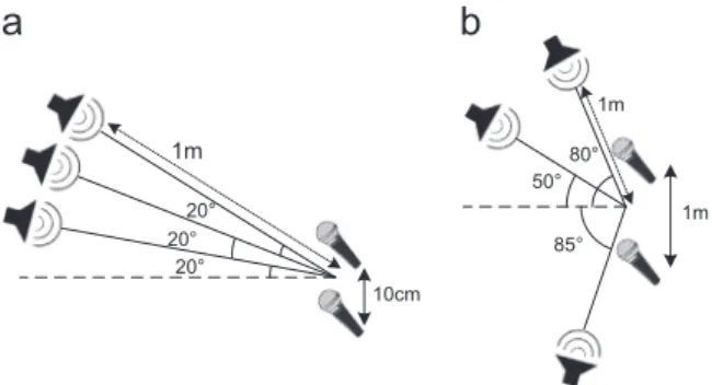
Xft¼ XK k¼1 WfkHkteiϕkftA pk estþnft pk¼j 8kAKj; j¼1…J ð12Þ where K represents the total number of components (K¼PjKj ). For later use, we define the vectorsYftsuch thatYft¼PKk¼1WfkHkteiϕkftApestk. The idea behind this fra-mework is that the same model components be assumed for both channels. The estimated channel coefficients account for the phase and attenuation difference between channels for individual sources.nftis the vector represent-ing the reconstruction error on two channels and is 1m 20° 20° 20° 10cm 1m 1m 80° 50° 85°

Fig. 1. Source-mic configuration of (a) scenarios 1, 3 and 4, and (b) scenario 2.

Table 1

Experimental parameter setting. Number ofRgsegments 50 Number ofΘsegments 180 Nonlinearity parameterα 20 Signal duration 10 s Sampling rate 16 kHz STFT frame size 1024 STFT frame shift 512 Number of iterations 500

(5)

presumed with zero-mean Gaussian distribution for both channels independent from each other. Hence, the like-lihood of the parameters Z¼W;H;

Φ

is obtained as below: pðXftj Þ ¼Z ∏ i;f;t 1

πσ

2exp XiftYift

σ

2 ð13Þ

An iterative algorithm for maximizing the likelihood function is now developed. The derivation steps can be found inAppendix A. The update relations are obtained as follows: Wfk¼ P i;t Hkt

β

kft Re Xn_ikfteiϕkft_Apk est;i h i P i;t H2kt A pk est;i 2

β

kft ; Wfk’ Wfk P fWfk ð14Þ Hkt¼ P i;f Wfk

β

kft Re XnikfteiϕkftA pk est;i h i P i;f W2fkA pk est;i 2

β

kft ð15Þ sin

ϕ

kft ¼ Q1kft ffiffiffiffiffiffiffiffiffiffiffiffiffiffiffiffiffiffiffiffiffiffiffiffiffi Q21kftþQ 2 2kft q cos

ϕ

kft ¼ Q2kft ffiffiffiffiffiffiffiffiffiffiffiffiffiffiffiffiffiffiffiffiffiffiffiffiffi Q2 1kftþQ22kft q ð16Þ

where the parameters

β

kft,Xikft,Q1kftandQ2kftare defined inAppendix A.

The

β

kftparameter is set to

β

kft¼WfkHkt=PkWfkHkt at each iteration.

To avoid scaling ambiguity, the columns of W are normalized. The iterative algorithm steps are executed in the following order:

(1) The initial values of the set of parametersZare set to those obtained via factorizing the primary source estimatesZbm.

(2) Xis updated according to(A.5)in the appendix. (3) The parametersZ¼W;H;

Φ

are updated according

to Eqs.(14)–(16). −100 −50 0 50 100 0 0.5 1 0 50 100 150 200 250 θ R g

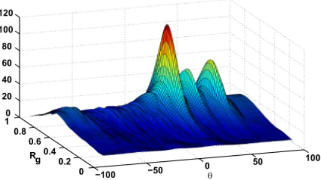
Fig. 2.2-D spectrum for anechoic mixture of scenario 1.

−100 −50 0 50 100 0 0.5 1 0 20 40 60 80 100 120 140 θ R g

Fig. 3.2-D spectrum for anechoic mixture of scenario 2.

−100 −50 0 50 100 0 0.2 0.4 0.6 0.8 1 0 50 100 150 200 250 θ R g

Fig. 4.2-D spectrum for reverberant mixture of scenario 4.

−100 −50 0 50 100 0 0.5 1 0 100 200 300 θ R g

Fig. 5.2-D spectrum for anechoic mixture of scenario 1 obtained without applying non-linearity.

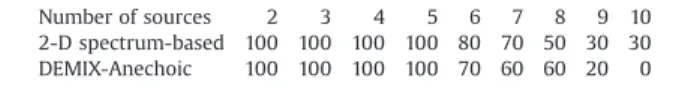
Table 2

Percentage of correct estimation of the number of sources. Number of sources 2 3 4 5 6 7 8 9 10 2-D spectrum-based 100 100 100 100 80 70 50 30 30 DEMIX-Anechoic 100 100 100 100 70 60 60 20 0

(6)

(4)

β

is updated.

The complex spectrogram of the individual sources is ultimately reconstructed according to the following expression:

Sjft¼

X

kAKj

WfkHkteiϕkft ð17Þ

The time-domain source signals can easily be derived by applying inverse STFT operation to(17).

4. Experiments

The mixture signal is synthetically generated using the Roomsim Toolbox[7]for a rectangular room of dimensions 6.253.752.5 m and omnidirectional microphones. The source and microphone height are set to 1.1 m. The position of the microphone centers in (x,y) coordinates lies at (1.56 m, 1.87 m). We evaluate our proposed method under 4 different experimental settings. In the first and second scenarios, we consider anechoic environments. The respective positions of the microphones and sources in the room for scenarios 1, 3 and 4 are the same and shown in Fig. 1a. A different arrangement is considered in scenario 2 (Fig.1b) accounting for the cases where the source signal may encounter a different attenuation in each channel. For scenarios 3 and 4, a moderate reverberation condition is simulated and the impulse responses are derived by assuming the reverberation times of T60¼50 ms and

T60¼100 ms respectively using Campbell et al. [7]. The relation between room reverberation time and absorption coefficient of the surfaces given in Gustafsson et al.[12]is utilized for generating the impulse responses correspond-ing to each case.

The male and female speech signals are taken from dev2 dataset of the SiSEC'08 “underdetermined speech and music mixtures” task [28]. The common parameter setting for all scenarios is listed inTable 1.

4.1. Evaluating source counting and channel estimation

The 2-D spectra for a single synthetic mixture of 3 male speech sources are represented inFigs. 2–4, corresponding to scenarios 1, 2 and 4 respectively. The inferred peak locations for anechoic scenarios 1 and 2 are obtained as

Rg1¼ ½0:72;0:72;0:72,

θ

g1¼ ½201;401;591 andRg2¼ ½0:56; 0:8;0:82,

θ

g2¼ ½831;471;791 which shows a near per-fect matching with the actual simulated impulse responses of the channel and source directions. The trueRgvalues for anechoic mixtures of scenarios 1 and 2 are [0.719 0.729 0.737] and [0.553 0.819 0.833] respectively. The need for considering a dimension corresponding to the amplitude response (Rg) in the spectrum is revealed when we deal

with cases similar to scenario 2 where the microphone spacing is larger and leads to different attenuation of the source signals received at each microphone.

Adding reverberation reduces the sparsity in the TF representation hence the peaks for scenario 4 are less sharp but they are still easily detectable by our peak finding algorithm. The corresponding channel parameters are obtained asRg4¼ ½0:68;0:72;0:72,

θ

g4¼ ½211;401;591. To measure the effectiveness of the nonlinear function applied in Eq. (8), we evaluate the 2-D spectrum for anechoic mixture of scenario 1 without applying the non-linearity. As can be seen inFig. 5, the peaks are wider w.r.t. the 2-D spectrum inFig. 2. Obviously, sharper peaks emerge in the spectrum when non-linearity is applied.

In order to evaluate our proposed source counting method, the rate of success of the algorithm in the estimation of the true number of sources is calculated and reported inTable 2. For this purpose,Jsources are synthetically mixed together. This is done forJfrom 2 to 10. Taking the first channel as the reference, the mixing coefficient of the second channel corre-sponding to sourcejcan be written as

a2j¼

κ

jexp i2

π

f

δ

j

fs

ð18Þ wherefsis the sampling frequency,

κ

j represents the relative mixing gain and

δ

jdenotes the relative time delay in samples. The mixing parameters are generated assuming dm¼1 cm with different relative positions of the sources and micro-phones and are listed inTable 3. For eachJ, we generate 10 different mixtures by randomly selecting the original signals from speech/music sources of the dev2 dataset. The mixing parameters are obtained assuming an arrangement similar to scenario 2 with the difference that the source directions are assumed to be uniformly spaced in the interval ½0

π

. The results are compared with the results of the DEMIX-Anechoic method[3]which are obtained using the software provided in Arberet[2]. Like in their work, the success rate is calculated as the percentage of correct estimations out of 10 trials. As can be observed, the algorithms perform perfectly up to 5 sources and the performance of our source counting algorithm is quite comparable and sometimes better than the DEMIX-Anechoic algorithm.

To also evaluate the mixing parameter estimation performance, the mean mixing parameter error (MMPE) is calculated similar to the mean direction error (MDE) proposed in Arberet et al. [3]. Given the true mixing parameter values

κ

¼ ½

_κ

1…

κ

J;

δ

¼ ½

δ

1…

δ

J and the esti-mated ones

κ

^¼ ½

κ

^1…

κ

^J;

δ

^¼ ½

δ

^1…

δ

^Jthe MMPE is defined for both of the amplitude and delay parameters as below: MMPE

κ

;

κ

^¼min PASJ 1 J XJ j¼1

κ

j

κ

^PðjÞ Table 3

Mixing parameters used to simulate mixtures with up to 10 sources.

Parameter S1 S2 S3 S4 S5 S6 S7 S8 S9 S10

κj 0.62 1.09 0.87 1.74 1.35 1.23 0.95 1.53 0.72 0.54

(7)

MMPE

δ

;

δ

^ ¼min PASJ 1 J XJ j¼1

δ

j

δ

^PðjÞ ð19Þ

where SJis the permutation group of sizeJ. Toward this goal, theJhighest peaks of the 2-D spectrum found by the

peak finder algorithm are considered as the estimated mixing coefficient values of the sources. Similarly, for DEMIX-Anechoic algorithm, we set and fix the number of sources to J. To measure the error in terms of relative precision, the relative mean mixing parameter errors

2

4

6

8

10

−2

10

−1

10

0

Numbr of sources

Relative mixing amplitude error

2−D Spectrum−based method DEMIX−Anechoic method

2

4

6

8

10

−3

10

−2

10

−1

10

0

Numbr of sources

Relative mixing delay error

2−D Spectrum−based method DEMIX−Anechoic method

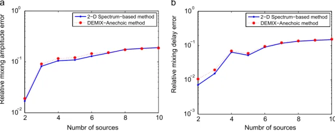
Fig. 6.Relative mean mixing parameter error (RMMPE) as a function of the number of sources: (a) Relative mixing amplitude error, (b) Relative mixing delay error. 5 10 15 20 25 30 −0.12 −0.1 −0.08 −0.06 −0.04 −0.02 0 order log−likelihood 5 10 15 20 25 30 −0.8 −0.6 −0.4 −0.2 0 order log−likelihood

Fig. 7. Log-likelihood function against order for (a) male and (b) female sources.

Table 4

BSS Evaluation metrics obtained for scenario 1.

Method SDR (dB) SIR (dB) SAR (dB)

Complex NMF 12.8 18 14.3

Binary masking 8.9 17.7 10.1 l0-norm minimization 6.1 10.7 9.5

Table 5

Complex NMF 11.7 16.6 13.2

Binary masking 9 15.1 9.6

l0-norm minimization 5.2 8.4 9.5

Table 6

Complex NMF 9.7 11.6 13.8

Binary masking 7.5 12.2 9.3

l0-norm minimization 7.7 10 10.2

Table 7

Binary masking 4.7 8.8 8.5

(8)

(RMMPE) are defined as RMMPE

κ

;

κ

^¼ MDE

κ

;

κ

^ min jaj0

κ

j

κ

j 0 RMMPE

δ

;

δ

^ ¼MDE

δ

; ^

δ

min jaj0

δ

j

δ

j 0 ð20Þ

where the denominators denote the minimum distance between the true mixing parameter values. RMMPE values for amplitude and delay parameters are plotted inFig. 6a and b respectively against the number of the sources. Because of the higher resolution needed for these experi-ments, we have used 18,000

θ

segments and 100 Rg segments for evaluating the 2-D spectrum to achieve an angular resolution of 0.011and normalized amplitude resolution of 0.01. It can be seen that our proposed algorithm outperforms DEMIX-Anechoic method up to 6 sources in terms of delay parameter relative error and up to 7 sources in terms of amplitude parameter relative error. Adding more sources, the two algorithms show nearly the same performance.

4.2. Model order selection

To get an insight of the proper number of components needed for modeling each source, a model order selection scheme is implemented here. This method is applied to the primary source spectrograms given by binary masking. The initial values of the elements of Wbm _and _Hbm _are drawn randomly from the absolute value of a standard Gaussian distribution plus 1 (absðNð0;1ÞÞþ1). The Wbm elements are normalized according to14. Initial values of

Φ

bm

are drawn from a uniform distribution over the interval ½

_{π π}

. The update algorithm is iterated 500 times. The log-likelihood function is evaluated against a range of order valueskAf3…30g. The likelihood graphs for the mixture of 3 male and 3 female speech signals generated under scenario 1 are represented in Fig. 7a and b respectively. We exploit the BIC metric defined as

BIC¼ 2LLþNplogðNobsÞ ð21Þ

where LL represents the corresponding log-likelihood vector,Npdenotes the number of model parameters and

Nobsis the number of observed samples associated with

each value in LL. The order value corresponding to the minimum obtained BIC metric is taken as the optimal number of model components. This leads to order values of [5 6 6] and [7 8 7] for the male and female sources, respectively. For mitigating the computational burden, we do not re-execute the model order selection algorithm for each mixture in the next step. Instead, we take a fixed number of components considered for each source in our model based on the above experimentsðKj ¼8; j¼1…JÞ.

4.3. Source separation evaluation

Here, we are to evaluate the performance of our proposed source separation algorithm using the extended multichannel model. We generated 10 mixtures of 3 (male and/or female) speech signals using the impulse responses obtained through Campbell et al. [7]. The separation quality is measured by calculating the evaluation metrics including Signal to Distortion Ratio (SDR), Signal to Inter-ference Ratio (SIR) and Signal to Artifact Ratio (SAR)[29].

−100 −50 0 50 100 0 0.2 0.4 0.6 0.8 10 20 40 60 80 100 120 θ Rg

Fig. 8. 2-D spectrum for reverberant mixture withT60¼500 ms.

0 5 10 15 20 25 30 0.45 0.5 0.55 0.6 0.65 0.7 0.75 0.8 0.85 0.9 Attenuation (dB)

Relative Peak height

Fig. 9.Relative peak height against the source signal attenuation for reverberant mixture withT60¼500 ms.

0 100 200 300 400 500 −5 0 5 10 T₆₀(ms) Average SDR(dB) Complex NMF Binary masking l 0−norm minimization

(9)

The performance measures averaged over all sources and all mixtures are reported inTables 4–7corresponding to 4 scenarios. As comparison materials, the results of binary masking and l0-norm minimization algorithms are also

evaluated using the reference software in Vincent et al. [28]and are listed in the tables. It can be observed that our proposed method outperforms both of the state-of-the-art methods in all evaluation metrics. The algorithm works also in moderate reverberant environments since the sparsity in the TF domain is still sufficient for pure peaks to emerge in the 2-D spectrum.

5. Discussion

We now investigate to what extent the algorithm performance is still acceptable when we are to handle longer than the intended reverberation times. Toward this objective, the effectiveness is first measured in the first stage, i.e. the channel estimation and source counting, and then source separation performance is assessed against differentT60values.

Fig. 8represents the 2-D spectrum for the arrangement ofFig. 1a withT60¼500 ms. The proposed spectrum-based approach is apparently still applicable in highly reverber-ant environments for the purpose of source counting and angle of arrival estimation. The corresponding channel parameters are obtained as Rg¼ ½0:7;0:7;0:66;

θ

g¼ ½201; 401;591in this case. As can be observed, the peaks of the spectrum are getting wider by increasing the reverbera-tion time but the number of the sources and source directions are obtained with the same accuracy as the moderately reverberant case according to our experimen-tation. To also investigate the effectiveness of the relative amplitude threshold (0.5) in this highly reverberated case, we reduce the strength of one source in the mixture of 3 sources and plot the relative peak height corresponding to that source as a function of the source strength (the attenuation applied to the signal). The result is shown in Fig. 9. It can be observed that the chosen fixed threshold value (0.5) is quite effective in detecting the peak up to 12 dB reduction in the source signal amplitude. From this analysis, we can state that the parameter choice will be related to the signal conditions (reverberation and SNR) in a practical deployment.

The performance of the source separation is shown in Fig. 10in terms of average SDR. The average performance metrics are calculated by taking the average over all sources and all mixtures in the dev2 database (speech/ music). The performance degrades when increasing the reverberation time for all of the methods. This is an expected result since there is no model for multipath propagation, but complex NMF still outperforms the other methods. Nevertheless, the satisfying results of the first stage can be exploited in a suitable framework for source separation in highly reverberant conditions. Taking rever-beration into account, most of the source separation methods work based on the spatial covariance matrix modeling [4,9] and use the Expectation Maximization (EM) algorithm for maximizing the data likelihood. The EM algorithm is very sensitive to initialization. The mixing coefficients obtained in the first step could provide proper initialization for these approaches. For this purpose, we propose to use the estimated channel parameters given in (10). We have obtained the average performance metrics for the full-rank method of Duong et al.[9]. The metrics are evaluated for two different reverberation conditions (T60¼150 ms andT60¼500 ms) represented in Tables 8 and9 respectively. We also compare our proposed initi-alization scheme with the hierarchical clustering-based initialization scheme proposed in[9]. We execute 50 EM algorithm iterations and the number of clusters for hier-archical clustering is set to 30. As it can be observed, in low reverberation condition (T60¼150 ms), our proposed method outperforms that of Duong et al. [9]with both initialization schemes. It is also evident that our proposed initialization makes the EM algorithm to lead to better results. In higher reverberation, the full-rank method is performing better than the complex NMF approach and again better performance is achieved using our proposed initialization scheme.

6. Conclusion

In the first step, we developed a novel scheme for source counting and channel estimation in anechoic or moderate reverberant environments introducing a 2-D spectrum over both phase and attenuation difference between the channels.

Table 8

Average performance metrics obtained forT60¼150 ms.

Full-rank method with our proposed initialization scheme 6.9 10.8 10.5 Full-rank method with hierarchical clustering-based initialization 6.2 10.0 9.4

Table 9

Average performance metrics obtained forT60¼500 ms.

Full-rank method with our proposed initialization scheme 4.2 5.3 8.9 Full-rank method with hierarchical clustering-based initialization 3.61 4.9 8.1

(10)

Secondly, an extension of the complex factorization framework was developed for the purpose of source separation which uses the channel mixing coefficients estimated in previous step. The initial values of the factors are set to those obtained from primary source spectrogram estimates given by binary masking. The average BSS performance metrics shows the superiority of our algo-rithm over all three evaluation criteria for all different considered source separation scenarios.

We have also introduced a model order selection scheme using the BIC metric for inferring the required number of components for modeling each source. This algorithm can be applied to the primary source spectro-gram estimates.

Assuming a prior distribution for theHparameters can be helpful if we set up a training procedure for obtaining the optimal values of the hyperparameters of the prior distribution and can be considered in future work for the purpose of performance improvement.

Acknowledgments

This research was funded by the KU Leuven research Grant GOA/14/005 (CAMETRON).

Appendix A. Derivation of the update relations for the extended multichannel model

We are to solve the following optimization problem: minimize Z fðZÞ ¼ X i;f;t XiftYift 2 subject to X f Wfk¼1ðk¼1…KÞ ðA:1Þ We define the following auxiliary function with aux-iliary parametersZ¼ fXginspired from Kameoka et al.[15]

fþZ;Z¼X i;k;f;t XikftWfkHktejϕkftA pk est;i 2

β

kft ðA:2Þ where

β

kftcan be any positive number satisfyingPk

β

kft¼1. The auxiliary functionfþðZ;ZÞshould satisfy

fðZÞ ¼min Z

fþðZ;ZÞ ðA:3Þ If the above condition is satisfied, it can be shown based on Lee and Seung [16] that fðZÞ is non-increasing under the updatesZ_’argmin Z f þ ðZ_;ZÞandZ_’argminZf þ ðZ_;ZÞ.

fþðZ;ZÞis an auxiliary function forfðZÞif

X k Xikft¼Xift ðA:4Þ fþðZ;ZÞis minimized w.r.t.Zwhen Xikft¼WfkHktejϕkftA pk

est;iþ

β

kftðXiftYiftÞ ðA:5Þ Eq.(A.5)can be derived by adding the Lagrange multi-plier term to the auxiliary function of Eq.(A.2):

Λ

ðX;

λ

Þ ¼fþðZ;ZÞþ

λ

ift X k XikftXift ! ðA:6Þ

and then taking the derivative of (A.6) w.r.t. Xikft and setting it to zero, we have

2Xikft2WfkHktejϕkftAestpk;i¼

λ

ift

β

kft ðA:7Þ

λ

ift is obtained by summation overkon both sides of (A.7)and applying the constraint(A.4):

λ

ift¼2ðXiftYiftÞ ðA:8Þ Consequently,Xikft is obtained as given by(A.5). Sub-stituting(A.5)in the expression (A.2), we determine the minimum value of the auxiliary function which is equal to

fðZÞ, so condition(A.3)is satisfied.

DifferentiatingfþðZ;ZÞ w.r.t.Wfk and Hkt and setting them to zero, leads to the update relations for these parameters as stated in(14) and (15).

Deriving the update relations for

ϕ

kftis not as straight-forward as the above parameters. The first derivative of the auxiliary functionfþðZ;ZÞw.r.t.

ϕ

kftis proportional to the following expression:

∂fþðZ_;ZÞ ∂

ϕ

kft p X i WfkHktReðA pk est;iX n ikftÞ n o sin

ϕ

kft þ WfkHktImðA pk est;iX n ikftÞ n o cosð

_ϕ

kftÞ ðA:9Þ

Since we assumed the first channel as reference, the channel coefficient on the first channel,Apk

est;1¼1 in accor-dance with(10). Thus, setting(A.9)to zero, we obtain the following update relation for

ϕ

kftcoefficients:

Q1kft¼Im X1kft Im Apk est;2X n 2kft Q2kft¼Re X1kft þRe Apk est;2X n 2kft

ϕ

kft¼atan Q1kft Q2kft ðA:10Þ Actually, the above solution does not result in a unique value for

ϕ

kft. The unique solution is achieved by noticing the point that the second derivative of the cost function

fþðZ;ZÞw.r.t.

ϕ

kftshould be positive: ∂2_fþ_ð_Z_;_Z_Þ ∂

ϕ

2 kft psin

ϕ

kft ImX1kft Im Apk est;2X n 2kft n o þcosð

_ϕ

kftÞ fReðX1kftÞþReðApestk;2X n 2kftÞgZ0 ðA:11Þ Satisfying the above condition will specify the unique solution inferred from(A.10). It can be implied from(A.11) that the sine and cosine of

ϕ

kftshould have the same signs as the nominator and denominator of (A.10)respectively. The form of the update relation stated in(16)will satisfy this. References

[1] S. Araki, H. Sawada, R. Mukai, S. Makino, A novel blind source separation method with observation vector clustering, in: Proceed-ings of IWAENC, 2005, pp. 117–120.

[2] S. Arberet, Demix-anechoic Software Reference Website. URL

〈https://sites.google.com/site/simonarberet/codes/〉.

[3]S. Arberet, R. Gribonval, F. Bimbot, A robust method to count and locate audio sources in a multichannel underdetermined mixture, IEEE Trans. Signal Process. 58 (1) (2010) 121–133.

[4] S. Arberet, A. Ozerov, N.Q. Duong, E. Vincent, R. Gribonval, F. Bimbot, P. Vandergheynst, Nonnegative matrix factorization and spatial covariance model for under-determined reverberant audio source separation, in: 2010 10th International Conference on Information

(11)

Sciences Signal Processing and their Applications (ISSPA), IEEE, Kuala Lumpur, Malaysia, 2010, pp. 1–4.

[5] N. Bertin, R. Badeau, E. Vincent, Fast Bayesian nmf algorithms enforcing harmonicity and temporal continuity in polyphonic music transcription, in: WASPAA, 2009, pp. 29–32.

[6]P. Bofill, M. Zibulevsky, Underdetermined blind source separation using sparse representations, Signal Process. 81 (11) (2001) 2353–2362.

[7]D. Campbell, K. Palomaki, G. Brown, A matlab simulation of“ shoe-box”room acoustics for use in research and teaching, Comput. Inf. Syst. 9 (3) (2005) 48.

[8] O. Dikmen, A.T. Cemgil, Unsupervised single-channel source separa-tion using bayesian nmf, in: IEEE Workshop on Applicasepara-tions of Signal Processing to Audio and Acoustics, 2009. WASPAA'09. IEEE, New Paltz, New York, USA, 2009, pp. 93–96.

[9]N.Q. Duong, E. Vincent, R. Gribonval, Under-determined reverberant audio source separation using a full-rank spatial covariance model, IEEE Trans. Audio Speech Lang. Process. 18 (7) (2010) 1830–1840. [10]C. Févotte, A. Ozerov, Notes on nonnegative tensor factorization of

the spectrogram for audio source separation: statistical insights and towards self-clustering of the spatial cues, Explor. Music Contents (2011) 102–115.

[11] D. FitzGerald, M. Cranitch, E. Coyle, Non-negative tensor factorisa-tion for sound source separafactorisa-tion, in: Proceedings of the Irish Signals and Systems Conference, Dublin Institute of Technology, Dublin, Ireland, 2005.

[12]T. Gustafsson, B.D. Rao, M. Trivedi, Source localization in reverberant environments: modeling and statistical analysis, IEEE Trans. Speech Audio Process. 11 (6) (2003) 791–803.

[13] M.Z. Ikram, D.R. Morgan, A beamforming approach to permutation alignment for multichannel frequency-domain blind speech separa-tion, in: 2002 IEEE International Conference on Acoustics, Speech, and Signal Processing (ICASSP), vol. 1, IEEE, Orlando, Florida, 2002, pp. I–881.

[14] R. Jaiswal, D. FitzGerald, D. Barry, E. Coyle, S. Rickard, Clustering nmf basis functions using shifted nmf for monaural sound source separation, in: 2011 IEEE International Conference on Acoustics, Speech and Signal Processing (ICASSP), 2011, pp. 245–248. [15] H. Kameoka, N. Ono, K. Kashino, S. Sagayama, Complex nmf: a new

sparse representation for acoustic signals, in: IEEE International Conference on Acoustics, Speech and Signal Processing, 2009. ICASSP 2009. IEEE, Taipei, Taiwan, 2009, pp. 3437–3440. [16] D.D. Lee, H.S. Seung, Algorithms for non-negative matrix

factoriza-tion, in: Advances in Neural Information Processing Systems, 2001, pp. 556–562.

[17] B. Loesch, B. Yang, Blind source separation based on time–frequency sparseness in the presence of spatial aliasing, in: Latent Variable Analysis and Signal Separation, Springer, St. Malo, France, 2010, pp. 1–8.

[18] Y. Mitsufuji, A. Roebel, Sound source separation based on non-negative tensor factorization incorporating spatial cue as prior, New

Paltz, New York, USA, knowledge, in: 2013 IEEE International Conference on Acoustics, Speech and Signal Processing (ICASSP), 2013, pp. 71–75.

[19] F. Nesta, M. Omologo, P. Svaizer, Multiple tdoa estimation by using a state coherence transform for solving the permutation problem in frequency-domain bss, in: IEEE Workshop on Machine Learning for Signal Processing, 2008. MLSP 2008. IEEE, Cancun, Mexico, 2008, pp. 43–48.

[20]A. Ozerov, C. Fevotte, Multichannel nonnegative matrix factorization in convolutive mixtures for audio source separation, IEEE Trans. Audio Speech Lang. Process. 18 (3) (2010) 550–563.

[21]V.G. Reju, S.N. Koh, I.Y. Soon, Underdetermined convolutive blind source separation via time–frequency masking, IEEE Trans. Audio Speech Lang. Process. 18 (1) (2010) 101–116.

[22]R. Saab, O. Yilmaz, M.J. McKeown, R. Abugharbieh, Underdetermined anechoic blind source separation via lq-basis-pursuit, IEEE Trans. Signal Process. 55 (8) (2007) 4004–4017.

[23]H. Sawada, S. Araki, R. Mukai, S. Makino, Grouping separated frequency components by estimating propagation model para-meters in frequency-domain blind source separation, IEEE Trans. Audio Speech Lang. Process. 15 (5) (2007) 1592–1604.

[24]H. Sawada, H. Kameoka, S. Araki, N. Ueda, Multichannel extensions of non-negative matrix factorization with complex-valued data, IEEE Trans. Audio Speech Lang. Process. 21 (5) (2013) 971–982. [25]H. Sawada, R. Mukai, S. Araki, S. Makino, A robust and precise

method for solving the permutation problem of frequency-domain blind source separation, IEEE Trans. Speech Audio Process. 12 (5) (2004) 530–538.

[26] P. Smaragdis, J. Brown, Non-negative matrix factorization for poly-phonic music transcription, in: 2003 IEEE Workshop on Applications of Signal Processing to Audio and Acoustics, 2003, pp. 177–180. [27] E. Vincent, Complex nonconvex l p norm minimization for

under-determined source separation, in: Independent Component Analysis and Signal Separation, Springer, London, UK, 2007, pp. 430–437. [28] E. Vincent, S. Araki, P. Bofill, The 2008 signal separation evaluation

campaign: a community-based approach to large-scale evaluation, in: Independent Component Analysis and Signal Separation, Springer, Paraty, Brazil, 2009, pp. 734–741.

[29]E. Vincent, R. Gribonval, C. Févotte, Performance measurement in blind audio source separation, IEEE Trans. Audio Speech Lang. Process. 14 (4) (2006) 1462–1469.

[30]T. Virtanen, Monaural sound source separation by nonnegative matrix factorization with temporal continuity and sparseness cri-teria, IEEE Trans. Audio Speech Lang. Process. 15 (3) (2007) 1066–1074.

[31]S. Winter, W. Kellermann, H. Sawada, S. Makino, Map-based under-determined blind source separation of convolutive mixtures by hierarchical clustering and l1-norm minimization, EURASIP J. Appl. Signal Process. 2007 (1) (2007) 81.

[32]O. Yilmaz, S. Rickard, Blind separation of speech mixtures via time– frequency masking, IEEE Trans. Signal Process. 52 (7) (2004) 1830–1847.