Modelling a Smart Motorway
Edward Richardson1, Philip Davies2, David Newell31 Capgemini, Woking, UK [email protected] 2 Bournemouth University, Bournemouth, UK
[email protected] 3Bournemouth University, Bournemouth, UK
Abstract— The increasing number of vehicles in the UK is putting high levels of strain upon the motorway’s infrastructure. Smart Motorways have been implemented in the UK using smart technology to try and reduce congestion. To test systems before they are physically built they are simulated using objects models and GIS data. This paper has modelled a new smart traffic light system for a slip road joining a smart motorway. The smart traffic light models have been simulated alongside Driver Behavior models. The driver behavior models have been designed to validate that the smart traffic light system can adapt to continuously fluctuating traffic flow. The smart traffic light system has been successfully validated and reduced the number of congestion alerts by 80% on the smart motorway.
1.INTRODUCTION
In the UK traffic congestion is putting increasing strain upon the motorway infrastructure. The increasing number of cars has resulted in heavy congestion and motorways reaching capacity. Smart technology was concluded the best option with the smallest impact on the public and the environment [7]. Smart technology is being used in several different applications to keep the traffic flowing. One of the applications is to have Smart Traffic Lights (STL) that can communicate with the motorway sensors to aid traffic flow from joining slip roads.
Smart Motorways (SM) could improve traffic flow and help to manage traffic especially when unpredictable events such as accidents occur. A simulator will provide an insight into how smart technology impacts upon traffic flow. It will aid in fine tuning the smart technology, especially simulating traffic flow controlled by STL to validate the impact upon traffic flow.
2.LITERATURE REVIEW
There is currently a growing trend for traffic simulators to use Geography Information System (GIS) data combined with simulator programmes. GIS data is used to create accurate base maps for the simulator including varying topography. GIS shape files are used to simulate the dynamics of an object such as a vehicle or a
pedestrian. The simulation of the objects requires models to determine the possible actions of the object.
Research carried out by Miller et al [14] has highlighted the variety of models required for an accurate traffic simulator. There are two main types of model required, a traffic model and a driver behavior model. Previous papers ([4],[12],[19]) have suggested the models required in a simulator. However, they are not designed for SM.
2.2 Vehicle Models
Zhao et al [21] created a simulator to predict marine incidents and focused on predicting ship collisions. The simulation of ship traffic flow has the same issues as motorway traffic flow due to the variety in vehicle sizes and speeds. Their approach was to create shape files in GIS that could be used in a simulator with the exact shape of different ships. This would allow the simulator to be able to predict more accurately the interaction between vessels of different sizes rather than having different vessels as generic object shapes.
Liao and Yen [11] and Sasso and Biles [15] simulated vehicles as simple objects in 2D. Their approaches focused more on the overall flow of traffic. However, the main drawback is it presumes all objects act in the same way which is not the case for vehicles with different drivers. Zhao et al [21] have the problem of having two separate databases however they specify the shape of the vessels and are not treating them all as the same generic object. The main issue is the lack of behavioural models in the simulators and maintaining separate databases.
2.3 Macroscopic or Microscopic View Point
The modelling of a simulator is controlled by the level of the simulator view and the objects being simulated. A simulator can be either macroscopic, mesoscopic or microscopic. The level of the simulator view is most commonly macroscopic with multiple papers ([1],[8],[11],[20]]) focusing on this view point. However, the lack of detail is an issue especially in a complex heterogeneous system such as simulating built up urban areas. Zhao et al [21] used a macro-traffic flow approach. It could not show the individual behaviours of ships and only simulated the action of ships leaving/entering ports. Sasso and Biles [15] had a similar issue as Zhao et al [5] because they were simulating a large geographical area (Panama Cannal) where only a macroscopic view would be able to simulate it. This resulted in the ships being simulated as small rectangles and their individual behaviour not being simulated.
Huang and Pan [8] built a simulator for the prediction of the best route for emergency responders to an incident. They used a macroscopic view point which provided a good overall summary but does not allow for how the behaviour of drivers at specific junctions could impact upon the emergency responders route. Liao and Yen [11] simulated a comparable emergency event as Huang and Pan [8] for an earthquake evacuation. Both simulator events share similar issues in terms of sudden heavy traffic flow. Liao and Yen [11] used a micro-traffic flow simulator. The strength of this approach over macro is it can focus on specific road junctions clearly showing the potential issues. It does not show the overall traffic flow which may be heavily impacted by a road junction that is out of the scope of the micro simulator.
Khalesian and Delavar [9] simulated a highway where it could have been viewed from a macroscopic view point similar to that of Huang and Pan [8] but they decided to use a microscopic view point. Khalesian and Delavar [9] simulated the driver’s
behaviour which on a motorway is an important factor to consider with multiple lanes. A microscopic simulator especially for a motorway could be extrapolated for a larger network and applied to multiple settings.
2.4 Behaviour Models
Khalesian and Delavar [9] designed several models that each object follows rather than the overall model being applied to all objects. The approach of Khalesian and Delvar [9] is one that can be applied to any simulator. It is more realistic as each vehicle has an individual behavior model which allows for the vehicles to interact. Dallmeyer et al [4] modelled the cars following the non-cell approach. This approach allows for an object orientated simulator that is more realistic as objects can independently act. Dallmeyer et al [4] additionally modelled a prediction method for the direction of the traffic in an urban setting. Dallmeyer et al [4] did not include in their behaviour models the different vehicles in an urban environment and how they will behave differently.
3 RESEARCH QUESTIONS
The models required to determine how the objects interact is a crucial part of any simulator and is a gap we have identified in this literature review. There is currently a lack of traffic and behaviour models for simulators using GIS data. There were no papers regarding simulating SM identified during this literature review. In consideration of these factors we have proposed several new traffic and behaviour models. The following hypotheses have been developed to validate if the SM improved the traffic flow.
3.1 Hypotheses
1. The STL will reduce the number of congestion alerts in comparison to a
free-flowing slip road.
2. The STL will reduce the number of congestion alerts in the left lane in comparison to a free-flowing slip road.
3. The STL will reduce the number of congestion alerts in the middle lane in comparison to a free-flowing slip road
4 METHOD
There are two types of model that will be proposed in this paper; traffic and behavioural. The first step will be to define each term for the different models. This will be carried out by investigating previous definitions used by papers that have suggested simulator models.
The models that are proposed will be either new models that are specific to a SM or will be adapted from previous models. The models will be including the most relevant elements from previous models that have been identified from literature reviews ([13], [18]). The adapted models will be selected from literature reviews that have validated in traffic simulators. Due to the variety of features on a SM, the models will be focused on a STL system and how the driver behaviour will impact upon the technology.
The models will be built in Simulink using the model elements. Random number Generators (RNG) will be used to create realistic vehicle parameters with a set mean and variance. The number of vehicles joining from the slip road and on the motorway will be based upon peak traffic flow numbers on the M3 [7].
The simulation will be at a microscopic level as the models are object orientated and the simulator is designed to see how the STL adapts. To simulate vehicles with different properties an RNG that has a fixed mean and variance will be used for determining each model parameter. The mean and variance are based upon real data to be as realistic as possible. The STL can be refined to allow more vehicles through depending on the impact on the motorway traffic flow.
5 SMART MOTORWAY
A SM is defined as a motorway that uses smart technology to monitor and control traffic flow. SM vary in design to be adapted to the setting of the motorway especially in locations where several motorways merge.
The SM is monitored by a system called Motorway Incident Detection and Automatic Signaling (MIDAS) that can differentiate between congestion and queued traffic [10]. The MIDAS system controls the variable speed limits (VSL) shown on the gantries above a motorway and are designed to help with the traffic flow by reducing the stop/start traffic conditions from occurring.
6 TRAFFIC MODELS
The term ‘Traffic Model’ is used in a variety of different contexts and therefore has multiple definitions. Song et al. [16] define a traffic model as a model that influences how objects behave, interact with each other and their environment. Boxill and Lu [2] defined a traffic model as a model that defines the environment that an object interacts with. Taplin [17] defined a traffic model as modelling the flow of traffic based on dynamic models. The term Traffic Model is defined in this paper as a model that defines the environment of the simulator. This includes models such as the STL and SM models.
We developed a model focusing on the application of a STL and how it can reduce congestion on a SM by controlling the slip road traffic. We have included how driver behavior will impact upon the STL system.
6.1Ramp Metering
Ramp metering is the term used for traffic lights controlling the traffic flow joining a motorway where a STL calculates when to release the traffic [10]. To simulate a STL controlling the flow from a slip road there are several models to consider. These models require live information being provided from both the slip road and the SM.
Cai et al [3] carried out the modelling of STL for an intersection that has traffic approaching from four different directions. The Queue Tracker Model (QTM) shown in equation 1 (explained in table 1) is modelled to calculate the queue length at each traffic light. The model decides which traffic queue to release next based on the queue length to reduce congestion at the junction.
Table 1 QTM Model
Model Element Element Definition O Time Occupancy (Seconds)
T Time (Seconds)
C Vehicle Count
Li Vehicle Length (Metres)
Lloop Length of Induction Loop in Road (Metres)
The model has been adapted to provide the STL with the information regarding the number of vehicles in the queue. The proposed model can now calculate how many vehicles are queued on the slip road by measuring individual vehicle size. Equation 2 (explained in table 2) is the proposed model for calculating the number of vehicles queued on the slip road. This model will be continuously calculating the length of the vehicles in the traffic queue on the slip road. The STL requires an additional model to calculate if there are any gaps in the motorway traffic.
μ =α√ql−qt
vl (2)
Table 2 QTM Model
Model Element Element Definition µ Number of vehicles in the queue
Α Mean Velocity (M/S)
ql Queue Length starting from traffic lights (M)
qt Queue Time (S)
Vl Vehicle Length (M)
6.2The Gap Analysis Model-GAP
The role of the STL is to calculate the motorways current capacity and calculate the most efficient time to release vehicles. The STL is designed to calculate the size of the gap in the motorway traffic and consider the size of the vehicle that is on the slip road. The STL can detect if a large vehicle such as a lorry is present and wait for a gap suitable for the lorry to join however the driver still has the final decision.
The QTM is used alongside the GAP to determine how quickly the queue is moving and if there are vehicles in the queue. The STL requires information from the motorway regarding the traffic density to calculate gaps in the traffic on the SM The output from the model is the size of the gaps in the traffic based upon the traffic density (equation 3, table 3).
Ga =Li+Lloop
C × (O × Vi) (3)
Table 3 GAP Model
Model Element Element Definition
Ga Size of gap in traffic (Meters) Li Vehicle Length (Meters)
Lloop Length of Induction Loop in Road (Meters) Vi Vehicle Velocity (M/S)
C Vehicle Count
7 BEHAVIOUR MODELS
The driver behaviour models are required in the simulator to show how a STL can adapt to driver’s behaviour. The definition of a driver behaviour model is a model that calculates the possible action a driver can make based upon the traffic conditions and their ability. A vehicles performance is part of a driver’s behaviour model. The objects in a simulator will require multiple models that can predict the behaviour of an object to simulate the complex decision process of a driver. A literature review carried out by Toledo [13] has been used to identify the main driver behaviour models. This literature review was used because it focused on models for a microscopic simulator and driver models for a motorway.
7.1Car Following Model
The car following model is the non-linear model designed by Gazis et al [5]. The model is based upon the idea that the lead vehicle controls the velocity and acceleration of the following vehicle. This model will influence the driver’s decision to change lane dependent upon their sensitivity and desire to change their vehicles velocity. Gazis et al [5] model does not include the driver’s ability to maintain following the vehicle in front or the driver’s reaction time. Equation 4 shows the model and table 4 explains the model.
Table 4 Car Following Model
Model Element Element Definition
Gf Lag Distance (metres)
g0f Lag space gaps at start of lane changing (metres) vf Speeds of lag vehicle (M/S)
Dt dv/ bf
bf Deceleration of target lag vehicle (M/S) Dv Level of aggressiveness of lag vehicle Vs Speed of subject vehicle (M/S) Dl Desire to change lane
7.2 The Lane Changing Gap Model
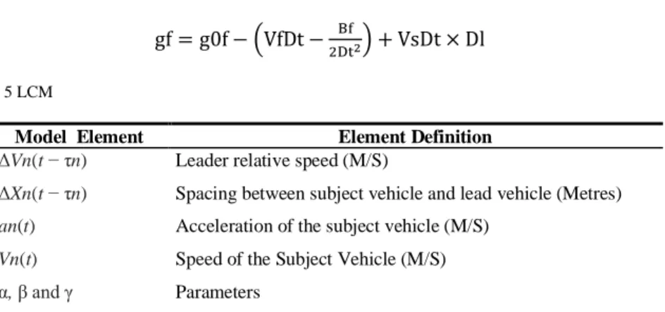
The lane changing model (LCM) will be based on the model proposed by Hidas [6], equation 5 explained in table 5. The model has been adapted to include the driver’s level of desire to change lane. The output for the model is the size of the gap for the driver to change lane. The greater the desire to change lane results in the size of gap perceived by the driver to increase in size. Another factor included in the model is the level of aggression a driver has. This presumes that a more aggressive driver is more likely to change lane than a non-aggressive driver.
gf = g0f − (VfDt − Bf
2Dt2) + VsDt × Dl (5) Table 5 LCM
Model Element Element Definition
ΔVn(t − τn) Leader relative speed (M/S)
ΔXn(t − τn) Spacing between subject vehicle and lead vehicle (Metres)
an(t) Acceleration of the subject vehicle (M/S)
Vn(t) Speed of the Subject Vehicle (M/S)
α, β and γ Parameters
In the middle lane a driver can decide to change into either the left or the right lane. Therefore, this will require an additional model where a driver can decide which lane they consider changing to. The important factors to consider here are the drivers desire to change lane, their ability to change lane and their level of desire for the lane. It is presumed that a driver in the middle lane is in this lane to overtake other vehicles and that drivers intend on being in the left lane. The decision to change lane is combined with the lane changing model as they driver may want to change lane but are not able to. Equation 6 shows the model and is explained in table 6.
Ld =Dl ×
da va
Ls (6)
Table 6 Lane Desire Model
Model Element Element Definition
Ld Desire for left or right lane-Positive value for left lane- negative value for right lane
Dl Desire to change lane Da Driver ability to change lane Va Vehicle ability to change lane
7.3 Slip Road Velocity Model
The slip road velocity model (RVM) is designed to replicate the thought process of a driver before they join the motorway. This model is required because even if the STL calculates there is a gap for the vehicles to join the motorway the driver may decide not to. Equation 7 is a model developed by Michaels and Fazio [13] that calculates the angular velocity for a vehicle joining a motorway explained in table 7. It is presumed by using this model that the slip road joining a motorway is not linear and requires the driver to join at an angle. This model does not include the length of the vehicle and presumes that all vehicles have the same rate of acceleration. The model can simulate a driver’s decision to join the motorway from the slip road which may not be determined by their vehicles ability.
W=k(Vf-Vr)/L2 (7) Table 7 RVM
Model Element Element Definition
W Angular velocity Vf Motorway vehicle speed (M/S) Vr Ramp vehicle speed (M/S) L2 Distance separation (metres) K Lateral offset (metres)
8 SIMULATION-MATLAB SIMULINK
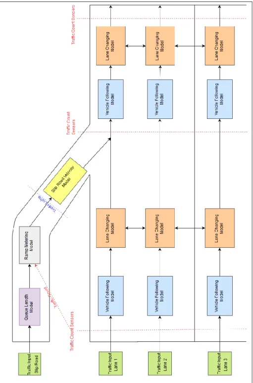
Figure 1 is a conceptual design of the SM. The slip road will be controlled by the STL that is receiving live information. The information received by the STL is before the driver behaviour models. This allows for vehicles to continuously be free flowing after the traffic readings have taken place. The sensors at the end of the motorway will measure the output of all the three lanes of traffic. The motorway will be monitored based on the traffic flow which Simulink displays in the model element ‘scope’.
In the simulator 1 unit of time is the equivalent to 10 seconds. This timescale was chosen because it allows the models to adapt in a more realistic manner and the models can be validated over a longer time. The models for the driver behaviour will be applied to a group of vehicles to validate that the output varies and not for individual vehicles. This will result in groups of vehicles changing lane rather than individuals. The total simulation time is 1.5 hours.
9 DATA ANALYSIS
The hypotheses were tested by comparing a SM and a normal motorway in the simulator. The normal motorway does not include the STL and has been replaced in the simulator by a RNG. The parameters for the RNG are based upon the overall output from the STL to be comparable. The parameters for all the driver behaviour models have been kept the same for both simulations to be comparable.
The SM simulator includes a congestion alert system which is when the motorway capacity reaches above 95% within a 250 metre part of the SM. 250 metres was selected because this is the distance that the current SM in England measure traffic flow [7].The four parts of the simulator that are going to be tested to see if they trigger congestion alerts are the three lanes at the end of the simulator and the point where the traffic joins from the slip road. Table 8 is an overall summary of results from the congestion alert system and shows that overall the STL reduced the number of congestion alerts.
Table 8 Congestion Alert Results
Number of congestion alerts
Normal Slip Road SM-STL % Decrease
Slip road-Motorway 15 0 100%
Left Lane 119 5 95.8%
Middle Lane 77 32 58%
Right Lane 1 1 0%
Total 212 38 82%
In order to prove or disprove the hypotheses one way anova analysis was used. In order for the null hypothesis to be rejected the P value needs to be greater than the Alpha value in order to be statically significant. The was set at 0.05 because this is the standard value used for one way anova analysis.
The P value is above the alpha value and therefore the null hypothesis can be rejected. The variance around the mean is relatively high for both groups however this is expected due to the different lanes having varying numbers of vehicles due to the driver behaviour models. The STL has been statically proven to have reduced the number of congestion alerts on the SM and therefore improved the overall traffic flow. Table 9 shows that overall the STL has reduced the number of times congestion occurs by 82%. The STL has zero impact upon the right lane but does reduce congestion by 58% in the middle lane. It was expected that the STL would impact the slip road and the left lane, but it was not expected to impact the middle lane. This validates that STL and the driver behaviour models work in a simulator.
Table 9 Statistical Analysis
Source of variation Sum of Squares Mean of Squares P-Value
Between Groups 3784.5 3785 0.1782
Within Groups 9769 1628
Total 13553.5
10.DISCUSSION
Hypothesis H1 can now be accepted as there was an overall reduction in congestion alerts of 82% on average across the SM. This result is as expected and
provides validation that the STL models proposed in this paper can improve the overall traffic flow. The results from the anova analysis prove that there is statically a difference between the number of congestion alerts with and without a STL being on the slip road. Hypothesis H2 can now be accepted as the congestion alerts reduced by 95.8%. This reduction is a lot higher than expected however it does prove that the STL can help reduce the number of congestion alerts. Hypothesis H3 can now be accepted due to a reduction of 58% in the number of congestion alerts. This result is a lot higher than expected and can be explained by fewer vehicles changing to the middle lane as the STL controls the flow of traffic from the slip road.
11. CONCLUSION
The SM is designed to reduce the congestion on motorways and improve the traffic flow. The congestion alert system used to measure the number of congestion alerts showed that the STL reduced the number of congestion alerts by 82% in comparison to the free-flowing slip road. The STL reduced the number of congestion alerts by 100% at the point where the slip road joined the motorway.
One of the main issues for previous simulators identified in the literature review has been the lack of driver behaviour models. This paper has reviewed, adapted and optimised four driver behaviour models. The paper has produced a STL system that has been successfully simulated in Simulink. The STL models allow the system to predict when there is a gap in the traffic, allowing traffic from the slip road to join the motorway. The STL was successfully developed from originally being an intersection model and now is validated as a STL on a SM. The driver behaviour models have been validated in the simulator. The RVM has been optimised to work with the STL models. The RVM ramp vehicle speed parameter was altered to be more realistic and to allow vehicles to join the motorway when the STL has identified the gap in traffic.
12.FUTURE WORK
The simulator in Simulink could be further extended by adding in additional SM features such as having variable speed limits. This could further reduce the number of congestion alerts by increasing the capacity of the motorway. The models that have been validated in this project can now be applied to the next stage in simulating a SM. The next stage after Simulink would include GIS data, specifically the shape files representing different vehicles and a base map simulating a motorway. The driver behaviour models could be applied to the specific shapes and have different parameters dependent upon the vehicle and driver. The models can now be running continuously and change as the vehicle changes lane.
REFERENCES
[1] Bhaskar, A., Chung, E.and Kuwahara, M: A Multi-Agent Based Traffic Network Micro-Simulation Using Spatio-Temporal GIS. In: Development and Implementation of the Area Wide Dynamic Road Traffic Noise (DRONE) Simulator, vol. 5, no. 12, pp. 371-378 (2007)
[2] Boxill, S and Yu,L:An Evaluation of Traffic Simulation Models for Supporting ITS Development. Texas Southern University, Houston (2000)
[3] Cai, C., Hengst, B., Ye, G., Huang, E., Wang, Y., Aydos, C and Geers, G: On the performance of adaptive traffic signal control. In: 2nd International Workshop on Computational Transportation Science, Seattle (2009)
[4] Dallmeyer, J., Lattner, A and Timm, I: From GIS to mixed traffic simulation in urban scenarios.In: 4th International ICST Conference on Simultion Tools and TEchniques, pp. 134-143 (2011)
[5] Gazis, D., Herman, R and Rothery, R: Nonlinear follow-the-leader models of traffic flow, Operations Research , no. 9, pp. 545-5637 (1961)
[6] Hidas, P: Modelling vehicle interactions in microscopic simulation of merging and weaving. Transportation Research Part C: Emerging Technologies, vol. 1, no. 13, pp. 37-62 (2005)
[7] Highways England: Smart Motorways Programme,". [Online]. Available: http://www.highways.gov.uk/smart-motorways-programme/ (2018)
[8] Huang, B. and Pan, X. GIS coupled with traffic simulation and optimization for incident response. In:Computers, Environement and Urban Systems , vol. 2, no. 31, pp. 116-132 (2007)
[9] Khalesian, M. and Delavar, M: A Multi-Agent Based Traffic Network Micro-Simulation Using Spatio-Temporal GIS. In: The International Archives of the Photogrametry, Remote Sensing and Spatial Information Science (2008)
[10]Li, Y: Modelling and Optimisation of Dynamic Motorway Traffic. University Colledge London, London (2015)
[11]Liao, D. and Yen, P: A linkage tool for analysing earthquake traffic impact in micro level based on seismic risk assessment and traffic simulation. In: 1st International Conference and Exhibition on Computing for Geosptail Research & Application, Washington (2010) [12]Lopes, S., Brondino, N and Rodrigues da Silva, A: GIS-Based Analytics Tools for
Transport Planning: Spatial Regression Models for Transportation Demand Forecast. In: ISPRS Interational Journal of Geo-Information, vol. 3, no. 2, pp. 565-583 (2014) [13]Michaels, R and Fazio, J: Driver Behaviour Model of Merging. University of Chicago,
1989
[14]Miller, J., Peng., H and Bowman, C: Advanced Tutorial on Microscopic Discrete-Event Traffic Simulation: in Winter Simulation Conference (2017)
[15]Sasso, D. and Biles, W: An Object-Orientated Programming Approach For a GIS Data-Driven Simluation Model: of Traffic on an Inland Waterway. In: 2008 Winter Simulation Conference (2008)
[16]Song, D., Tharmarasa R., Zhou G., Florea M., Duclos-Hindie, N. and Kirubarajan, T: Multi-Vehicle Tracking Using Microscopic Traffic Models. IEEE Transactions on Intelligent Transportation Systems , pp. 1-13 (2018)
[17]Taplin, J: Simulation Models of Traffic Flow. In: The 34th Annual Conference of the Operational Research Society (1999)
[18]Toledo, T: Driving Behaviour: Models and Challenges. In: Massachusetts Institute of Technology (2003)
[19]Wang. X: Intergrating GIS, Simulation Models and visualiation in Traffic Impact Analysis. In: Computer, Environment and Urban Systems , vol. 29, no. 4, pp. 471-496 (2005)
[20]Zhang, H. and O. De Farias: City traffic simulator using geographical information systems and agent-based simulation. In 3rd IET International Conference on Intelligent Environments (2007)
[21]Zhao, M., Yao, X., Sun, J., Zhang, S and Bai, J: GIS-Based Simulation Methodology for Evaluating Ship Encounters Probability to Improve Maritime Traffic Safety. In: IEEE Transactions on Intelligent Transportation Systems, pp. 1-15 (2018)