HAL Id: hal-01850468
https://hal.archives-ouvertes.fr/hal-01850468
Submitted on 27 Jul 2018
HAL
is a multi-disciplinary open access
archive for the deposit and dissemination of
sci-entific research documents, whether they are
pub-lished or not. The documents may come from
teaching and research institutions in France or
abroad, or from public or private research centers.
L’archive ouverte pluridisciplinaire
HAL, est
destinée au dépôt et à la diffusion de documents
scientifiques de niveau recherche, publiés ou non,
émanant des établissements d’enseignement et de
recherche français ou étrangers, des laboratoires
publics ou privés.
Sequential data assimilation for a Lagrangian Space
LWR model with error propagations
Aurélien Clairais, Aurélien Duret, Nour-Eddin El Faouzi
To cite this version:
Aurélien Clairais, Aurélien Duret, Nour-Eddin El Faouzi. Sequential data assimilation for a Lagrangian
Space LWR model with error propagations. The 9th International Conference on Ambient Systems,
Networks and Technologies, ANT 2018 and The 8th International Conference on Sustainable Energy
Information Technology, SEIT-2018 Affiliated Workshops, May 2018, Porto, Portugal. pp810-815,
�10.1016/j.procs.2018.04.140�. �hal-01850468�
Procedia Computer Science 00 (2018) 000–000
www.elsevier.com/locate/procedia
The 7th International Workshop on Agent-based Mobility, Tra
ffi
c and Transportation Models,
Methodologies and Applications (ABMTrans 2018)
Sequential data assimilation for a Lagrangian Space LWR model
with error propagations
Aur´elien Clairais
a, Aur´elien Duret
a, Nour-Eddin El Faouzi
aaUniv Lyon, ENTPE, IFSTTAR, UMR-T9401, 25 Avenue Franois Mitterand, Case 24, F-69675 Lyon, France
Abstract
Decision support systems are of paramount importance to propose traffic control strategies and reliable information to road users.
They usually take benefits from data-driven methods which represent a reliable way to gather real time traffic information and make
predictions for recurring situations. Data Assimilation (DA) consists in considering both observed data and a traffic flow model to
monitor and forecast traffic state. Traditionnaly, Kalman filtering methods with macroscopic traffic models have been widely used.
More recently, mesoscopic approaches proved to be relevant for large scale network applications. However, errors on traffic state
is a key information for DA methods. The paper proposes a DA framework that accounts for two types of error: (i) errors from
the data collection system and (ii) errors that are propagated and amplified in time and space by the dynamic traffic flow model.
When applied on a basic network, the proposed framework demonstrates its ability to track errors and the traffic state information
is enriched with a level of uncertainty. It paves the way for new traffic indicators and new solutions for traffic forecast applications.
c
2018 The Authors. Published by Elsevier B.V.
Peer-review under responsibility of the Conference Program Chairs.
Keywords: traffic modeling ; data assimilation ; LWR; data fusion
1. Introduction
Decision support systems are the keystone of traffic management to propose appropriate control strategies and provide reliable information to road users. They benefit from the knowledge of traffic conditions in real time and short term predictions. To reach these goals, practices can be classified into two categories. On one hand the data-driven methods rely on traffic data for traffic monitoring and predictions. Based on statistical methods1 2, they are especially relevant for recurring situations such as morning or evening commute. On the other hand, model-driven methods rely on simulations using models to describe the evolution of the traffic conditions in a controlled environment. They are generally used off-line to evaluate existing or new infrastructures. The calibration process, based on historical data, is important with such methods but not sufficient to avoid the shifts induced by stochasticity and heterogeneity of the
∗
Corresponding author. Tel.:+33-472-142-572
E-mail address:[email protected]
1877-0509 c2018 The Authors. Published by Elsevier B.V. Peer-review under responsibility of the Conference Program Chairs.
2 A. Clairais et al./Procedia Computer Science 00 (2018) 000–000
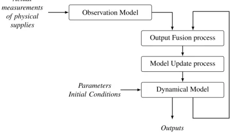
Dynamical Model Model Update process Output Fusion process Observation Model Outputs Actual measurements of physical supplies Parameters Initial Conditions
Fig. 1: Conceptual scheme of the data assimilation framework with the 3 main blocks. Adapted from13,14
traffic. Methods that use both model outputs and observed data are known as Data Assimilation (DA) methods. When new traffic data become available, traffic states are estimated based on the model states and the observed states, and the traffic model is updated accordingly.
In traffic, according to3, the DA problems have been addressed with Kalman filters extensions following the sem-inal work of Kalman4. They have been adressed with analytic extensions of the Kalman filter such as the Extended Kalman Filter (EKF)5, the Unscented Kalman Filter (UKF)6or the Mixture Kalman Filter (MKF)7. Other works lay on replications such as the Ensemble Kalman Filter (EnKF)8or the Particle Filter (PF)9. KF-based DA methods as-sume that the traffic model is linear, or at least differentiable. Several works aimed to use a KF method associated with a Eulerian LWR model: the Cell Transmission Model10. More recently, DA was explored within a Lagrangian-Space traffic model with both loop data11 and probe data12. These methods do not take into account model or observation errors. The aim of this work is to develop a DA method based on a Lagrangian-Space model that takes into account errors. The conceptual scheme of the development is based on13,14and is illustrated in Figure 1.
The paper is organized as follows. Section 2 introduces the dynamical traffic model used in the DA scheme. Section 3 introduces the output fusion analytic formulations and model update. Finally, Section 4 presents the results of the method on a straightforward application.
2. The LS-LWR model with error propagation
The Lighthill-Whitham-Richards (LWR) model was introduced in15and16to describe the dynamic of traffic stream. It consists in a conservative relation and a fundamental diagram. Originally, the LWR model were used considering Eulerian variables like the densityk, the flowqand the speedv. The Lagrangian-Time representation was proposed in the 90s, where the traffic variables provide time-position of individual vehicles, with a given time frequency.(see17). More recently, Lagrangian-Space (LS) representation has been proposed, (see18,19), where traffic variables provide passing time of vehicles at fixed locations on the network. The LS representation has proved to be well suited for assimilating data from inductive loop detectors11.
For the LS representation, the traffic model is solved in the (n,x) coordinates, wherendenotes the index of the vehicles andxthe space. The LS-LWR model follows the Hamilton-Jacobi theory, where the Hamilton-Jacobi partial derivative equation is derived from the conservation law:
∂xT = 1
Here, V is the flow speed, and the headwayh is denoted by its partial derivative formulation : ∂nT. The pace (inverse of speed) and the headway are related following an empirical convex relation: the fundamental diagram, considered as triangular in the remainder of the paper. The solution of the model provides the passing time of vehicle nat locationx:
T(n,x)=maxT(d)(n,x),T(s)(n,x) (2)
, whereT(d)(n,x) andT(s)(n,x) are the demand and supply terms, respectively.
For further details on the calculations see18and11. In the error-free formulation, all the passing times are computed with purely deterministic variables. Model errors come from errors on the parameters and the initial and boundary conditions. Model parameters are supposed to be distributed following Gaussian distributions. Besides, those con-siderations were legitimated by empirical studies on traffic stochasticity20. The outputs errors are not Gaussian. A previous work21enabled to propagate the errors to the outputs errors with Gaussian mixtures. A Gaussian mixture is defined as a convex combination ofJGaussian components. The notation of a passing time in the model with error propagation is the following:
T(n,x)=hnπ(T(nj),x), µ(T(nj),x), σ(T(nj),x)oi
1≤j≤J (3)
whereπ(T(nj),x),µ(T(nj),x)andσ(T(nj),x)are respectively the weight, the mean and the standard deviation of thejth compo-nent of the Gaussian Mixture.
3. Output Fusion and Model Update
The observation model consists in observed passing times of vehicles detected by the inductive loop detectors. Observation errors are supposedly Gaussian, which gives:
To(n,x)=nµTo(n,x), σTO(n,x)
o
(4) where µTO(n,x) denotes the mean and σTO(n,x) the standard deviation of the observed passing time distribution. According to22, the assimilated statesTa(n,x) follow a Gaussian Mixture distribution with the same number of com-ponentsJ. The aim of the method is to estimate the weightπ(Tj)a(n,x), the meanµ
(j)
Ta(n,x)and the standard deviationσ
(j) Ta(n,x) of the jth component of the assimilated state. The multi-component Kalman gain is introduced in order to reduce the mathematical formulation. Kj= σ(j) Tf(n,x) 2 σ(j) Tf(n,x) 2 + σTo(n,x)2 −1 (5) The following equations correspond respectively to the weight, the mean and the standard deviation of the jth component of the distribution of the assimilated state.
π(j) Ta(n,x)= π(j) Tf(n,x)× N(µTo(n,x), µ (j) Tf(n,x),(σ (j) Tf(n,x)) 2+(σ To(n,x))2) PM m=1π (m) Tf(n,x)× N(µTo(n,x), µ (m) Tf(n,x),(σ (m) Tf(n,x)) 2+(σ To(n,x))2) (6) µ(j) Ta(n,x) =µ (j) Tf(n,x)+K (j) µTo(n,x)−µ(j) Tf(n,x) (7) σ(j) Ta(n,x) 2 =(1−K(j))σ(Tj)f(n,x) 2 (8) Note thatNdenotes the Gaussian density function such as:
N(X,M,(Σ)2))= √1 2πΣexp −1 2 (X−M)2 (Σ)2 ! (9) The model state is then updated according to the assimilated state. Indeed, the sequential data assimilation is activated as new observed data are available. The model update ensures that the vehicles count and the traffic regime both remain consistent with the assimilated traffic states. During the update process, vehicles can either be added, deleted, delayed or advanced11.
4 A. Clairais et al./Procedia Computer Science 00 (2018) 000–000 ENTR Y EXIT 1000m 1000m 1000m 1000m 4000m N0 N1 N2 N3 N4
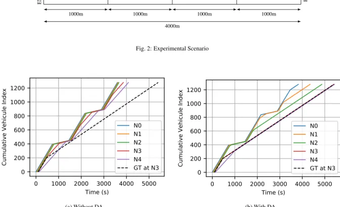
Fig. 2: Experimental Scenario
0
1000 2000 3000 4000 5000
Time (s)
0
200
400
600
800
1000
1200
Cumulative Vehicule Index
N0
N1
N2
N3
N4
GT at N3
(a) Without DA0
1000 2000 3000 4000 5000
Time (s)
0
200
400
600
800
1000
1200
Cumulative Vehicule Index
N0
N1
N2
N3
N4
GT at N3
(b) With DA Fig. 3: Comparison in terms of Cumulative Vehicle Index through simulation4. Illustration
The proposed data assimilation framework is tested on an experimental network composed of 4 consecutive cells where boundaries are numbered fromN0 toN4 (see Figure 2). The ground truth consists in the results of a mesoscopic LWR model23, designed so that a congestion starts and propagates fromN4 toN0 during the scenario. A loop detector is supposedly deployed atN3, which collects noised passing times (standard deviation of 0.5s), which constitute the observations.
Then boundary conditions of the experiment scenario differs from the ground truth (GT) scenario: the outflow capacity of the network has been voluntarily increased. Two simulations will be examined, without DA and with DA, based on two indicators: Cumulative Count Curves(CCC), also known as N-curvesfor flow analysis and the shockwave analysis;Travel Timesto complete with the analysis the propagation of errors/uncertainties through the network.
(i) Cumulative Count Curves. A cumulative count curve represents the cumulative vehicle index with respect to the
time at a given position on the network. CCC are plotted for successive positions (without source or sink in between). CCC is the raw output of the LS-LWR model. The performance of the proposed DA framework is illustrated, without DA on Figure 3a, and with DA on Figure 3b. In Figure 3a, three shockwaves can be observed: starting fromN4, they respectively reachN3 at around 500s, 1950s and 3300s. However, no shockwave is observed at boundariesN2−0, unlike the ground truth scenario. In Figure 3b, a shockwave can be observed, which propagates backward fromN3 (450s) toN0 (3500)through nodesN3. This scenario matches the observations at boundaryN3, and traffic states are properly propagated upstream. We conclude that the proposed DA framework enables to properly update the passing
0
500 1000 1500 2000 2500 3000
Time of entrance (s)
0
200
400
600
800
1000
1200
Travel Time (s)
Without DA
With DA
GT
(a) Means of the Travel Times
0
500 1000 1500 2000 2500 3000
Time of entrance (s)
0
2
4
6
8
10
12
14
Travel Time Std. Deviation (s)
With DA
Without DA
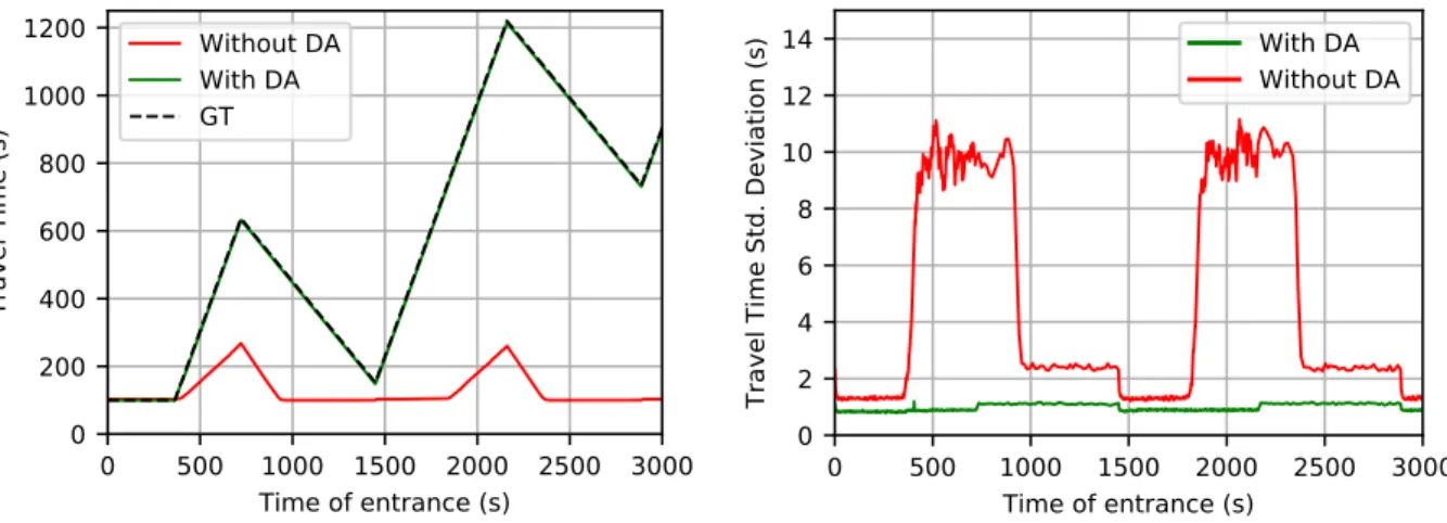
(b) Standard Deviation of the Travel Times Fig. 4: Comparison in terms of Travel Times through simulation
times at loop sensor locations, and shockwaves are properly propagated through the area of the network where no sensor is located.
(ii) Travel Times. In Figure 4a, travel times betweenN0 andN3 are illustrated with respect to the time.
Without DA, two congestion patterns are observed, between 400s and 800s; and then between 1300s and 2300s, but delays are significantly lower than delays from the ground truth. As expected, the congestion pattern is modified with DA. The travel times are consistent with travel times from the ground truth scenario. It should be noted that DA allow for the tracking errors on traffic state, which is illustrated in Figure 4b. Standard deviations of the travel time are plotted with respect to time. Errors remain low when the traffic is free-flowing, and they are greatly amplified during congestion (by a factor of nine times in this scenario) which is consistent with previous observation21.
5. Conclusion
The paper proposes a new DA framework based on a Lagrangian-Space LWR model with errors propagation. It consists in several steps. First, the model propagates traffic states and errors in time and space and provides passing times of vehicles at fixed location. The errors are considered distributed following Mixture of Gaussian distributions. In parallel, an observation model provides noised passing times of vehicles at a fixed locations of the network. Then an output fusion method has been proposed, to mix traffic states from the model with observed traffic states. Finally, the model is updated to ensure that the number of vehicles assimilated agree with the observations.
The proposed framework enables to propagate traffic states to locations with no observations. When boundary conditions are unknown or flawed, DA enables to update and propagate reliable traffic state through the network. Uncertainties are lower with DA than without, which paves the way for more reliable operational indicators.
References
1. Laharotte, P.A., Billot, R., Faouzi, E., Rakha, H.A., et al. Network-wide traffic state prediction using bluetooth data. In:Transportation Research Board 94th Annual Meeting; 15-3022. 2015, .
2. Elfaouzi, N.E.. Nonparametric traffic flow prediction using kernel estimator. In: Internaional symposium on transportation and traffic theory. 1996, p. 41–54.
3. Blandin, S., Couque, A., Bayen, A., Work, D.. On sequential data assimilation for scalar macroscopic traffic flow models. Physica D: Nonlinear Phenomena2012;241(17):1421–1440.
6 A. Clairais et al./Procedia Computer Science 00 (2018) 000–000
5. Wang, Y., Papageorgiou, M.. Real-time freeway traffic state estimation based on extended kalman filter: a general approach.Transportation Research Part B: Methodological2005;39(2):141–167.
6. Mihaylova, L., Boel, R., Hegyi, A.. An unscented kalman filter for freeway traffic estimation.IFAC Proceedings Volumes2006;39(12):31– 36.
7. Chen, R., Liu, J.S.. Mixture kalman filters.Journal of the Royal Statistical Society: Series B (Statistical Methodology)2000;62(3):493–508. 8. Evensen, G.. The ensemble kalman filter: Theoretical formulation and practical implementation.Ocean dynamics2003;53(4):343–367. 9. Liu, J.S., Chen, R.. Sequential monte carlo methods for dynamic systems. Journal of the American statistical association1998;
93(443):1032–1044.
10. Tamp`ere, C.M., Immers, L.. An extended kalman filter application for traffic state estimation using ctm with implicit mode switching and dynamic parameters. In:Intelligent Transportation Systems Conference, 2007. ITSC 2007. IEEE. IEEE; 2007, p. 209–216.
11. Duret, A., Leclercq, L., El Faouzi, N.E.. Data assimilation using a mesoscopic lighthill–whitham–richards model and loop detector data: Methodology and large-scale network application. Transportation Research Record: Journal of the Transportation Research Board2016; (2560):26–36.
12. Duret, A., Yuan, Y.. Traffic state estimation based on eulerian and lagrangian observations in a mesoscopic modeling framework. Trans-portation Research Part B: Methodological2017;101:51–71.
13. Kalnay, E..Atmospheric modeling, data assimilation and predictability. Cambridge university press; 2003.
14. Talagrand, O.. Assimilation of observations, an introduction (gtspecial issueltdata assimilation in meteology and oceanography: Theory and practice).Journal of the Meteorological Society of Japan Ser II1997;75(1B):191–209.
15. Lighthill, M.J., Whitham, G.B.. On kinematic waves. ii. a theory of traffic flow on long crowded roads.Proceedings of the Royal Society of London A: Mathematical, Physical and Engineering Sciences1955;229(1178):317–345. doi:10.1098/rspa.1955.0089.
16. Richards, P.I.. Shock waves on the highway.Operations research1956;4(1):42–51.
17. Newell, G.F.. A simplified car-following theory: a lower order model.Transportation Research Part B: Methodological2002;36(3):195–205. 18. Laval, J.A., Leclercq, L.. The hamilton–jacobi partial differential equation and the three representations of traffic flow. Transportation
Research Part B: Methodological2013;52:17–30.
19. Leclercq, L., Laval, J.A., Chevallier, E.. The lagrangian coordinates and what it means for first order traffic flow models. In:Transportation and Traffic Theory 2007. Papers Selected for Presentation at ISTTT17. 2007, .
20. Duret, A., Buisson, C., Chiabaut, N.. Estimating individual speed-spacing relationship and assessing ability of newell’s car-following model to reproduce trajectories.Transportation Research Record: Journal of the Transportation Research Board2008;(2088):188–197. 21. Clairais, A., Duret, A., El Faouzi, N.E.. Error propagation in traffic modelling: Solutions for the mesoscopic lwr model 2017;Technical
Paper, IFSTTAR.
22. Sondergaard, T., et al. Data assimilation with gaussian mixture models using the dynamically orthogonal field equations. Ph.D. thesis; Massachusetts Institute of Technology; 2011.
23. Leclercq, L., Becarie, C.. Meso lighthill-whitham and richards model designed for network applications. In: Transportation Research Board 91st Annual Meeting; 12-0387. 2012, .