Karoo Array Telescope site shielding : laboratory, computational and multi-copter studies

(1)

Laboratory, Computational and

Multi-copter Studies

by

Hardie Pienaar

Dissertation presented for the degree of Doctor of

Philosophy in Engineering in the Faculty of Engineering at

Stellenbosch University

Supervisors: Prof. H. C. Reader Prof. D. B. Davidson December 2015

(2)

Declaration

By submitting this dissertation electronically, I declare that the entirety of the work contained therein is my own, original work, that I am the sole author thereof (save to the extent explicitly otherwise stated), that reproduction and publication thereof by Stellenbosch University will not infringe any third party rights and that I have not previously in its entirety or in part submitted it for obtaining any qualification.

2015/9/1

Date: . . . .

(3)

Abstract

Karoo Array Telescope Site Shielding: Laboratory,

Computational and Multi-copter Studies

H. Pienaar

Department of Electrical and Electronic Engineering, University of Stellenbosch,

Private Bag X1, Matieland 7602, South Africa.

Dissertation: PhD (E&E) December 2015

The Northern Cape in South Africa has been chosen to host the Square Kilo-metre Array (SKA) due to the area’s overall radio quietness. As part of the supporting systems for the Karoo Array Telescope (KAT), a processing build-ing has been constructed on the site. With the Karoo Array Processbuild-ing Build-ing (KAPB) now in place, investigatBuild-ing the radio frequency interference (RFI) of the building has become a high priority. If successful, understanding of RFI propagation on-site will shape policies and contribute to the sustainability of on-site radio quietness. This dissertation focuses on understanding the shield-ing and propagation characteristics of both the KAPB buildshield-ing, as well as a man-made soil berm. On-site measurements, scale models and computational models will be used to investigate the local electromagnetic environment. Ad-ditionally, a Multi-copter vehicle is developed to support on-site measurement campaigns. Using data measured on-site it was possible to develop empirical models for local shielding estimations. It was found that the shielding perfor-mance of the berm was primarily affected by diffraction. Also, the developed computational model makes it possible to investigate alternative terrestrial structures. The work done in this dissertation will permit off-site analysis of propagation over terrestrial structures. Moreover, the development of a Multi-copter measurement platform creates more efficient metrology. Finally, empirical models are designed so that shielding budgets can be calculated for noise sources to the nearest receivers.

(4)

Uittreksel

Karoo Array Teleskoop Omgewing Beskerming:

Laboratorium, Rekenaar Modellering en Multi-kopter

Studies

H. Pienaar

Departement Elektriese en Elektroniese Ingenieurswese, Universiteit van Stellenbosch,

Privaatsak X1, Matieland 7602, Suid Afrika.

Proefskrif: PhD (E&E) Desember 2015

Die Noord Kaap in Suid Afrika is gekies om ‘n gedeelte van die Square Ki-lometre Array (SKA) te huisves. Die besluit is gedeeltelik gemaak as gevolg van die skoon radio omgewing in die Noord Kaap. ‘n Ondergrondse gebou, ge-naamd die Karoo Array Processing Building (KAPB), is gebou as deel van die ondersteunende infrastrukture van die Karoo Array Telescope (KAT). Met die oprigting van die Karoo Array Processing Building (KAPB), het dit belang-rik geraak om radio frekwensie steuring (RFI) te ondersoek. Indien die studie suksesvol is, sal die begrip van RFI voortplanting in die omgewing help om be-leid te vorm ten opsigte van die volhoubaarheid van die skoon RFI omgewing. Hierdie proefskrif fokus op die verstaan van beskermings verm¨oe van beide die KAPB gebou en die mensgemaakte keerwal asook plaaslike radio frekwensie voortplantings karakteristieke. Metings geneem in hierdie area, skaalmodelle sowel as numeriese elektromagnetiese modellering (CEM) is gebruik om die plaaslike elektromagnetiese omgewing te ondersoek. Verder is ’n Multi-kopter platvorm ontwikkel vir die ondersteuning van metings veldtogte. Deur gebruik te maak van gemete data wat geneem is in die area, kon empiriese modelle ont-wikkel word wat gebruik is om die plaaslike RFI beskerming te beraam. Daar is gevind dat die beskerming van die heuwel hoofsaaklik geaffekteer word deur die diffraksie daaroor. ’n CEM model is ook ontwikkel om die ondersoek van ander heuwelagtige strukture moontlik te maak. Die werk in hierdie proef-skrif sal dit moontlik maak om analise, weg van die Karoo omgewing te doen. Addisioneel, het die ontwikkeling van ’n Multi-kopter platvorm dit moontlik gemaak om metings vinniger te doen. Die uiteinde is dat empiriese modelle dit

(5)

UITTREKSEL iv

moontlik maak om ’n beskermings verm¨oe begroting uit te werk vir ’n geraas bron tot die naaste MeerKAT ontvanger.

(6)

Acknowledgements

I would like to express my sincere gratitude to the following people: My family who supported and inspired me.

Anneke Stofberg for her dedicated support through all, especially the hard, phases of this project.

Prof H. C. Reader for his wholehearted guidance through the project as well as his passionate teachings in EMC. His impromptu lessons in language will shape my English for years to come.

Prof D. B. Davidson for his valuable guidance and inputs during the last year of my PhD.

Braam Otto and Paul van der Merwe from MESA for their support in my Multi-copter and dielectric measurement efforts. They kept their belief, even in times when things started flying away.

Simon Norval for arranging and making most of the measurements in this dissertation possible.

Wessel Croukamp for his support and advice in all things mechanical. Johan Frank for giving me the confidence and guidance to pilot a Multi-copter for the first time.

The past and present members of the EMRIn group: Matthew Groch, Antheun Botha, Nardus Mathyssen, Stefan Combrink, Joely Andriambe-loson for a place to share thoughts and ideas as well as their contribution to all the interesting moments in room E212.

This project was funded by SKA South Africa and CHPC.

(7)

ACKNOWLEDGEMENTS vi

Figure 1: Photo of our group during the last Karoo measurement campaign discussed in this work. From top left: Stephan Combrink, Simon Norval, Carel van der Merwe, Paul van der Merwe, Nardus Mathyssen, Braam Otto. From bottom left: Hardie Pienaar, Antheun Botha, Gideon Wiid.

(8)

List of Figures

1 Photo of our group during the last Karoo measurement campaign

discussed in this work. From top left: Stephan Combrink, Simon Norval, Carel van der Merwe, Paul van der Merwe, Nardus Math-yssen, Braam Otto. From bottom left: Hardie Pienaar, Antheun Botha, Gideon Wiid. . . vi

1.1 Perspective from the top of the 13 m high berm facing towards

Losberg. The KAPB and assembly shed can be seen to the left. The core of MeerKAT is located on the opposite side of Losberg. Photo by Dr P. G. Wiid. . . 2

2.1 Photo showing three of the seven KAT-7 telescope dishes. KAT-7

is the precursor to MeerKAT. . . 7

2.2 Diagram showing how the geometry of the wire example has been

approximated into linear segments. The left side is the original problem where currents could exist in arbitrary orientations on the wire surface. On the right, currents are constrained onto the axial direction of the wire. . . 9 2.3 Schematic of the transmission line example. The transmission line

itself has been discretised into lumped-element components. . . . 12

2.4 Diagram illustrating a 2D Yee grid for the transmission line exam-ple. Here the staggering of the voltage and current points can be seen. The variables involved in calculating a single voltage point are also demonstrated. . . 13 2.5 Illustration of Huygens principal. A source emits a wavefront into

a wedge obstacle. The third wavefront demonstrates how energy is

diffracted into the shadowed region by using Huygens principle. . 17

2.6 Photo of LS of SA using their Multi-copter platform for a

mea-surement. Receiver and computer equipment are mounted on the bottom of the vehicle with the antenna secured to a fixture between two of the motor arms. . . 19

2.7 Photo of the IEIIT Group Multi-copter during an array scanning

measurement. Dipole antenna and tone generator can be seen mounted on its underside. . . 19

(12)

LIST OF FIGURES xi

2.8 Photo of a Multi-copter being used at the University of Nijmegen. The antenna, in this case, has been placed away from the vehicle. Photo was taken from Krause [48]. . . 20 2.9 An illustration of a material subject to an applied E-field. After [52]. 22 2.10 Parallel plate illustration. After [52]. . . 22 2.11 Free-space measurement system. . . 24 2.12 X-band waveguide measurement system during a through

calibra-tion. Material holders and calibration sections can be seen in the background. . . 25 2.13 Coaxial probe system. . . 25

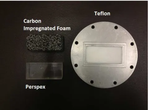
3.1 Photographs of the S-Band and X-Band waveguide measurement

sets including calibration standards and sample holders. . . 28 3.2 S-Band samples with Teflon already fitted into the sample holder.

Teflon and Perspex will be used for reference measurements. . . . 29

3.3 S-Band waveguide time-gated S-parameters. . . 31

3.4 X-Band waveguide time-gated S-parameters. . . 31

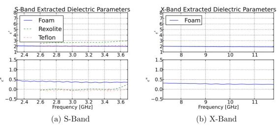
3.5 S-Band and X-Band permittivity extracted with the improved NRW

algorithm. . . 32 3.6 Offline calibration using a load, short and offset short. At this point

the short is measured at z = 0 with an absorbing foam block, also the load, behind it. . . 34

3.7 Model of S-parameter systematic errors. . . 35

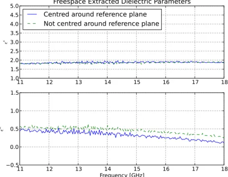
3.8 Offline calibrated measurement of the foam on the free-space system. 36

3.9 Calibrated S-parameter measurements of the foam with reference

planes shifted. . . 36 3.10 Root combination minimum error plot at 11.6 GHz. This plot solves

the left-hand side of Eq. 3.3.5. . . 37 3.11 Free-space extracted parameters of the foam. A slight ripple is

present in the extraction due to calibration simplifications. . . 38

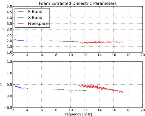
3.12 Dielectric data over all of the three measurement campaigns. . . . 40

3.13 Fitted polynomial and log trend. . . 40

4.1 Diagram of the metallic plate used for scale measurements. The

antennae are located at each end of the plate, with the aluminium

mounted on a wooden base for extra mechanical support. . . 44

4.2 Diagram (left) and photo (right) of the fat monopole antenna,

mounted on the metallic plate, with its feeding connector on the bottom side of the structure. The antenna was machined out of brass material. . . 44

4.3 Photo of the scale-model measurement setup inside the anechoic

room. . . 45 4.4 Scale model, without dielectric, measured outside of the anechoic

(13)

LIST OF FIGURES xii

4.5 Antenna feed mesh in CST MWSR

. Here it can be seen how all of the detailed features have been meshed. Additionally the connector dielectric section has been given extra mesh cells to account for its shorter wavelength. . . 46

4.6 Computational models constructed in CST MWSR

. A simulation with and without the dielectric was used for the measurement com-parison. The dielectric and the non-dielectric measurement con-tained respectively 227 and 190 million mesh cells. . . 47

4.7 Both measurement and simulated scenarios, without the dielectric

(a), and with the dielectric (b), are compared. A more efficient infinite approximation is also shown in (a). . . 47 4.8 Illustrating how rays are diffracted on a thin PEC serration with

an oblique angle. To illustrate the optimisation case, a 2D version is also shown. . . 49 4.9 Diffracted ray comparison for an optimised and non-optimised plate,

using a simplified GTD approximation. The dot at the top of the plate represents the transmitting antenna while the surrounding square indicates the zone that is optimised to be free of diffrac-tions. In the non-optimised case, red rays indicate rays that have passed through this zone. . . 50 4.10 Testing of the serrated plate compared to the infinite case using

CST MWSR

. In (a) the S21 coupling is compared showing good

agreement between the time-gated-serrated measurement and the actual infinite case. The time domain received wave can be seen in

(b), showing the direct and reflected waves. TG - Time-gated. . . 51

4.11 Constructed serrated plate with its non-dielectric measurement. Here the serrated time-gated measurement is compared to a full infinite plate CST MWSR

simulation. . . 52

4.12 FEKOR

PEC half-space compared to infinite CST MWSR

simu-lation in (b). The two antennas can be seen on both sides of the image, on top of the infinite PEC halfspace. . . 53

4.13 FEKOR

mirrored simulation including dielectric. Results here are compared to quasi-infinite measurements. . . 54 4.14 Full berm simulation with antenna 50 m away. The berm and

antenna were both mirrored around the ground plane to make

RL-GO in FEKOR

possible. . . 55 4.15 Simulation of a vertical plane, showing the E-field through the

cen-tre of the berm at 260 MHz. The source used in this simulation is the simple resonant monopole on the ground. The solution is not valid inside dielectric volumes. Therefore, the area that contained the berm is left blank. . . 55

4.16 Fresnel integral as a function of v. This graph was taken from

(14)

LIST OF FIGURES xiii

4.17 Simulated shielding, with a monopole on the ground, 50 m in front of the berm at 260 MHz. . . 57 4.18 Shielding simulations to a nearby MeerKAT location for the berm

at heights of 4, 10 and 40 wavelengths. The border from the line-of-sight to the shadowed regions are indicated by white lines. The KAPB location is roughly outlined by dashed lines in the figures. This marked volume is what is used to calculate figures of merit called ASE and MSE. . . 58 4.19 Simulated 2D planes using the mirrored berm approximation. The

vertically polarised source is located at the position of receiver M60 15 m off of the ground, 5 km away. The planes illustrate the abso-lute electric field diffracted over and around the obstacle. . . 59 4.20 The same simulation configuration as in Fig. 4.19 with shed

struc-tures added. . . 60 4.21 Berm shielding effectiveness in KAPB area to MeerKAT receiver

M60 at 260 MHz. In this case, a large PEC shed structure has been added, causing diffraction into the shielded area. . . 60 4.22 Comparison of our PEC, PMC ground cover approximating

real-earth using a 2D FDTD model. Both the diffraction (non-grazing angle) and shielding (grazing angle) scenarios are tested. . . 61

4.23 Diffraction flight path simulations at 50m and 200m. . . 63

4.24 Horizontal plane measurement made by LS of SA compared to the

FEKOR

model. Measurements directly behind the berm are mostly in the noise floor. However, the propagation around the berm is still informative. . . 63 4.25 Berm loss-tangent parameter study. The loss-tangent was varied

initially by only 20% up and down. Due to the insignificant change, the loss-tangent was further changed by an order of magnitude. This shows how diffraction over the berm converges with an increase in conductivity. . . 64

5.1 Multi-copter CAD model compared to a photo of its realised

coun-terpart. Plastic parts were 3D-printed while metallic structure parts were obtained from a local hardware store. . . 67

5.2 Photo and diagram of flight electronics. In (b), the connections

between the different electronics can be seen. . . 68

5.3 Photos of the RFM22B transceiver module. In (b), the transceiver

is shown on its daughter board attached to the Raspberry Pi. . . 70

5.4 Software diagram of the logging script running on the

Raspberry-Pi. This python script is initialised before each flight and is only terminated after the flight has ended. . . 71 5.5 The calibration file used during post-processing for a pamp

re-ceiver pair. This file was created using a known signal-generator as an input while logging the output of the receiver. . . 71

(15)

LIST OF FIGURES xiv

5.6 System diagram of the real-time transient analyser. . . 72

5.7 Front-end switchable filter-bank configuration. . . 73

5.8 Photo of the digital board containing the FPGA, ADC and clock

generator. . . 73 5.9 Photo of the unshielded switch-able filter bank. Filters are

imple-mented using lumped elements. . . 74 5.10 Photo showing the layout of the dual antenna configuration. In

(b), the isotropic antenna pattern formed by an idealised dual-configuration can be seen. . . 75 5.11 A photo in-flight showing the grounded-copper shield enclosure.

The compass and GPS due to the nature of their operation are still

placed on the top of the cube. Photo was taken by Dr. P. G. Wiid. 76

5.12 The loading profile of the monopole can be seen in (a). In (b) a picture of the initial simulation model, used in CST MWSR

, can be seen. One half of the leg here is removed to reveal the antenna with its loaded elements. . . 77 5.13 Image of the full Multi-copter CEM model. Here the simulated

input reflection of the antenna is compared to its measured equivalent. 78 5.14 Realised gain of Multi-copter antennas on a constant phi cut. Cut

locations were chosen to align with the deepest nulls of each pattern. During measurement extraction, the data from the antenna with the highest realised gain will be used. Here the difference with increasing frequency can be seen. . . 78 5.15 Multi-copter mounted on the near-field scanning device. The

high-lighted (white line) is the active antenna during the measurement. 79 5.16 Measured 2D theta/phi antenna patterns. Data transformed to

far-field from a near-field scanning measurement. . . 80

5.17 Simulated 2D antenna patterns using CST MWSR

. . . 80

5.18 Measurement of Multi-copter RFI signature using a reverberation chamber. The measurement can be seen in (a) with a photo of the Multi-copter in the chamber in (b). . . 82 5.19 A simplified schematic of the Multi-copter illustrating the

clean-room dirty-clean-room concept. The receiver is shielded from the internally-generated RFI, illustrated in grey. . . 83 5.20 De-embedding measurements using receiver calibration data and

simulated antenna patterns. Deviation between the fully extracted data in (c) is a result of slight simulation deviations together with the uncertainty of the principle incoming signal’s direction. . . 87

6.1 Contemporary photo of the KAPB, dark roof, taken from the top

of Losberg. The berm and the assembly shed can be seen on the left and right of the KAPB respectively. Photo was taken by Dr P. G. Wiid. . . 92

(16)

LIST OF FIGURES xv

6.2 Diagram illustrating how shielding, S, is calculated around the

KAPB, at points x, while transmitting from different rooms, r, inside the building. . . 93

6.3 Shielding measurement of the KAPB at three discrete frequencies.

Ground measurements were done using a hand-held spectrum anal-yser while measurements at 10 m height were accomplished using the Multi-copter platform. The measurements can be compared to the diagram in (d) for a sense of orientation. . . 94

6.4 Shielding measurement along the berm-side of the KAPB compared

to ground measurements on top of the berm. Vertical lines indicate the start and stop of the KAPB berm-side wall. . . 95

6.5 Vertical-plane signal strength graph, measured between the KAPB

and berm. The diagram in (b) gives an overview of how the mea-surement was planned. . . 96

6.6 Vertical shielding measurement, on the berm side of KAPB. This

plot shows, at two discrete frequencies, how shielding tends to de-crease with height. A diagram showing how the measurement was conducted can be seen in (b). . . 97

6.7 Minimum shielding vs frequency trend extracted from polar

pat-tern shielding graphs. A square fit was used to approximate the

measurements, which can now be used as an analytical tool. . . . 98

6.8 Ground loss measurement compared to the simple ground loss model

at two different heights. A free-space prediction can also be seen for comparison. A schematic in (b) gives an overview of the mea-surement setup. . . 99

6.9 A diagram of the berm and KAPB environment. Here the location

of the antenna can be seen. A region called sampled space was

measured to obtain the vertical-plane measurements in Fig. 6.10. 100

6.10 Vertical plane measurements of a noise source transmitting over the berm. At the two discrete frequencies diffraction is seen in the shadowed region of the berm. . . 101 6.11 A diagram of the diffraction measurements. Here the two

measure-ment locations along with the transmitting position, on the far side of the berm, can be seen. Three discrete frequencies were measured at each location. . . 102 6.12 Different diffraction model geometries used in the characterisation

of the berm. These models range from infinitely-thin PEC knife edges to finitely conducting wedges. . . 103 6.13 Comparison between real measurement and model configurations

seen in Fig 6.12. Measurement was taken at 550 MHz 200 m behind berm. . . 103 6.14 Comparisons between measurement and calibrated model for berm

diffraction. These graphs represent two different positions as well as two different frequencies behind the berm. . . 104

(17)

LIST OF FIGURES xvi

6.15 Google Earth satellite map showing the location of the KAPB and berm relative to the nearest MeerKAT receiver. . . 106 6.16 Shielding to nearest MeerKAT receiver (M59) from inside KAPB,

outside KAPB and outside KAPB not shielded by the berm. Height for the outside RFI positions were kept at 2 m high 70 m from the foot of the berm. In (b) the maximum allowable signal transmitted,

from inside the KAPB, can be seen graphed using (a). . . 107

6.17 Comparison between the computational models and Multi-copter measurements for a diffraction flight 200 m behind berm at 900 MHz.110 6.18 Geometry used to calculate when the PEC reflections affect the

simulation. . . 111 6.19 Comparison between model predictions and on-site measured data

for the three main scenarios. Dashed and solid lines respectively illustrate the difference between using the two-ray or Egli model for ground propagation. . . 112 6.20 Received level at M59 and M60 receivers using the measured

emis-sions in the KAPB, translated using the developed empirical mod-els. An upper and lower bound for shielding were calculated using the models from this work. SARAS levels are added to asses RFI severity. . . 113 A.1 S-Band measurements made over multiple occasions to illustrate

repeatability of measurements. . . 120 A.2 X-Band measurements made over multiple occasions to illustrate

repeatability of measurements. . . 121 A.3 Comparison between typical and improved NRW code. As a result

of choosing the incorrect root, the extraction deviates. The point at which this happens is illustrated as the wrapping point in the phase graph. . . 121 B.1 Amplitude in dB of the radiation pattern in the E-plane along the

z-axis for a frequency of 13.5 GHz. Difference between contours are 2dB with a -2dB contour in the middle. . . 125 B.2 Measured standards used in offline calibration. . . 126

B.3 Calculated error terms used to calibrate measurements offline. . . 127

B.4 Root combinations found over frequency for minimum error using Eq. 3.3.5. . . 130 B.5 Root combinations error over frequency. . . 130 B.6 Root combination minimum error plot at 12.39 GHz. This plot

solves the left-hand side of Eq. 3.3.5. . . 131 B.7 Root combination minimum error plot at 18 GHz. This plot solves

(18)

LIST OF FIGURES xvii

C.1 Russouw Probe with its calibration standards. A short on the left

and matched load on the right. . . 137

C.2 Marais Probe with its calibration standards. From left; a short, matched load and a characterised open. . . 137

C.3 Samples used in coaxial probe measurements. From left; Foam material, Rexolite, Perspex and Teflon. . . 138

C.4 Extracted foam measurements using Rossouw probe. The influence of the material structure can be seen in the random deviations of the measurements.The dashed line indicates the waveguide mea-surement for the same band. . . 139

D.1 In (a), an illustration of variable edges used to build the optimised geometry. The first edge here is already fixed while the second edge is being varied to optimise its angle. Additionally, the discretisation of an edge to calculate diffraction interactions can be seen in (b). 142 D.2 Illustration of diffraction on a serrated plate. A simple non-optimised serration geometry was used, varying length of the vertexes. . . . 143

E.1 Daughter board schematic, drawn using KiCad [87]. . . 152

E.2 PCB design for the RFM22B daughter board. The PCB is respon-sible for connecting the transceiver module to the Raspberry-Pi. Additionally, an SMA connector for the antenna is supplied. . . . 153

E.3 Multi-copter far-field antenna patterns. These realised-gain pat-terns give an indication of the field at three discrete frequency points. Continued in E.4. . . 154

E.4 Multi-copter far-field antenna patterns. These realised-gain pat-terns give an indication of the field at three discrete frequency points.155 E.5 Specification sheet for the MT2216 (800 KV) dc-brushless motor [89].156 E.6 Electrical Specifications of the ZX60-P105LN+ from Mini-Circuits. 157 E.7 Performance Graphs of the ZX60-P105LN+ from Mini-Circuits. . 157

F.1 Photo showing the spark-gap on the 12 kV line. The LPDA re-ceiving antenna can be seen as the orange structure directed at the spark-gap. . . 167

F.2 Sparking measurement showing the broadband nature of the pulses extending to 400 MHz. A background measurement distinguishes the environment from sparking. . . 168

F.3 Root page . . . 169 F.4 Clock page . . . 170 F.5 ADC page . . . 171 F.6 FPGA page . . . 172 F.7 Power page . . . 173 F.8 Front Copper . . . 174

(19)

LIST OF FIGURES xviii

F.10 Inner layer 2 Copper . . . 175

F.11 Back Copper . . . 175

F.12 Silk screen . . . 176

F.13 Filterbank PCB Layout . . . 176

F.14 Filterbank schematic . . . 177

F.15 Spectrum plot with 50 Ω load connected to the input. . . 208

F.16 -12.5 dBm 90 MHz tone applied at input. . . 209

F.17 -22.5 dBm 90 MHz tone applied at input. . . 209

G.1 Multi-mode antenna placed in the middle of a large sports field aligned East to West. In this case, the Rat-race coupler was used to drive the antenna in its horizontal dipole mode. . . 210

G.2 E-plane dipole antenna measurement using Multi-copter compared to laboratory characterised data. Deviation in measurements are caused by the null region de-embedding of on-board antennas. . . 211

H.1 Diffraction measurements at two discrete points behind berm at 260 MHz. These measurements are compared to the calibrated knife-edge model. . . 213

H.4 Vertical-shielding measurements for the remaining three sides of the building. The berm side has been discussed in the text. . . 215

(20)

List of Tables

2.1 Brief comparison between the fundamental aspects of the discussed CEM codes. . . 8 2.2 Summary of different terrestrial propagation mechanisms at various

frequencies. . . 16

2.3 Examples of some near-earth propagation models. . . 17

2.4 Comparison table between three different dielectric measurement

methods used in this dissertation [53]. . . 26

3.1 Overview and comparison of S and X-band waveguide systems. . . 28

3.2 Comparison between known and measured values for Perspex and

Teflon. The reference values are both average values over their given frequency bands. . . 32

3.3 Calibration standard definitions for the free-space measurement

system. The measured traces for each standard will be named according toM1,M2 and M3. . . 34

3.4 Expressions for the error coefficient in the model seen in Fig. 3.7. 35

3.5 Lowest error root combinations uniqueness table . . . 38

3.6 Amount of linear test error for each order fit. . . 39

4.1 Frequencies on the scaled model compared to the full-size berm. . 42

4.2 Dimensions of the characterised foam block. . . 43

4.3 FOM results in the RoI for the 3D RL-GO and 2D boundary

inte-gral models. . . 59 5.1 A weight estimate of the Multi-copter with all of its systems on-board. 67 5.2 Brushless-dc motor specifications. This data is valid for an MT2216

900 KV motor at 11.1V on an 11x3.7 inch propeller. The rest of the data can be found from the manufacturer’s specification sheet in Appendix E.3. . . 68

6.1 Minimum shielding levels on the berm side of KAPB extracted from

Fig. 6.3. . . 97

(21)

LIST OF TABLES xx

A.1 Calibration Standards defined for S-Band Waveguide system in CalKit Manager. Using a short, offset short, thru and sliding load calibration. . . 119 A.2 Calibration class assignments defined for S-Band Waveguide system

in CalKit Manager. . . 119 A.3 Calibration Standards defined for X-Band Waveguide system in

CalKit Manager. Using a short, line and thru calibration. . . 120 A.4 Calibration class assignments defined for X-Band Waveguide

sys-tem in CalKit Manager. . . 120 C.1 Real permittivity of known materials, measured using coaxial probes.

Each measurement is repeated three times, each with a new cali-bration. . . 138 D.1 Coordinates for one-quarter of the optimised plate. . . 144

(22)

(23)

NOMENCLATURE xxii

Nomenclature

Abbreviations

ADC Analog-to-Digital Converter

AGA Astronomy Advantage Act

ALMA Atacama Large Millimetre/sub-millimetre Array

ASE Average Shielding Effectiveness

CAD Computer Aided Design

CEM Computational Electromagnetics

COTS Commercial Off-The-Shelf

EM Electromagnetic

EMC Electromagnetic Compatibility

ESC Electronic Speed Controller

FEM Finite Element Method

FDTD Finite Difference Time Domain

FIFO First In First Out

FOM Figure of Merit

FPGA Field Programmable Gate Array

GO Geometrical Optics

GTD Geometrical Theory of Diffraction

GPS Global Positioning System

HV High Voltage

KAPB Karoo Array Processing Building

KAT Karoo Array Telescope

LNA Low Noise Amplifier

LOS Line of Sight

LPDA Log Periodic Dipole Antenna

MoM Method of Moments

MSE Minimum Shielding Effectiveness

MUT Material Under Test

NRW Nicolson-Ross-Weir

PEC Perfect Electric Conductor

PLF Polarisation Loss Factor

PCB Printed Circuit Board

PMC Perfect Magnetic Conductor

PML Perfect Matching Layer

PO Physical Optics

RaTTy Real-time Transient Analyser

RC Remote Control

(24)

NOMENCLATURE xxiii

RFI Radio Frequency Interference

RoI Region of Interest

RSSI Receive Signal Strength Indicator

RL-GO Ray Launching Geometrical Optics

SARAS South African Radio Astronomy Service

SBC Single Board Computer

SE Shielding Effectivenesss

SERDES Serial/Deserializer

SKA Square Kilometre Array

SKASA Square Kilometre Array South Africa

SMA Sub Miniature version A

SPI Serial Peripheral Interface

TE Transverse Electric

TG Time Gate

TEM Transverse Electromagnetic

UHF Ultra High Frequency

UTM Universal Transverse Mercator

VHDL VHSIC Hardware Description Language

VHF Very High Frequency

VLA Very Large Array

VNA Vector Network Analyser

Constants

c 299792458 m/s

ǫ0 8.854×10−12 F/m µ0 4π×10−7 H/m

(25)

Chapter 1 Introduction

1.1 The SKA and RF propagation studies

The Square Kilometre Array (SKA) will be the world’s largest radio telescope upon completion. Currently in its pre-construction phase, implementation is planned to start in 2018 with early science possible in 2020. The project will be the world’s largest public science data undertaking with data rates reaching ten times more than current Internet traffic around the globe. The SKA will be completed in two phases, the first of which will contribute to around half of the projected one square kilometre collecting area. During phase two, the collecting area will surpass one square kilometre by some margin. Some of the key science goals are to: test the theory of relativity; discover how the universe with its stars and galaxies formed and evolved; answer questions about dark matter and dark energy; find the origin of cosmic magnetism; continue the search for extraterrestrial life and finally make discoveries that cannot at this point be foreseen.

SKA phase 1 is set to achieve a frequency range of 50 MHz up to 14 GHz which is split between the two host countries South Africa and Australia. Approximately a quarter of a million low-frequency aperture array antennas, covering 50 MHz to 350 MHz, will be built in the Murchison Valley of Australia (SKA1 LOW). The rest of the frequency band, 350 MHz to 14 GHz, will be surveyed using around 200 dishes located in the Karoo desert of South Africa (SKA1 MID).

SKA MID1 currently boasts an estimated baseline of 150 km. Resolution and sensitivity will be respectively four and five times higher than that of the Jansky Very Large Array. Survey speed will see a sixty times improvement over the latter telescope. Precursor telescopes are currently under construction to help us understand the necessary challenges. MeerKAT in South Africa and the MWA[1] and ASKAP[2] in Australia are playing a key role in helping us understand the difficulties ahead. SKA Phase 2 will see the expansion of the array into neighbouring African countries. Similar expansion is planned for

(26)

CHAPTER 1. INTRODUCTION 2

Figure 1.1: Perspective from the top of the 13 m high berm facing towards Losberg. The KAPB and assembly shed can be seen to the left. The core of MeerKAT is located on the opposite side of Losberg. Photo by Dr P. G. Wiid. the Australian components. Full completion would take around a decade with enabling technologies still needing further refinement [3].

In South Africa’s SKA developments, the Karoo has been chosen princi-pally for its pristine Radio Frequency (RF) Environment. With the construc-tion of Karoo Array Processor Building (KAPB), self-generated noise and its propagation into surrounding telescopes become a concern. This investigation seeks to quantify shielding effectiveness to nearby MeerKAT receivers from the KAPB site. Empirically-based propagation and shielding models will allow a stronger basis for qualifying on-site infrastructure in terms of its local radio frequency interference (RFI) emissions. As part of the KAPB construction, excavated earth was used to build a berm adjacent to the building. The ben-efits of this decision were twofold, lowering the cost of transporting the soil and using it as a shielding mechanism between the KAPB and the nearest MeerKAT receivers. A Multi-copter metrology vehicle was designed to facili-tate on-site measurement campaigns. Such a platform enables characterisation of the berm and KAPB (see Fig. 1.1) at different heights. In the case of the berm this allows measurements up to 100 m and thus makes it possible to investigate diffraction over a significant range. Apart from the empirical prop-agation tools, a verified computational model is created to allow exploration into more complex berm configurations. Such configurations could investigate different berm geometries as well as the addition of other on-site obstacles.

Previous work for on-site shielding includes:

• Characterising the absorption properties of the Karoo soil for cable-shielding studies [4].

• Investigating end-fire patterns from power-line sparking using a Multi-copter [5][6].

• Investigating shielding of soil structures using scale-model measurements [7].

• Time-domain studies using a real-time transient analyser and impulse

radiating antenna was used to investigate broadband propagation on the site area [8].

(27)

It is important to develop tools to expedite measurements. These on-site efforts are time-consuming and become more logistically involved as MeerKAT comes into operation. Therefore, this work has focussed on using these lim-ited measurement campaigns to build empirically-based propagation models, and a verified computational model, for off-site investigations. During these campaigns, a Multi-copter measurement platform considerably increased the possible investigations.

1.2 Dissertation objectives

The primary objective of this dissertation is to develop propagation models for the Karoo site as part of the campaign to study and minimise the effects of self-generated interference. The initial part of achieving this goal is the establishment of a practical computational model of the on-site berm using scale-model and full-scale measurements. To expedite and enhance on-site measurement capabilities, a Multi-copter measurement platform is designed. This vehicle will be employed for the full-scale propagation measurements as well as the KAPB shielding investigations. Finally, full-scale measurements will be used to compile a set of empirical propagation models that will char-acterise the severity of on-site RFI sources. The scope of this work will not include investigations into small-scale fading, ionospheric and atmospheric ef-fects, and long distance over-the-horizon propagation. This work will mainly focus on the local shielding-effectiveness characteristics of the KAPB site.

1.3 Contributions

The original contributions made in this dissertation include the following:

1.3.1 Development of a Multi-copter for RFI and

propagation studies

To expedite and enhance on-site measurement campaigns, a Multi-copter was designed and deployed specifically for radio-frequency interference and prop-agation studies. Measurements could be fully de-embedded from the vehicle due to a shielded configuration. This made characterisation of the on-board antennas reliable and facilitated the accurate de-embedding of data. The effect of the complex vehicle on the antenna system is circumvented in most other Multi-copter designs by using a decoupled directional antenna or only focussing on relative measurements while ensuring symmetry around the antenna. Ad-ditionally, an integrated dual-antenna configuration forming a quasi-isotropic antenna pattern implemented on the vehicle guaranteed a good degree of sen-sitivity irrespective of its orientation. The antennas formed an integral part of

(28)

the Multi-copter design to the point where they were embedded into its landing structures, making use of the surrounding dielectric material to achieve a lower minimum measurable frequency. The conductive shield simplified the electro-magnetic structure of the vehicle to the extent that fully verified simulations were possible. These simulations were used to generate patterns critical for the antenna de-embedding process. All of this contributed to a Multi-copter metrology vehicle with the capacity of doing accurate absolute measurements.

1.3.2 Study of berm shielding characteristics

The shielding characteristics of a real-world berm was studied using a com-putational model derived from laboratory scale measurements and in-field metrology. The simplified 3D computational model was verified using full-scale diffraction measurements. Using this model, shielding metrics could be derived for the 3D berm case. Previously this was only done for an infinite 2D approximation of the structure. It was found from this study that a berm only becomes effective after its height reaches around 10 wavelengths with an average shielding effectiveness of 10 dB. A minimum shielding level of 15 dB is found when the berm height reaches 40 wavelengths.

1.3.3 Compilation of simplified propagation models

based on on-site measurements

A set of simple propagation models for local on-site propagation was com-piled to analyse the severity of emission sources on near-lying receivers. This was made possible by using the large scale (100 m vertical) diffraction mea-surements to calibrate a simplified single knife-edge model for the berm. The shielding performance of the KAPB was characterised using the Multi-copter platform. Finally, ground loss models were tested using horizontal measure-ments at varying heights.

1.4 Layout of the dissertation

The dissertation will start with a literature review covering the background on topics encountered through the text. This will include information on the Square Kilometre Array South Africa (SKASA), radio frequency inter-ference, computational modelling, propagation, knife-edge modelling, Multi-copters and dielectric measurements.

Chapter 3 will focus on the broadband characterisation of a dielectric block. This chapter will make use of a number of dielectric measurement systems ranging from waveguide to freespace and coaxial techniques. Data from all of these measurements will be used to fit a model that will be extensively used in the scale modelling handled in Chapter 4.

(29)

Chapter 4 will make use of scale measurements to build a computational model of a man-made soil berm. In this chapter, both finite difference time domain (FDTD) and method of moments (MoM) codes will be investigated. A MoM/GO model will be used with an approximate PEC ground plane. An effort will be made to test the PEC approximation against real earth using an FDTD code. Finally, shielding effectiveness of the full-scale 3D model of the berm will be studied.

Chapter 5 will shift its focus to the development of a Multi-copter to facil-itate on-site measurements. This vehicle will be used for the full-scale on-site measurements highlighted in Chapter 6. This chapter will discuss the design of the Multi-copter with its integrated antennas. This will include the cali-bration of on-board receivers, verification for antennas and the de-embedding process that will be used to extract the measurements.

In Chapter 6, measurements made by the Multi-copter will be used as a basis for compiling a set of propagation tools. These studies will consist of a shielding characterisation of the KAPB, a study of diffraction over the berm and testing of simple ground loss models over flat-earth. These three studies will be combined to form a set of simplified propagation models to analyse the effect of RFI emissions on-site to the closest MeerKAT receivers.

(30)

Chapter 2 Background/Literature Study

2.1 SKA South Africa, the KAPB and RFI

The SKA will be split between remote areas in South Africa and Australia. These locations were chosen primarily for their unprecedented radio quietness. South Africa has already built a 7-dish telescope Karoo Array Telescope (KAT-7) see Fig. 2.1 and is currently in the construction phase of MeerKAT. A total of 16 receivers is planned for the end of 2015 out of the total 64 receivers. Science is expected to start in mid-2017. The core will house 48 of these antennas within a diameter of 1 km. The final planned baseline for the completed project is estimated at 8 km. Each dish is steerable with an effective main reflector size of 13.5 m. A sub-reflector (3.5 m) reflects the beam, in an Offset Gregorian configuration, to an indexer tray housing a set of radio receivers. The total height of the structure is 19.5 m high. Data from the receiver digitisers are sent via an extensive network of optical fibres to correlators inside the Karoo Array Processor Building [9]. MeerKAT is likely to be incorporated into SKA phase one. Examples of other arrays already doing science are the Atacama Large Millimeter/submillimeter Array (ALMA) and the Very Large Array (VLA) [10][11].

As radio telescopes, these receivers are easily affected by other terrestrial radio sources. Also, as these receivers are designed to detect signals reaching back to the apparent origin of the universe, RFI from nearby sources could damage the front-end amplifiers or constrain the possible science. Although the Karoo has been chosen for its radio quietness, the project itself will start to introduce RFI. The emission sources could include equipment such as power distribution, vehicles, personal electronics and air-conditioners. Therefore, throughout the life cycle of the project these sources have to be monitored to maintain the radio quietness.

In the early stages of the SKA bid, South Africa introduced the Astronomy Advantage Act (AGA), which was promulgated in 2007 [12]. The purpose of this act was to ensure the preservation of radio quietness in the Karoo area.

(31)

CHAPTER 2. BACKGROUND/LITERATURE STUDY 7

Figure 2.1: Photo showing three of the seven KAT-7 telescope dishes. KAT-7 is the precursor to MeerKAT.

This document led to widespread efforts to regulate industrial RF emissions. Consequently, this created a landscape where not only the SKA but other smaller radio telescopes could function in a low-RFI environment.

From the start of MeerKAT construction in 2013, RFI mitigation has re-mained a priority. Every possible chance to maintain the natural RFI quietness in that region has been exploited. The site base itself has an underground facil-ity (KAPB) which houses power, processing and generation equipment. This building was placed on the opposing side of a large flat-top hill (Losberg). The unearthed ground from the KAPB was used to build a berm next to the facil-ity with the hope of increasing its shielding. Previous work has been done to establish shielding for underground cabling [4], sparking off of power lines [6] and measuring soil properties for scale models [7]. In parallel with this disser-tation, measurements were done using an impulse radiating antenna [8] and real-time transient analyser [13]. These measurements have the capability of characterising a continuous frequency band for shielding studies.

2.2 Computational modelling, propagation,

and knife-edge diffractions

2.2.1 Computation modelling [14] [15]

Computational electromagnetics (CEM) is now a mature discipline. It has seen its capabilities expanding as methods became more efficient and better approximated. Together with the advances in computational power, CEM has changed the nature of solving electromagnetic (EM) problems. There are

(32)

Code Equation Domain Bandwidth Suited Problems

MoM Integral Frequency Narrow PEC only. Not efficient

for dielectric problems. Even worse with inhomo-geneities.

FDTD Differential Time Wide Good for closed

prob-lems. Not as efficient as MoM at PEC only prob-lems. Easily handles di-electrics.

FEM Differential Frequency Narrow Not as efficient as MoM

in a PEC-only problem. Can easily handle dielec-tric problems.

Table 2.1: Brief comparison between the fundamental aspects of the discussed CEM codes.

many different methods available for computational modelling; MoM, FDTD and FEM (Finite Element Method) are principle examples. These codes can be grouped according to their different approaches to Maxwell’s Equations [16, pp. 5-9]. MoM is based on discretisation of these equations in integral form. FDTD and FEM, on the other hand, are implemented using the differen-tial form. These methods have also been applied using other formulations of Maxwell’s equations. However, these other methods have not found widespread application. Table 2.1 gives a brief overview of the main differences between these three CEM codes. In this project, only MoM and FDTD were used and will, therefore, be the main topics of discussion.

2.2.1.1 Method of moments

MoM is the most widely used formulation that works by calculating equiv-alent currents from a radiating/scattering structure. Most implementations use a free-space Greens function. Boundary conditions are applied, and af-ter that a linear set of equations is solved. This set then yields the solution to the surface currents of the meshed structure. The nature of this formula-tion makes it extremely efficient in PEC only problems. This is because the non-PEC regions do not have to be meshed, making it especially suited for antenna environments. The performance of MoM scalesO(f6₎1_{, where f is the}

frequency. This becomes worse when an inhomogeneous dielectric is added as expensive volumetric currents need to be calculated. For inhomogeneous dielectrics, the scaling approaches O(f9_{). To garner an understanding of how}

1

Big O notation, which describes the behaviour of an algorithm according to its highest order term. This notation gives an indication of the asymptotic behaviour of the function

(33)

CHAPTER 2. BACKGROUND/LITERATURE STUDY 9 V r r´ z´ l z

Figure 2.2: Diagram showing how the geometry of the wire example has been approximated into linear segments. The left side is the original problem where currents could exist in arbitrary orientations on the wire surface. On the right, currents are constrained onto the axial direction of the wire.

MoM functions at the most fundamental level, a simple thin-wire example is presented. This example can be found in literature covering MoM and was derived from Davidson [14, chap. 4].

Let us assume the problem of a straight wire in free-space. The potential anywhere on this wire can be calculated using Eq. 2.2.1.

V(~r) = 1 4πǫ0 Z V ρ(r~′₎ R(~r, ~r′₎dV ′ _(2.2.1) where

• r is the position being calculated

• r′ _{is the position of the contributing source}

• R is the distance between r and r’

• V is the volume of the wire

• ρ is the current density

To start, the problem itself can be reduced to simplify the example (see Fig. 2.2). The current on the wire is approximated only to exist in its axial direction. The current around the circumference of the wire is approximated to be evenly spread. For a thin highly-conductive wire, these are reasonable approximations. With the new formulation of the problem Eq. 2.2.1 can be simplified into Eq. 2.2.2

V(z, p=a) = 1 4πǫ0 Z l 0 ρl(z′) R(z, z′₎dz ′ _(2.2.2) where

(34)

CHAPTER 2. BACKGROUND/LITERATURE STUDY 10 • z′ _{is the position of the contributing source}

• R is the distance between z and z’

• l is the length of the wire

• a is the radius of the wire

• ρ is the current density

To this point, only the geometry of the problem has been simplified. The next step is to streamline the solution by first discretising the line into N segments. Each of these N segments has its own charge distribution. To describe this charge distribution, a basis function is needed. In this case, a square pulse is used which is unity over its associated segment and zero everywhere else. In Eq. 2.2.3 the current density can be seen described using these basis functions.

V(z) = 1 4πǫ0 Z l 0 1 R(z, z′₎ N X n=1 anhn(z′) ! dz′ (2.2.3) where

• an is the amplitude of the pulse describing the current density for this segment.

• hn is the square-pulse basis function.

The amplitudes of the basis functions, an, are set as the current density in the middle of their respective segments. Because an is constant, it can be moved out of the integral. The form in Eq. 2.2.4 gives a better understanding.

4πǫ0V(z) =a0 Z ∆ 0 h0(z′) R(z, z′₎dz ′₊_a 1 Z 2∆ ∆ h1(z′) R(z, z′₎dz ′₊_...₊_a n Z N∆ (N−1)∆ hn(z′) R(z, z′₎dz ′ (2.2.4) where

• ∆ is the segment length.

The unknowns in this equation are the array ofanvariables. To solve these N unknowns boundary conditions are applied, and a linear set of equations is created by sampling in the middle of each segment. This set is then assembled into a matrix form and solved accordingly (see Eq. 2.2.5).

V=Z I

I= [Z−1]V (2.2.5)

(35)

CHAPTER 2. BACKGROUND/LITERATURE STUDY 11 • Vm = 4πǫ0V(zm) • In=an • Zmn= RN∆ (N−1)∆ 1 R(z,z′₎dz ′

With this solution, the current density over the entire wire is known. With this information, it is possible to calculate the field at any point in space. This example demonstrates the basic functionality and use of a MoM code. There

are multiple implementations of MoM; FEKOR

[17] is one of the well-known commercial distributions while NEC-2[18] is a popular public domain code. It can easily be seen why MoM is well suited to frequency domain problems involving PEC scatterers and radiators.

2.2.1.2 Finite difference time domain [14, chap. 2]

Another CEM model that has seen widespread adoption is FDTD. Different from MoM, it is formulated on the derivative versions of Maxwell equations. This lends itself to a very elegant and easy to implement form. This model solves problems by discretising an entire space into a grid. A very traditional solving strategy is using the Yee grid (see Fig. 2.4). Here the E-field and the H-field sample points are staggered. This grid is solved in a ”marching on in time” fashion, meaning that no matrix is required. Field values at the next time step are a function only of the fields at this and previous steps. FDTD was adopted somewhat later than MoM. This is primarily a result of its handling of open boundaries, necessary computation power and the fact that problems were more suited to MoM in the earlier period. Today, FDTD has an extensive range of well-suited problems in industry, especially where dielectrics are involved. This was also accelerated by the invention of the Perfectly Matched Layer (PML), by Berenger in 1994, making the solution of open-problems very practical.

An FDTD algorithm has a similar starting point to that of a MoM solution. To begin the model is meshed. In this case, the whole volume including free-space is discretised. After that, the derivative equations are approximated using Taylor-series difference formulations with Eq. 2.2.6.

dU(x) dx = U(x+ ∆x)₋U(x₋∆x) 2∆x − (∆x)2 12 d4_U dx4 +O(∆x) 4 _(2.2.6)

A simple transmission-line example is used to give some insight into the basic functioning of the code. Eq. 2.2.7 explains the propagation along a transmission line. This example was mainly derived from Davidson [14].

∂I(z, t) ∂z =−C ∂V(z, t) ∂t ∂V(z, t) ∂z =−L ∂I(z, t) ∂t (2.2.7)

(36)

CHAPTER 2. BACKGROUND/LITERATURE STUDY 12 V0(t) + -Rs RL z = 0 z = h Transmission Line LΔz CΔz I(z,t) I(z+Δz,t) Δz,t) + - -+

Figure 2.3: Schematic of the transmission line example. The transmission line itself has been discretised into lumped-element components.

The transmission line in Fig. 2.3 is meshed intoN segments spanning from zero to h. This allows for a staggered grid to be created where V is calculated on the steps described by Eq. 2.2.8. I in this case is calculated on the steps described by Eq. 2.2.9. ∆z= h Nz−1 ∆t = T M ₋1 (2.2.8) where

• ∆z is the spatial step

• ∆t is the temporal step

• h is the length of transmission line

• T is the length of simulation time

• M >2 z1 2 = 1 2∆z t1 2 = 1 2∆t (2.2.9) An extra column and row are added outside of this grid to define the boundary and initial conditions. Initially, the entire transmission line will start discharged. Boundary conditions are defined by the excitation, Vo, and the terminating load. The final step before solving the grid is to define the update equations from Eq. 2.2.7. This is done using Eq. 2.2.6 with the resulting update equations in Eq. 2.2.10.

V_kn+1 =Vkn− ∆t C∆z In+ 1 2 k+1 2 − In+ 1 2 k−1 2 In+ 1 2 k+1 2 =In− 1 2 k+1 2 − ∆t L∆z Vkn+1−Vkn (2.2.10)

(37)

t

z

n

n + 1/2

n + 1

k

k+1/2

k-1/2

Figure 2.4: Diagram illustrating a 2D Yee grid for the transmission line exam-ple. Here the staggering of the voltage and current points can be seen. The variables involved in calculating a single voltage point are also demonstrated. With these update equations, it is possible to solve the entire spatial/tem-poral grid given the boundary equations. These two update equations make it clear why FDTD is known for its simple implementation. However, much more effort is needed to solve complex problems. This illustrates the basic operation of an FDTD code. Traditional commercial implementations of these are XFdtdR

[19] and CST Microwave Studio (MWS)R

[20].

2.2.1.3 Geometrical optics [21, chap. 4]

Geometrical optics (GO) belongs to the class of asymptotic methods. These types of methods increase in accuracy with relative wavelength. Large high-frequency problems are well suited to ray-launched geometrical optics. The method lends itself to a very simple and intuitive formulation. GO has seen itself being used extensively on reflected antennas (compact ranges) and wave-guides. It has also seen its use for propagation predictions over hilly terrain. However, the method itself is not without problems. Certain scenarios at caustic-ray points can cause infinite predictions that need to be solved by additional methods.

An understanding of GO is possible with a brief explanation. In the event where a plane wave is incident on the interface between two homogeneous media, a reflected, and refracted field can be calculated. Given a unity incident field at the interface, the two new fields can be described by Eq. 2.2.11.

Er =Re−jk1sr

(38)

where

• Er _{is the reflected ray}

• Et _{is the ray that passed through the interface}

• k1 and k2 are the wave numbers associated with the media

• st _and _sr _{represent the distance of the ray from the point of reflection} and refraction

• T and R are the reflection coefficients and transmission coefficients In some cases, the refracted field does not penetrate into the second medium. The latter is a function of the permittivity ratio between the two media. These are also calculated as a function of polarisation and dielectric parameters. In an extreme case where the interface is PEC, R becomes -1 for electric fields and 1 for magnetic fields. This is true for perpendicular polarisation only. The rays themselves are straight and represent the forward propagation of wave fronts. When these rays encounter an arbitrary surface, an assumption is made that the point behaves locally as if it was part of an infinite flat surface. The ray itself assumes at this stage the behaviour of a plane wave. In situations where these assumptions become reasonable and the media are weakly inhomogeneous GO becomes a practical solution.

2.2.2 Propagation and knife-edge diffraction [22,

chap. 8][23][24]

2.2.2.1 Propagation models

Maxwell’s equations state that a changing electric field produces a magnetic field, and a changing magnetic field produces an electric field. This behaviour is how electromagnetic energy can sustain propagation. An understanding of RF propagation can be regarded as mature, but there are complicated issues that are still to be resolved. Communication systems rely on the models produced by these studies for accurate planning. These models also become important in radio astronomy, where receiver systems are reaching ever-increasing levels of sensitivity. Because of the inherent complexity of environments, it is impossible to all but the simplest geometries to create deterministic models. Therefore, most models in wider use are of a statistical nature.

RF propagation is possible through line of sight (LOS) transmission, where there are no obstacles between the transmitter and receiver, as well as non-LOS transmission. The latter is made possible by reflection, refraction and diffrac-tion. In the case of LOS, the fundamental limit for terrestrial propagation is the horizon. However, propagation is possible beyond this point through re-fraction as a result of the inhomogeneous atmosphere. This effect is accounted

(39)

for in many models using a 4

3 correction for the radius of the earth. In effect,

this refracted ray becomes straight [25]. In many practical situations, espe-cially the environment investigated in this dissertation, non-LOS propagation is of interest. A brief explanation of the non-LOS propagation mechanisms follows:

• Reflection: The change of direction of the electromagnetic wave, at the interface between two media, back into its original media

• Refraction: The bending of electromagnetic waves due to inhomogeneities

• Diffraction: The bending of electromagnetic waves into the shadowed

region of an obstacle

Non-LOS propagation is very dependent on the wavelength (see Eq. 2.2.12) relative to the obstacle size. Low frequencies tend to propagate over inter-continental distances due to ground-waves and sky-waves. However higher frequency signals can only propagate through LOS, making it easier to reuse these frequencies at different locations. A sky-wave is reflected off of the ion-ized plasma around the Earth. On the other hand, a ground-wave is guided by the temperature and moisture layers below 10 km. Table 2.2 summarises the different frequencies and their respective propagation mechanisms [26].

λ= c

f (2.2.12)

where

• λ is the wavelength

• c is the speed of light

• f is the frequency of the wave

An example of the most simple propagation model is the Friis equation (Eq. 2.2.13) [30]. This equation is an entirely theoretical model accounting for only free-space propagation. In ordinary circumstances multi-path [31], ground-loss [32][33], atmospheric-loss [34], precipitation [35], foliage, tropo-spheric scattering [36][37] and gaseous absorption can also play a significant role. L=GTGR λ 4πd 2 (2.2.13) where

(40)

Designation Frequency Mode of Propagation

VLF 3 kHz to 30 kHz Ground-wave

LF & MF 30 kHz to 3 MHz Ground-wave and Sky-wave

HF 3 MHz to 30 MHz Sky-wave

VHF & UHF 30 MHz to 3 GHz LOS and slight Sky-wave

[27][28][29]

SHF 3 MHz to 30 GHz LOS only

EHF 30 GHz to 300 GHz LOS only (Gaseous attenuation

becomes a problem)

Table 2.2: Summary of different terrestrial propagation mechanisms at various frequencies.

• GT is the gain of the transmitting antenna

• GR is the gain of the receiving antenna

• d is distance between the transmitter and receiver

The work in this dissertation focusses mostly on local-propagation effects. At these distances, gaseous absorption and atmospheric loss will not have any significant impact. Therefore, the focus is largely shifted to near-earth propagation. These near-earth models are mainly influenced by the terrain. A hilly terrain will cause shadowing, diffraction[38] and reflection effects. In the case where most of the ground is flat, ground loss and diffraction at the horizon will still be present. These models aim to give a measure of the median loss. Examples of some of the near-earth propagation models can be seen in Table 2.3.

2.2.2.2 Diffraction

The Huygens principle states that each point on a wavefront represents a source for a secondary wavelet. These combined wavelets produce a new wavefront in the direction of propagation (see Fig. 2.5) [45][46]. With this principle, it is easy to see how diffracted energy enters the shadowed region of an obsta-cle. Using diffraction models it is possible to deterministically calculate the field behind an obstacle. However, it is not easy to model diffraction for but the simplest of geometries. These include a wedge shape or a rounded wedge shape. In some cases, these shapes can be cascaded horizontally to form mul-tiple obstructions. These calculations are only valid when the energy passing through the material is small (ideally PEC). Much of the work in this dis-sertation has to do with the shielding effectiveness of a berm structure. The shielding effectiveness of this structure is primarily affected by diffraction over and around it.

(41)

Name Description

Egli Model[39] Easy to implement. Does not

address vegetation. Based on

an empirical match to measure-ments.

Longley and Rice[40] Uses a full terrain model. Also

takes into account climate, sub-soil and ground curvature. Ap-plied in the form of software (SPLAT).

ITU Model[41] Based on diffraction theory and

the height of the obstruction.

Built-up Area models Young[42], Hata[43] and Lee[44]

are all empirical models that are used in varying built-up areas. Table 2.3: Examples of some near-earth propagation models.

1st Wavefront

Source

Shadowed Regi on

2nd Wavefront

3rd Wavefront

Diffraction

Figure 2.5: Illustration of Huygens principal. A source emits a wavefront into a wedge obstacle. The third wavefront demonstrates how energy is diffracted into the shadowed region by using Huygens principle.

(42)

2.3 Existing Multi-copter-based metrology

vehicles

To investigate existing devices, we need to define what constitutes as a Mul-ticopter RF metrology vehicle. For the purposes of this dissertation, such a vehicle will be defined as follows:

• Has the capacity of autonomous flight given a set of pre-programmed

way-points.

• Contains a detector or detectors capable of measuring or transmitting a subset of the electromagnetic spectrum.

• Uses some form of an antenna or antennas to transduce the electromag-netic energy into signals compatible with its detector or the other way around.

Multi-copters have been growing in popularity as their accessibility and reliability have improved. It is possible to buy off-the-shelf flight controllers that have the capability of autonomous flight. These technologies have made Multi-copter vehicles an attractive platform for various applications, such as electromagnetic metrology. Their autonomy and inherent access to arbitrary heights open up new possibilities. 3D far-field patterns can be measured at on-site locations such as broadcasting towers. Propagation measurements are possible at previously unattainable altitudes, and near-field scans of antenna arrays have also been done. In Kibet-Langat [6] and Groch [5] SKA power lines end-fire patterns were measured using a spark generator. A South African company (LS of SA), part of LS Telcom (see Fig. 2.6), has their own fleet of Multi-copters which are used for surveying broadcasting towers and cellular masts [47]. These surveys were previously only possible using human-piloted vehicles. This made measurements much more expensive and in most cases impractical. At the University of Nijmegen and IEIIT, gain calibrations have been investigated on LOFAR and SKA low elements using a similar type of Multi-copter vehicle [48][49][50][51].

Multi-copters offer an attractive set of advantages over the conventional ground, mast or human piloted aircraft measurements. However, as a small and relatively light aircraft, these advantages come at a price. The size and weight of onboard equipment plays a significant role in the cost and performance of the vehicle. Also, in the electromagnetic domain, the geometry of the Multi-copter has a significant impact on its metrology antennas.

Multi-copter metrology vehicles can be broken up into two main branches, sources and receivers. The University of Nijmegen and IEIIT are making ex-tensive use of a source type configuration for characterising antenna arrays. In this case, the vehicle is used to replicate a far-field source by transmitting a fixed-carrier frequency. This work is also being applied to the SKALA array

(43)

Figure 2.6: Photo of LS of SA using their Multi-copter platform for a mea-surement. Receiver and computer equipment are mounted on the bottom of the vehicle with the antenna secured to a fixture between two of the motor arms.

Figure 2.7: Photo of the IEIIT Group Multi-copter during an array scanning measurement. Dipole antenna and tone generator can be seen mounted on its underside.

Karoo Array Telescope site shielding : laboratory, computational and multi-copter studies

Laboratory, Computational and

Multi-copter Studies

by

Hardie Pienaar

Dissertation presented for the degree of Doctor of

Philosophy in Engineering in the Faculty of Engineering at

Stellenbosch University

Declaration

Abstract

Karoo Array Telescope Site Shielding: Laboratory,

Computational and Multi-copter Studies

Uittreksel

Karoo Array Teleskoop Omgewing Beskerming:

Laboratorium, Rekenaar Modellering en Multi-kopter

Studies

Acknowledgements

Contents

List of Figures

List of Tables

Nomenclature

Chapter 1

Introduction

1.1

The SKA and RF propagation studies

1.2

Dissertation objectives

1.3

Contributions

1.3.1

Development of a Multi-copter for RFI and

propagation studies

1.3.2

Study of berm shielding characteristics

1.3.3

Compilation of simplified propagation models

based on on-site measurements

1.4

Layout of the dissertation

Chapter 2

Background/Literature Study

2.1

SKA South Africa, the KAPB and RFI

2.2

Computational modelling, propagation,

and knife-edge diffractions

2.2.1

Computation modelling [14] [15]

t

z

n

n + 1/2

n + 1

k

k+1/2

k-1/2

2.2.2

Propagation and knife-edge diffraction [22,

chap. 8][23][24]

2.3

Existing Multi-copter-based metrology

vehicles