PRICE-QUANTITY DYNAMICS, PREQUENTIAL ANALYSIS, AND YIELD INSURANCE PREMIUM ESTIMATION OF DUNGENESS CRAB
A Dissertation by
CHIA-LAN LIU
Submitted to the Office of Graduate and Professional Studies of Texas A&M University
in partial fulfillment of the requirements for the degree of
DOCTOR OF PHILOSOPHY
Chair of Committee, David J. Leatham Committee Members, John B. Penson, Jr.
James W. Richardson
David Bessler Head of Department, C. Parr Rosson III
May 2015
Major Subject: Agricultural Economics
ii ABSTRACT
This dissertation analyzes the Dungeness crab prices and quantities, which is conducted within three essays. The first essay studies the relationships among the West Coast Dungeness crab landing prices and quantities using cointegration analysis and directed acyclic graphs. The forecast tests are added to determine the number of cointegrating rank. Directed acyclic graphs are estimated using different algorithms for comparison and are used to discover the causality of the crab markets. The four states’ crab prices are strongly connected contemporaneously. The price-quantity relationships exist among the California, Oregon and Washington markets because of their tri-state Dungeness crab project. The Alaska quantity does not affect and is not affected by the other prices and quantities possibly due to stock collapse in some areas of Alaska.
The second essay uses the three models to explore the prequential relationships among the West Coast states’ Dungeness crab fisheries. A random walk and the 1-lag VAR outperform the 2-lag VAR. Most series in the random walk and the l-lag VAR are well-calibrated. For the Dungeness crab quantities, the random walk does slightly better than the 1-lag VAR; the 1-lag VAR dominates the random walk for the crab prices. The results are consistent with the literature on the Dungeness crab movement patterns. Information about the crab fishery management decision making are provided in this essay.
The third essay estimates the Dungeness crab yield insurance premiums and the probabilities of the indemnities being paid to the crab fishermen in each western coastal state using cointegration analysis, goodness-of-fit tests, and Monte Carlo simulation. The
iii
lognormal distribution provides the best-fit for the Alaska crab yield and the logistic for the Oregon, Washington, and California yields, respectively. The log-logistic is found to be the best-fit for each state’s prices. At 50%, 60%, 70%, and 80% yield coverage levels, Alaska has the highest insurance premiums and the highest probability of paying the indemnities, followed by California, and then Washington or Oregon.
iv
ACKNOWLEDGEMENTS
I am grateful to my advisor, Dr. David J. Leatham, for his directing throughout my graduate studies and research. In addition to my advisor, I would like to thank the rest of my committee members, Dr. David Bessler, Dr. James W. Richardson, and John B. Penson, Jr., for their time in reviewing the papers and for their thoughtful advice and feedback.
I also thank my friends, Kuan-Jung Tseng, Chia-Yen Lee, Jim Wu, Junyi Chen, Jun Cao, and Yajuan Li for my research. They also inspire me in research through our interactions and discussion.
Last but not the least, my deepest gratitude goes to my husband, Ya-Jen Yu, and my mother, Yu-Hsuan Yang, and my family; most especially, my husband and mother spiritually supported me throughout my pursuit of a higher education.
v TABLE OF CONTENTS Page ABSTRACT ...ii ACKNOWLEDGEMENTS ... iv TABLE OF CONTENTS ... v
LIST OF FIGURES ...vii
LIST OF TABLES ... viii
CHAPTER I INTRODUCTION ... 1
CHAPTER II PRICE-QUANTITY DYNAMICS IN THE DUNGENESS CRAB LANDING MARKETS ... 4
II.1 Introduction ... 4
II.2 Industry Overview and Data ... 8
II.3 Models and Methodologies ... 12
II.3.1 Vector Error Correction Model (VECM) ... 12
II.3.2 Directed Acyclic Graphs (DAGs) ... 16
II.3.3 Linear-Gaussian Acyclic Approach ... 17
II.3.4 Linear-Non-Gaussian Acyclic Model (LiNGAM) ... 21
II.3.5 Combination of the Gaussian and Non-Gaussian Approaches ... 22
II.4 Empirical Results ... 23
II.5 Summary ... 42
CHAPTER III PREQUENTIAL ANALYSIS AND PRICE AND QUANTITY MANAGEMENT OF COASTAL COMMERCIAL DUNGENESS CRAB ... 45
III.1 Introduction ... 45
III.2 Methodology ... 47
III.2.1 Prequential Analysis ... 47
III.2.2 Bootstrap Methodology ... 49
III.2.3 Tests of Calibration ... 51
III.2.4 Directed Acyclic Graphs (DAGs) ... 52
III.3 Crab Data... 54
III.4 Empirical Results ... 55
vi
CHAPTER IV AN ANALYSIS OF DUNGENESS CRAB YIELD INSURANCE FOR
THE WEST COAST ... 70
IV.1 Introduction ... 70
IV.2 Methodology ... 72
IV.2.1 Vector Error Correction Model (VECM) ... 72
IV.2.2 Parametric Probability Distributions ... 73
IV.2.3 Goodness-of-Fit Tests ... 74
IV.2.3 Premium Rates of Crab-Yield Insurance ... 76
IV.3 Data Description ... 78
IV.4 Empirical Results ... 80
IV.5 Conclusion ... 93
CHAPTER V CONCLUSION ... 96
vii
LIST OF FIGURES
Page Figure II.1. Time Series Plots of Natural Logarithms of Dungeness Crab
Quantities and Prices, 1950-2012 ... 11 Figure II.2. SL and HQ Statistics for Different Numbers of Cointegrating
Rank in VECM Model with the Constant Outside and the Trends inside the Cointegration Space ... 27 Figure II.3. RMS Errors of Logarithms of Dungeness Crab Quantities and
Prices and Log Determinant ... 29 Figure II.4. Patterns from GES Algorithm on Forecasts of Series and Actual,
2003-2012 ... 31 Figure II.5. Patterns of Causal Flows among the Four States’ Dungeness
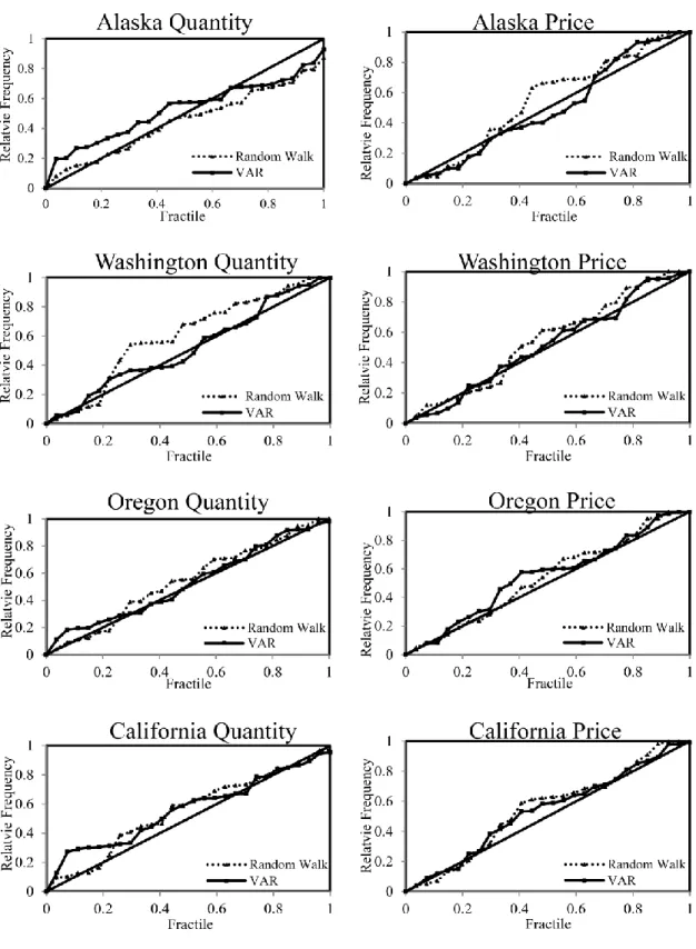
Crab Markets ... 36 Figure III.1. Calibration Functions of the Four State’s Price and Quantity
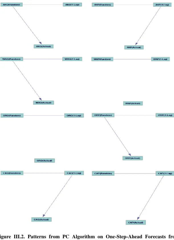
Series, 1986-2012, by 1-lag VAR and Random Walk ... 60 Figure III.2. Patterns from PC Algorithm on One-Step-Ahead Forecasts
from Random Walk (Random) and 1-Lag VAR (1-Lag) and
Actual, 1986-2012. ... 62 Figure IV.1. Actual and Detrended Data on California, Alaska, Washington,
and Oregon Prices and Quantities ... 79 Figure IV.2. Probability and Cumulative Distribution Functions and Empirical
Distribution for Dungeness Crab Detrended Yield Data,
viii
LIST OF TABLES
Page Table II.1. Summary Statistics on Natural Logarithms of Annual Dungeness
Crab Prices (US Cents Per Pound) and Quantities (Pounds), 1950-2002 ... 12 Table II.2. Unit Root Tests on Levels of Log Quantity and Price Series ... 24 Table II.3. Trace Tests of Cointegration among Logarithms of Dungeness
Crab Quantities and Prices ... 26 Table II.4. Descriptive Statistics for the Innovations, 1950-2002 ... 33 Table II.5. Test for Stationary of Levels, Exclusion from the Cointegration
Space, and Weak Exogeneity Test ... 34 Table II.6. Forecasts Error Variance Decomposition of the Eight Series ... 40 Table III.1. RMSE and Goodness of Fit Statistics on VAR and Random Walk
on the Horizon of 1 Step Ahead ... 57 Table III.2. Indicators of Dominance: the 1-lag VAR (1) Versus the Random
Walk (0) for the Goodness-of-Fit Tests and the Causal Graphs ... 63 Table IV.1. Summary Statistics of Annual Dungeness Crab Prices and
Quantities, 1951-2012 ... 81 Table IV.2. Nonstationary Test Results and Trace Tests of Cointegration
among Price and Quantity Variables ... 82 Table IV.3. Goodness-of -Fit Measures and Ranking of Alternative
Distributions ... 89 Table IV.4. Comparisons between the Estimated Data and the Actual Data
from 1951 to 2012 ... 91 Table IV.5. Insurance Premiums for Dungeness Crab and Probabilities of
Paying Indemnities Based on the Yield Coverage Level of 80%, 70%, 60%, and 50% ... 93
1 CHAPTER I INTRODUCTION
Dungeness crab is among the top three most valuable crabs on the West Coast. During the period from 2003 to 2012, the Dungeness crab production ranged from 50 to 89 million pounds, which in the West Coast’s total commercial crab production ranged from 33% to 62%. The crab fishery has an average annual value of approximately $140 million during the same period with more than 43% of the total crab fishery landing values on the West Coast.
Much literature on the Dungeness crab focused on its biology and ecology (e.g., Wild and Tasto 1983; Botsford et al. 1998; Stone and O'Clair 2001; Rasmuson 2013). However, the analyses of the crab prices and production are also important and provide some valuable information for the crab industry. Using economic and statistical models, this dissertation explores price-quantity relationships among the West Coast’s Dungeness crab landing markets and considers an application of prequential analysis to the Dungeness crab prices and quantities. Also, the chance of the Dungeness crab yield losses faced by the fishermen and the crab-yield insurance premiums are estimated. The above topics are included in three main essays (Chapter II-IV), and each essay is stated as following:
The first essay, Chapter II, uses cointegration analysis and directed acyclic graphs to examine the price-quantity dynamics of the western coastal states’ Dungeness crab landing markets including Alaska, Washington, Oregon, and California. Since the Dungeness crab market is special due to its perishable meat and its fishing regulation,
2
the issue of the price-quantity causalities is particularly important in the four landing state markets. If price-quantity relationships exist among the four landing markets, each market is not viewed as a closed economy but an open economy. The directed acyclic graphs contain vertices, edges, and arrowheads to provide an illustration of causal relationships among the four states’ Dungeness crab prices and quantities.
The second essay, Chapter II, conducts prequential analysis to compare the three models (a random walk model and two vector autoregression models) of the four western coastal states’ Dungeness crab landing prices and quantities. As decisions concerning the crab prices and quantities are inherently uncertain and as many if not most decision analyses require expected utility or the entire probability distribution, the prequential analysis is mainly interesting. Pearson’s chi-square test, Kolmogorov-Smirnov test and causal directed acyclic graphs are used to compare the accuracy of the three methods. The model Comparisons not only provide useful information on the Dungeness crab biology and ecology but also has beneficial implications for the Dungeness crab fishery management.
In the third essay (Chapter IV), each state’s fishermen are exposed to the risks of large fluctuations and sharp declines in the Dungeness crab yield but do not have the option to buy a crab-yield insurance policy. Like crop-yield insurance, the crab-yield insurance per pound in cents may be used as a risk management tool to protect the fishermen against the yield and revenue losses. Vector error correction model and goodness-of-fit tests are used to find the parametric probability distributions best describing each western costal state’s crab prices and yields. The probability
3
distributions of the crab yields, those of the crab prices, and Monte Carlo simulation are employed to estimate the insurance premiums of the Dungeness crab yield insurance and the probabilities of the indemnities being paid to the crab fishermen at the coverage levels of 50%, 60%, 70%, and 80%.
4 CHAPTER II
PRICE-QUANTITY DYNAMICS IN THE DUNGENESS CRAB LANDING MARKETS
II.1 Introduction
Dungeness crab is an important commercial crab fishery along the West (Pacific) Coast of the United States (US). During the period from 2003 to 2012, the West Coast’s total commercial crab landing production ranged from 119 to 165 million pounds. The production of Dungeness crab ranged from 50 to 89 million pounds. The commercial Dungeness crab fishery has an average annual value of approximately $140 million during the same period with over 43% of the West Coast’s total crab fishery landing revenues. These statistics show that the Dungeness crab is a high-value product among the West Coast’s crab production1
.
To maintain stock productivity, the commercial Dungeness crab fishery is regulated by the Alaska, Washington, Oregon, and California state legislatures using the “3-S principle” which is based on the crab's sex, season, and size restrictions. Much literature such as Wild and Tasto (1983), Botsford et al. (1998), Stone and O'Clair (2001), and Rasmuson (2013) was concerned with the Dungeness crab biology and ecology. These studies emphasize that Dungeness crab plays a very important role in the West Coast. The analysis of the crab price and quantity is also important and has some beneficial implications for the crab industry. Most of the price-quantity studies ‘described’ the
5
phenomena of some specific regions/states (e.g., Demory 1990; Didier 2002;Dewees et al. 2004; Helliwell 2009). To our knowledge, no empirical research has ‘examined’ the Dungeness crab price and quantity relationships among the four western coastal state landing markets including Alaska, Washington, Oregon, and California.
Economic theory and intuition suggest that a relationship between price and quantity should exist. In practice, the relationships are examined via static models or dynamic causal models. The static methods, a time-invariant system, include the estimation of demand and/or supply functions in equilibrium but have commonly encountered two issues. First, researchers must assume either a quantity-dependent function (i.e., an ordinary function) or a price-dependent function (i.e., an inverse function). Second, the results of estimating the functions may violate the assumptions of economics. That is, the slopes of statistical curves may not equate these to Marshall’s ceteris paribus curves (Moore 1914). With observational data, the existence of omitted variables results in the failure to explain the shifts in demands and supplies whose regularities sometimes look like demand, sometimes like supply, and sometimes neither (Working 1927). The dynamic causal models such as Directed Acyclic Graphs (DAGs) do not have the two problems discussed above but enable us to account for the time dependent effects (i.e. one variable moves the other variables). Mjelde and Bessler (2009) stated that the static models did not present how the relationships respond in the dynamic causal models. In other words, the dynamic but not the static models allow us to examine directly whether the price affects the quantity or is affected by the quantity. The causalities of prices and quantities for some commodities have been described in
6
some studies (e.g., Marshall’s (1920) fish market2, Wang and Bessler’s (2006) meat market3, Helliwell’s (2009) California Dungeness crab market4).
We employ DAGs and vector error correction models (VECM) to identify the causal contemporaneous relationships among the prices and the quantities in the four state Dungeness crab landing markets--Alaska, Washington, Oregon, and California. The principal objectives of the paper are twofold: (i) to understand the degree of the interconnectivity among the four crab landing markets and (ii) to assess whether the quantity-dependent function or the price-dependent function or both or neither exists in the four landing markets. First, the Dungeness crab market is special due to its perishable meat and its fishing regulation. This implies that the issue of the price-quantity causalities is particularly important in the four Dungeness crab landing markets. The important difference between previous studies and our study is that our study tests and examines the price-quantity causalities among the whole landing markets instead of the description of the trade between some specific regions used by some previous studies such as Demory (1990)5 . If the causalities of the prices and quantities exist among the four landing markets, each state landing market would not be viewed as a closed economy but an open economy. The price-quantity interactions in the four state markets
2
Marshall (1920) stated that the quantities caused changes in the prices in a fish market if the stock of fish was taken for granted.
3 Wang and Bessler (2006) showed that retail prices controlled the quantities consumed for poultry and beef products and the quantity of pork controls the pork price.
4
Helliwell (2009) reported that because most of the market crabs were caught within the first two weeks of the fishing season, there was a glut and lower prices.
5 Demory (1990) stated that the California moved the Oregon and Washington price because approximate 70% of Oregon crab was marketed in California. However, Alaska market was excluded in this report.
7
should be considered by each States private and public sectors to make more accurate and complex decisions regarding fishing planning and management. Second, if our results show that price (quantity) is predetermined, the quantity (price)-dependent functions can feature the fundamental market structure; while if the price and the quantity contemporaneously cause each other, the problem of simultaneity would occur and have to be dealt with explicitly (Wang and Bessler 2006).
For the method application and improvement, our contributions include (i) We introduce the new test which combines the concept of Bessler and Wang’s (2012) conjecture model and Kling and Bessler’s (1985) forecast procedures to determine the number of cointegration vectors. The difference between the traditional tests6 and the new tests is that the new tests choose the number of cointegrating rank based the comparison of the forecast performance of the VECM with different cointegration ranks. The VECM model using both the new and the traditional tests will be better suited to estimate and explain the real word than the model just using the traditional tests which do not consider the forecast evaluation. (ii) We compare and apply three DAGs models including greedy equivalence search (GES), Peter and Clark (PC) algorithm, and PC linear non-Gaussian acyclic model (PC-LiNGAM) in the Dungeness crab price-quantity analysis.
The remainder of the paper is organized as follows. A brief discussion of the commercial Dungeness crab industry and its landing data is in the next section, and this
8
is followed by a discussion of the empirical methods. The empirical results are then offered. A summary concludes the paper.
II.2 Industry Overview and Data
The West Coast’s Dungeness crab fishery began commercial fishing since at least 1917 (Miller 1976). The crab dwells in the Pacific Coast from the Pribilof Islands in Alaska to Magdalena Bay in Mexico (Stone and O'Clair 2001), but is not abundant south of Point Conception in California (Pauley et al. 1989). This implies that the commercial harvests of the Dungeness crab come from the four states including Alaska, Washington, Oregon, and California. In addition to meeting the licensing and permitting requirements, the four states’ crab fishermen have to follow the 3-S principle with the “sex-size-season” regulatory system. The 3-S principle asserts that only sexually mature male crabs over the legal size limit are commercially harvested in the fishing seasons every year. The basic commercial crab-fishing regulations have been constant through time but the commercial fishing seasons vary by the management regions. California’s commercial fishing season for Dungeness crab begins the middle of November or the beginning of December and continues through the end of June or the middle of July, and Oregon and Washington have similar fishing-season durations (Hackett et al. 2003). The Dungeness crab has different crabbing seasons throughout the Alaska waters. For example, in southeast Alaska, the season is open in all regions in October and November, open in most areas between the middle of June and of the middle of August, and open in designated regions during the periods from December through the end of
9
February. The season in Kodiak and Alaska Peninsula is open between May and the end of December7. The above information shows that the periods of opening and closing the crab fisheries in Alaska are obviously different from the periods in Washington, Oregon, and California. Moreover, the Dungeness crab stocks have collapsed in some regions of Alaska, possibly due to overfishing, sea otter predation, and adverse climatic changes (Woodby et al. 2005).
Every year the Dungeness crab fishing is banned in the several months when the female crabs are molting and mating or when the male crabs are molting. The extremely low catch in the prohibited months should be found easily in the Dungeness crab’s monthly landing data and might be viewed as a nuisance in statistical analyses. In fact, the complete monthly landing data for the Dungeness crab to date are not available and the missing data problem may cause substantial biases in analyses. To avoid this problem, this study uses the annual landing data.
The data set we analyze consists of 53 annual state-level observations related to the West Coast’s Dungeness crab landing market from 1950 to 2002. It includes the following variables: the commercial quantities of the crab landing in Alaska, Washington, Oregon and California in pounds of round (live) weight (lbs) and their landing prices (US cent/lb). The history series of the four state’s quantities and prices are
7 More information is available at
http://www.adfg.alaska.gov/static/fishing/pdfs/commercial/fishingseasons_cf.pdf. Cited 30 November, 2013.
10
obtained from the NOAA’s National Marine Fisheries Service (NOAA Fisheries). Data was also collected from 2003 through 2012 for an out-of-sample forecast evaluation.
The original data are transformed to the natural logarithm of the values of the variables to improve the normality of variables, and plots of the natural logarithm of each price and quantity series between 1950 and 2012 are given in figure II.1. Notice that for each market, landing price series appear to have trends over time and to be mean non-stationary processes. For the four landing quantity series, whether their processes are non-stationary is less obvious. Each states commercial Dungeness crab fishery has exhibited periods of high and low landings. Especially, between northern California and Washington, the crab fishery synchronously undergoes cyclic catch fluctuations in abundance (Botsford et al. 1998). The cycles are caused by: (i) predator-prey systems with both salmon and human as predictors, (ii) exogenous environmental forces such as ocean temperature, surface winds, alongshore flow, and sea level, (iii) density-dependent (biological) mechanisms containing density-dependent fecundity, an egg-predator worm and cannibalism (Botsford et al. 1998).
Summary statistics of the natural logarithms of the within-sample data from 1950 through 2002 are presented in table II.1. During the period, Washington had highest average Dungeness crab landings, followed by Oregon, California and Alaska. California’s crab quantities appear to be most volatile among the four states’ landings, as measured by Coefficient of variation representing the degree of dispersion in each series. For the four states’ crab prices, California had the highest average, followed by Oregon, Washington and Alaska. It is noteworthy that California’s crab had the highest average
11
price but the lowest volatility in its prices. However, the crab prices in Alaska were the lowest in average but fluctuated most dramatically.
Figure II.1. Time Series Plots of Natural Logarithms of Dungeness Crab Quantities and Prices, 1950-2012
12
Table II.1. Summary Statistics on Natural Logarithms of Annual Dungeness Crab Prices and Quantities, 1950-2002
State Mean Standard Coefficient Minimum Maximum
Deviation Variation Quantity (lbs) Alaska 15.52 0.67 0.18 13.22 16.57 Washington 16.07 0.53 0.14 15.19 17.13 Oregon 15.92 0.49 0.12 14.63 16.81 California 15.88 0.75 0.19 13.44 17.33 Price (cents/lb) Alaska 3.61 1.19 0.33 1.61 5.41 Washington 3.88 1.07 0.28 2.09 5.37 Oregon 3.90 1.08 0.28 2.08 5.36 California 4.00 1.02 0.26 2.15 5.54
II.3 Models and Methodologies
II.3.1 Vector Error Correction Model (VECM)
Empirical economics does not suggest a prior structure for the causality among the four-state Dungeness crab’s landing prices and quantities. Therefore, if some series in the evaluated price and quantity data are non-stationary and cointegrated, the error correction framework is viewed as the basic and useful tool for analyzing the above dynamic relationship. The VECM framework is well-developed by Engle and Granger (1987), Hansen and Juselius (1995), Jonathan (2006), Juselius (2006):
II.(1) ∆𝑌𝑡 = Π𝑌𝑡−1+ ∑𝑘−1𝑖=1 Γ𝑖Δ𝑌𝑡−𝑖+ 𝜇 + 𝑒𝑡 (𝑡 = 1, … , 𝑇)
where ∆Yt is the first differences (Yt−Yt-1), Yt is a (𝑚 × 1) vector of the four-state price
and quantity variables at the time t (m=8 in this study), Π is a (8 × 8) matrix of coefficients relating the lag of the variables in levels to current changes in variables, Γi is
13
a (8 × 8) matrix of coefficients relating the i-period lagged variable changes to current changes in variables, μ is a (8 × 1) vector of constant, and et is a (8 × 1) vector of a
number N of independent, identically distributed (i.i.d) innovations (i.e., error terms). Π has reduced rank and can be represented as αβʹ, where α and β are 8 × 𝑟matrices of full rank, and r, a positive number less than or equal to the number of series, is defined as the rank of Π (i.e., the number of cointegration relationships).
Various procedures have been widely used to determine cointegrating rank such as Johansen’s trace test (Juselius 2006), Schwarz information criterion (Phillips 1996; Wang and Bessler 2005) and Hannan and Quinn (HQ, 1997) information criterion and so on. The trace test requires two steps: the trace test for the cointegration vector being identified posterior to the selection of the lag length in a vector autoregression (VAR). While, by minimizing the information criteria, the researchers are allowed to jointly determine the lag length and the cointegrating rank over a pool model with various lag lengths and cointegrating ranks (Wang and Bessler 2005). In fact, the VECM has been used in practice for extrapolating past economic behavior into the future (i.e., forecasting). Unfortunately, the above tests and information criteria used to determine the number of cointegrating vectors is not mainly based on examination of the out-of-sample forecasting performance and thus likely yield problems with forecasting accuracy. The VECM models with various lag lengths or/and various cointegrating ranks may have different predictive performances. We introduce and apply the two methods considering forecast performance to select the number of cointegrating vectors: the forecast procedures (Kling and Bessler 1985) and the conjecture model (Bessler and
14
Wang 2012). In order to best describes and fits the Dungeness crab data using the VECM model, the results from the two forecasting models and those from the three frequently used methods are all compared to determine the number of cointegrating ranks.
Kling and Bessler’s 1985 forecast procedures require two subsamples of data (i.e., within-sample and out-of-sample data) and then compares the out-of-sample forecast results for the variations (e.g., the VECM models with different ranks) on the basis of root mean square (RMS) error and ln determinant. In this study, the forecasts for each series with one through eight cointegrating ranks are examined in accordance with RMS; and as an overall measure for the VECM model with each rank, the ln determinant of the covariance matrix of forecast errors is evaluated. The second procedure of determining the rank of Π used in this study is the conjecture model as defined by Bessler and Wang (2012):
Definition: “Scientists implicitly seek a model, theory, or explanation whose forecasts d-separate predictions that are derived from inferior models, theories, or explanations and Actual realizations of the world” (Bessler and Wang 2012).
The conjecture model assumes that the Actual realization come in real time after any forecasts, so the information flow flows from the Actual never come back to any forecast. Here, several sets of forecasts on each series emanate from the VECM models with the same data but with different ranks of Π. Then, we test the hypotheses that the information links among data forecasts from the model with different cointegrating ranks and the Actual realization of the variable of interest. D-separation (described later) offers
15
a succinct notion to illustrate that one set of forecasts dominates over the other sets on each series, and the dominating set whose rank is selected as the candidate for the number of the cointegrating vectors. Actually, the series may have different candidates so that the most frequent number among the candidates of all the series is the best choice for the number of cointegrating ranks used in the VECM model.
Through the parameters in equation II.(1), the VECM can be composed of three-part information: the long-run, short-run and contemporaneous structure. The long-run structure can be identified through testing hypotheses on the parameter β, while hypotheses on the parameters α and Γi are related to the short-run structure (Hansen and
Juselius 1995; Juselius 2006). Furthermore, the contemporaneous structure can be summarized through structural analysis of et (Swanson and Granger 1997). We examine
tests of hypotheses on the cointegration space including test for exclusion and test for weak exogeneity.
The test of exclusion provides useful information on whether each price and quantity series enters all of the identified long-run relationships. The null hypothesis is that each series is not in the cointegration space or alternatively stated, βij = 0, for i =
1,…,8 and j =1,…,r (Hansen and Juselius 1995). Under the null, the test statistic is asymptotically distributed as chi-square with r degrees of freedom. The test of weak exogeneity examines whether each series does not react to the long-run disequilibrium. Under the null hypothesis that αij = 0, for i = 1,…,8 and j =1,…,r, the test statistic is
distributed as chi-square with degree of freedom equal to the number of the rank of Π (Hansen and Juselius 1995).
16
It is difficult to make sense of the coefficients of the VECM (Sims 1980). Accordingly, innovation accounting technique may be the way to describe the dynamic structure and the interactions among the time series (Sims 1980; Lütkepohl and Reimers 1992; Swanson and Granger 1997). Here, the estimated VECM is algebraically converted to a levels VAR. The innovation accounting based on the equivalent levels VAR is then generated to summarize the dynamic interaction among the price and quantity series. The forecast error variance decompositions over a variety of horizons are shown in this study.
Swanson and Granger (1997), Spirtes, Glymour and Scheines (2000), Hoover (2005), and Hyvärinen et al. (2010) suggest that the information on the causal relationships among innovations in contemporaneous time can be examined based on the information of the error terms in the autoregressive models. The DAGs are used in this paper to obtain data-determined evidence on the contemporaneous causal ordering, under the assumption that the information set is causally sufficient (Spirtes, Glymour, and Scheines 2000; Shimizu et al. 2006; Pearl 2000; Hoyer et al. 2008). A Bernanke ordering dealing with contemporaneous innovation is based on the discovered structure from the DAGs (Swanson and Granger 1997).
II.3.2 Directed Acyclic Graphs (DAGs)
DAGs contain vertices, edges, and arrowheads but no self-loops and no directed cycles to provide an illustration of causal relationships among a set of variables (Pearl 2000). Recently, under different assumptions of the data (i.e. the statistical properties of
17
the data) and in different ways, several methods such as the linear-Gaussian approach8 (Spirtes, Glymour, and Scheines 2000; Pearl 2000), linear-non-Gaussian approach (Shimizu et al. 2006), and combination of the two above approaches (Hoyer et al. 2008) have been developed to discover the acyclic causal structure of the observational data. A key difference among these three approaches is the assumption of Gaussian/ non-Gaussian/ partial Gaussian innovations. Causal diagrams for empirical studies may be biased and unreliable when the innovations are departing from the assumptions of the used approaches. The study diagnoses the distribution of innovations and subsequently selects and compares the well-suited algorithms of DAGs to understand the price-quantity relationships of the four Dungeness crab landing markets. The followings are the basic concepts, assumptions, applications of the three approaches:
II.3.3 Linear-Gaussian Acyclic Approach
Under the assumption of Gaussianity of disturbance variables, several authors (Spirtes, Glymour, and Scheines 2000; Pearl 2000) use DAGs for the purpose of discovering conditional independence relations in a probability distribution. That is, an assumption of Gaussianity which means an unskewed distribution (i.e., a symmetric distribution) allows that conditional correlation can be completely estimated just from the covariate matrix (i.e., second-order statistics) but not from higher-order moment structure. This line of research implies that the conditional independence cannot separate between independence-equivalent models. Mathematically, the Gaussian DAG models
18
represent conditional independence as implied by the recursive production decomposition:
II.(2) 𝑃𝑟(𝑣1, 𝑣2, … , 𝑣𝑛 ) = ∏𝑛𝑖=1Pr (𝑣𝑖|𝑝𝑎𝑖),
Where Pr denotes the probability of variables (i.e., vertices) v1, v2,…, vn, pai is the
realization of some subset of the variables that precede vi in order (i=1,2,…,n), and the
symbol Π is the product (multiplication) operator. Pearl (2000) proposes d-separation (i.e., direct-separation viewed as a graphical characterization of conditional independence shown in equation II.(2). If the information between two vertices (for example, variables X and Y) is block, the information is said to be d-separation from the one variable (X) to the other variable (Y). That is, the d-separation occurs if (i) a fork chain X ← Z → Y or a causal chain X → Z → Y exists such that the middle variables Z is in the information; or (ii) an inverted fork X → Z ← Y exists such that the middle variable (a collider) Z or any of its descendent is not in the information.
If we formulate a DAG in which the variables (v1, v2,…, vn) corresponding to pai are
illustrated as the parents (directed cause) of vi, then the independencies applied by
equation II.(2) can be read off the graph using the d-separation criterion. Geiger, Verma and Pearl (1990) revealed that there is a one-to-one correspondence between the set of conditional independencies, 𝑋 ⊥ 𝑌|𝑍, implied by equation II.(2) and the set of triples (X, Y, Z) that satisfy the d-separation criterion in graph G. Specifically, suppose that G is a DAG with variable set V in which X and Y as well as Z exist, then G linear implied the zero correlation between X and Y conditional on Z if and only if X and Y are d-separation given Z.
19
Several alternative algorithms learning the DAGs from the Gaussian distributed data have been studied for decades, but two alternative algorithms based on either conditional independence constraints or Bayesian scoring criterion are often used and compared with each other (e.g., Wang and Bessler 2006; Kwon and Bessler 2011). That is, in both of the frameworks that the algorithms are used to obtain the DAGs from the variance/covariance matrix with VECM innovations under Markov condition (i.e., acyclic and causal sufficiency condition), and faithfulness assumptions9, the PC algorithm (Spirtes, Glymour, and Scheines 2000) relies on constraint-based test while the GES algorithm (Chickering 2002) search the space of models using a score.
The PC algorithm starts systematically from a completely connected undirected graph G on the set of variables to be determined. Edges between variables are removed sequentially based on zero unconditional correlation and partial correlation (conditional correlation) at some pre-specified significance level of normal distribution. The conditioning variable(s) on the removed lines between two variables is called the sepset,
as defined in Bessler and Akleman (1998), of the variables whose line has been removed
(for vanishing zero-order conditioning information the sepset is an empty set). For a simplified example of triples X−Y−Z, X−Y−Z can be directed as an inverted fork X→Z←Y if Z is not in the sepset of X and Y (that is, the zero unconditional correlation between X and Y). If the correlation between X and Y conditional on Z is zero, the
9 According to Kwon and Bessler (2011), the causal Markov condition which consists of acyclic and causal sufficiency (i.e, mutual independent error terms or the assumption of no latent variables) is assumed in most empirical studies, although using the condition can be problematic. The faithfulness assumption is that all the (un)conditional probabilistic structures are stable (i.e. faithful or a DAG-isomorphism) with respect to changes in their numerical value.
20
underlying model may have been a fork chain X ← Z → Y or a causal chain X → Z → Y. Hence, the edge between X, Y and Z would not be directed so that the undirected edges X−Z−Y would be left under the PC algorithm.
At small sample size, the PC algorithm may erroneously add or remove edges and direct edges at the traditionally applied significance level (e.g., 0.1 or 0.05). Monte Carlo studies with small sizes has been well discussed in Spirtes, Glymour, and Scheines (2000, pp. 116): “In order for the model to converge to the correct decisions with probability 1, the significance level used in making decisions should decrease as the sample sizes increase, and the use of higher significance levels (e.g., 0.2 at the sample sizes less than 100, and 0.1 at sample sizes between 100 and 300) may improve performance at small sizes.” The PC algorithm would be applied at the significance level of 0.2 in this study due to our sample sizes less than 100.
The GES algorithm is a two-phase algorithm that searches over alternative DAGs using the Bayesian information criterion as a measure of scoring goodness fit. The algorithm begins with a DAG representation with no edges. A DAG with no edges implies independence among all variables. Edges are added and/or edge directions reversed one at a time in a systematic search across classes of equivalent DAGs if the Bayesian posterior score is improved. The first stage ends when a local maximum of Bayesian score is found such that no further edge additions or reversal improves the score. From this final first stage DAG, the second stage commences to delete edges and reverse directions, if such actions result in improvement in the Bayesian posterior score. The algorithms terminates if no further deletions or reversals improve the score.
21
II.3.4 Linear-Non-Gaussian Acyclic Model (LiNGAM)
Even though linear-non-Gaussian acyclic Model (LiNGAM) is not employed in this study, it is an important part to form the PC-LiNGAM algorithm. The brief introduction to LiNGAM is interpreted as follows.
When the Markov condition and the assumption of non-Gaussian innovations are both valid10, the LiNGAM allows the complete causal structure of the non-experimental data to be determined without any prior knowledge of network structure (such as a causal ordering of the variables). Here, the non-Gaussian structure may provide more information than the covariance structure which is the only source of information in the linear-Gaussian acyclic approach. The first algorithm for LiNGAM, ICA-LiNGAM proposed in Shimizu et al. (2006), is closely related to independent component analysis (ICA) (Hyvärinen, Karhunen, and Oja 2004) and is applicable to purely non-Gaussian data. The key to the solution of the ICA-LiNGAM algorithm is to realize that the observed variables are linear functions of the mutually independent and non-Gaussian innovations. Details on the process of the ICA-LiNGAM model identification are given in Shimizu et al. (2006, pp. 2006-2008). It is worthy noting that the ICA-LiNGAM algorithm is inapplicable to data which is partially Gaussian (Hoyer et al. 2008) or which has more than one Gaussian distributed series (Hyvärinen et al. 2010).
10 The algorithm with the three assumptions is called LiNGAM: (1) the recursive generating process, (2) the linear data generating process, (3) mutually-independent and non-Gaussian innovations with arbitrary (non-zero) variances. Note that the recursive generating process means the graphic representation by DAGs; the independence of the innovations implies non-existence of unobserved confounders or the causally sufficiency. Also note that LiNGAM does not require the faithfulness (or stability) of generating model. See Shimizu et al. (2006, pp. 2004-2005) for details on the LiNGAM assumptions and properties.
22
II.3.5 Combination of the Gaussian and Non-Gaussian Approaches
PC-LiNGAM algorithm (Hoyer et al. 2008) combines the strengths of the approaches purely based on conditional independence and those of the ICA-based methods. An important goal in the algorithm is to show the distribution-equivalence patterns that identify DAGs in mixed Gaussian/ non-Gaussian models11under the Markov condition and the faithfulness assumption. The PC-LiNGAM algorithm consists of three stages: First, the PC algorithm is used to obtain the d-separation equivalence class. Second, all DAGs in the first-stage estimated equivalence class are scored using the ICA objective function12, and then the highest-scoring DAG (i.e., the DAG with least dependent estimated innovations) is selected. The third step identifies the correct distribution-equivalent class: construct equivalence-class based on the estimated DAG and the results of the tests for Gaussianity for the estimated innovations.
The four algorithms discussed here including PC, GES, ICA-LiNGAM, and PC-LiNGAM algorithms are available under the Tetrad project at Carnegie Mellon University. We conduct the four algorithms, generate several DAGs, and then select the
11 The PC-LiNGAM algorithm does not require the Gaussian nor non-Gaussian distributed innovations. 12
The ICA objective function U , as a measure of the non-Gaussianity of a random variables, is shown in Hoyer et al. (2012) :
𝑈 = ∑ (𝐸 {|𝑒𝑖 𝑖| − √2 𝜋⁄ })2 ,
where ei are the mutually-independence innovations with arbitrary densities. The function can be shown to provide a consistent estimator for searching the independent components under the weak conditions. However, it has two limitations: First, the disregarded sampling effects may lead that distribution-equivalent models obtain exactly the same value of U. However, the practical case of a finite sample is not the case because the correct distribution-equivalent class is identified in the final stages of the PC-LiNGAM algorithm. Second, the objective function may mislead due to the linear correlation among the estimated innovations.
23
best-described causal structure among these DAGs to represent the price-quantity relationships of the four Dungeness crab markets.
II.4 Empirical Results
All estimations are carried out in terms of the natural logarithms of the price and quantity series. The first 53 observations (within-sample data) are first considered to the time series properties of the VECM model, while about 16% of the entire data is reserved so they can be used for out-of-sample forecasts to determine the number of cointegrating vectors.
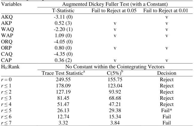
In order to determine whether the VECM model is appropriate for the Dungeness crab landing price and quantity series, the two unit root tests on the levels of the within-sample data are applied: Phillips and Perron (1988) and Augmented Dickey-Fuller (ADF,1981) tests. The Bayesian information criterion (BIC) is conducted as a selection criterion to select the appropriate lag lengths contained in the ADF test with a maximum of four lags. Results of the both tests are the same shown in table II.2. Each state’s price series is non-stationary at the 5% significance level. Moreover, the null hypotheses of non-stationarity for the Alaska, Oregon and California quantity series are rejected, but the tests fail to reject the null hypothesis for the Washington quantities. Although the Washington quantity series is non-stationary at the 5% significance level, the t-statistics
24
(-2.67) appears to be close to the critical value of -2.9213. The following phenomena may contribute to these stationary quantity series. The Dungeness crab catch records along the Pacific Coast vary in a cyclic pattern (Botsford et al. 1998). The crab abundance peaks in around 10-year cycles (Dewees et al. 2004). Nevertheless, the two unit root tests show at least two series in the evaluated data are non-stationary, thus a multivariate cointegration model is appropriate (Hansen and Juselius 1995).
Table II.2. Unit Root Tests on Levels of Log Quantity and Price Series
Series Philips-Perron Test Augmented
Dickey-Fuller Test
Log Alaska Quantity (LAKQ) -3.21 -3.15 (0)
Log Alaska Price (LAKP) -1.23 * -1.21 (0) *
Log Washington Quantity (LWAQ) -2.72 * -2.67 (0) *
Log Washington Price (LWAP) -0.77 * -0.75 (0) *
Log Oregon Quantity (LORQ) -4.30 -4.22 (0)
Log Oregon Price (LORP) -0.96 * -0.94 (0) *
Log California Quantity (LCAQ) -3.44 -5.19 (2)
Log California Price (LCAP) -1.10 * -1.08 (0) *
Note: Numbers in parentheses are the lags included in ADF test to reach a minimum BIC. “*” means the series is non-stationary at 0.05.
13 The Washington quantity series is not non-stationary at the 10% significance level since the t-statistics is less than the critical level of -2.60.
25
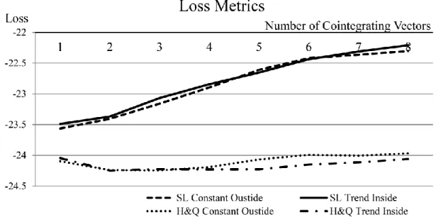
The appropriate lag length (k) in the VECM model of the equation II.(1) is one, chosen on the basis of the BIC with a maximum of four lags. Previous studies have determined the number of cointegrating vectors using the trace test, the Schwarz information criterion, and the HQ loss measures. All the three tests for determining the number of cointegrating ranks for both14 no constant within (a constant outside) and linear trends within the cointegrating vectors are conducted in this study with the CATS in RATS program. It is noticeable that the CATS calculates the rank test statistics for the VECM model at each level of cointegration but excludes the statistics for zero rank (no cointegrating vector). Following the sequential testing procedure of the trace test (Hansen and Juselius 1995), table II.3 is read from left to right and from the top to bottom. The first failure to reject the null hypothesis in this sequence is less or equal to two in the case of a constant outside the cointegrating space. Figure II.2 shows plots of both the Schwarz and HQ loss measures at each level of cointegration for the zero constant or the linear trends inside the cointegrating vectors. Generally, the Schwarz measure fits the same or lower order than HQ measure. The Schwarz measures are minimized at one rank with the constant outside the cointegration space; while the HQ measures reach minimum at two ranks with the trend inside the cointegration space. Unfortunately, the three rank-based tests determine the three combinations (different
14 The CATS are used to conduct the four VECM models with the different assumptions about the constant term and linear trends (Hansen and Juselius, 1995): (1) the model with neither the constant nor trends; (2) the model restricting the constant to the cointegration space; (3) the model having a constant outside the cointegration space; (4) the model with the linear trends inside the cointegration space. The VECM model without any deterministic components should be used carefully because at least a constant is very likely in the cointegration space. The VECM model with a constant within the cointegration space does not fit the Dungeness crab data well. Hence, we consider the last two models.
26
ranks with different components inside the cointegration relations). In many empirical studies, the VECM model with the trends inside the cointegrating vectors is rarely applied. Besides, the results of both the trace test and the Schwarz measure support no constant in the cointegraiton space, which would be imposed on the model of the Dungeness crab’s landing markets.
Table II.3. Trace Tests of Cointegration among Logarithms of Dungeness Crab Quantities and Prices
H0:Rank
No Constant within the
Cointegrating Vectors
Linear Trend within the Cointegrating Vectors Tracea C(5%)b Decision Tracea C(5%)b Decision
r = 0 189.47 155.75 Reject 216.23 182.45 Reject r ≤ 1 128.04 123.04 Reject 154.69 146.75 Reject r ≤ 2 84.85 93.92 Fail* 105.63 114.96 Fail r ≤ 3 54.25 68.68 Fail 73.82 86.96 Fail r ≤ 4 32.35 47.21 Fail 46.09 62.61 Fail r ≤ 5 19.60 29.38 Fail 24.27 42.20 Fail r ≤ 6 9.77 15.34 Fail 11.83 25.47 Fail r ≤ 7 0.75 3.84 Fail 2.65 12.39 Fail
a Trace refers to the trace statistic considering the null hypothesis that the rank of Π is less than or equal to r.
b C(5%) refers to the critical values at the 5 percent level. If the trace statistics exceeds its critical value, the null hypothesis is rejected.
27
Figure II.2. SL and HQ Statistics for Different Numbers of Cointegrating Rank in VECM Model with the Constant Outside and the Trends inside the Cointegration Space
Unlike the three tests without consideration of the out-of-sample forecast, the RMS error, the ln determinant, and the conjecture model are also used to select the number of cointegrating vectors. The two-step procedure is used. First, the forecast statistics of the RMS error and the ln determinant are calculated (in RATS). Figure II.3 ranks the VECM model with different numbers of cointegrating vectors according to ln determinant and RMS error at the one-step ahead. The RMS errors are useful for evaluating the forecast performance of the individual price/quantity series with zero through eight cointegrating vectors. For the Alaska price and quantity series, one cointegrating vector performs best. Zero cointegrating vectors appear to be best suited in the Washington price and quantity,
28
and the Oregon and California price equations respectively. Both the Oregon and the California quantity series rank the five cointegrating vectors first. One way to obtain a rough determination of the number of cointegrating vectors in the overall VECM model (not in the individual equations), is to average the best-performing numbers of cointegrating vectors across the eight series. The number is 1.5 and this implies that one or two cointegrating vectors may provide the best forecasts, providing the best overall performance of the model. With respect to the ln determinant measures, zero cointegrating vector performs best, followed by one cointegrating vector. By combining both the RMS and ln determinant results, the VECM model with zero, one, or two cointegrating vectors (the three sets) may perform better than the models with the other numbers.
29
Figure II.3. RMS Errors of Logarithms of Dungeness Crab Quantities and Prices and Log Determinant
30
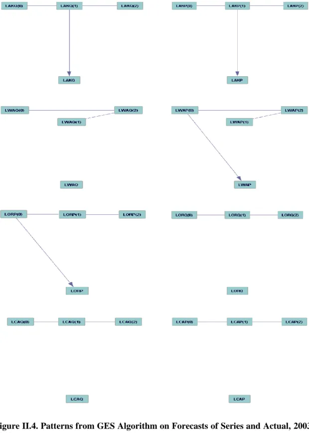
The second step is to search among the three sets using the conjecture model to find the best. That is, the GES algorithm15 assesses the “causal” relationships among these three sets of cointegrating vectors for generating price/quantity forecasts and Actual prices/quantities (the out-of-sample data) subject to the restriction that the Actual is unable to affect the forecasts. The patterns for one-step ahead are summarized in figure II.4. The forecasts from the one cointegrating vector directly arrow toward the Actual level for the Alaska price and quantity respectively, While the forecasts from the zero cointegrating vector is of high quality in the Washington and Oregon price series. Obviously, the forecasts from the zero or one cointegrating vector are the most common direct cause of the Actual data, and the probability of choosing both by the price/quantity series is 50% respectively.
If the results from the three forecasting tests and the three traditional ranked-base ones are all considered, half of these tests (the Schwarz measures, ln determinants measure, and conjecture model) select the one cointegrating rank. Hence, one may expect to see this one cointegrating vector with the constant outside the cointegration space among the four states’ Dungeness crab price and quantity series.
15
GES algorithm and PC algorithm, as provided in the TETRAD umbrella, allow researchers to apply Knowledge tiers that prevent the Actual from cause the forecasts. Since the GES algorithm provides more information on the causal relationships than the PC algorithm here, the patterns of the GES algorithm are shown in this study.
31
Figure II.4. Patterns from GES Algorithm on Forecasts of Series and Actual, 2003-2012
32
Before discovering the price-quantity causal structure of the Dungeness crab, we need to understand the statistical properties16 of the innovations and tests for stationary, exclusion and weak exogeneity. For the case with the single cointegrating rank, Lagrangian Multiplier tests (Hansen and Juselius 1995) on first and fourth order autocorrelation cannot be rejected at usual levels of significance. In facts, we reject first order autocorrelation at a p-value of 0.13 and four order autocorrelation at a p-value of 0.43. The four moments of the innovations of each series including mean, standard deviation, skeweness and kurtosis are shown in table II.4. Based on the skewness and kurtosis of multivariate innovations, Doornik-Hansen test (2008) examines the null hypothesis of the multivariate normal innovations. The innovations with one cointegrating vector (the p-value of 0.041) is normal distributed at the 1% significance level but is not at the 10% or 5% significance level. The choice of the different significance levels (α=1%, 5%, or 10%) decides either the normality of the innovations or the non-normality of the innovations. The univariate normality tests for the eight series in table II.4 show that more than one of the innovations are normal at the 1%, 5%, or 10% levels, suggesting that the LiNGAM algorithm is unable to employed in this study. To avoid losing information from this type of the innovations, the PC, GES, and PCLiNGAM algorithms are all used to search the causal relationship among the four Dungeness crab landing markets.
16
The univariate statistics for the estimated residuals of each equation obtained by CATS in RATS differ from those obtained by RATS’ STATISTICS instruction (Jonathan, 2006). Moreover, CATS in RATS does not provide the statistical measures for the VECM model with zero rank. For these reasons, the statistical properties of the model are executed by RATS.
33
Table II.4. Descriptive Statistics for the Innovations, 1950-2002
Variables Mean Standard
Deviation
Skewnessa Kurtosisb Normalityc (p-value) (p-value) (p-value)
LAKQ 0.00 0.54 0.34 1.43 6.23 (0.33) (0.05) (0.04) LAKP -0.00 0.28 0.27 1.24 5.29 (0.43) (0.09) (0.07) LWAQ -0.00 0.38 0.10 0.33 1.20 (0.78) (0.65) (0.55) LWAP -0.00 0.20 0.46 0.46 2.27 (0.19) (0.52) (0.32) LORQ -0.00 0.47 -0.11 0.05 0.44 (0.75) (0.95) (0.80) LORP 0.00 0.20 -0.16 -0.56 0.73 (0.65) (0.44) (0.70) LCAQ 0.00 0.63 -0.34 1.25 5.21 (0.33) (0.09) (0.07) LCAP 0.00 0.24 0.13 0.18 0.75 (0.71) (0.81) (0.69)
Note: See table II.2 for the definition of variables. The four moments and normality test of the innovations of each series from the VECM model are estimated using RATS.
a The null hypothesis of skewness tests states that skweness of each series is zero. b Kurtosis tests are related to the null hypothesis of kurtosis of each series being zero. c
Doornik–Hansen univariate normality tests consider the null hypothesis that each series has normal distribution. The results show that Alaska price and Quantity and California quantity are not normally distributed at the 0.1 level while the other series are normal.
Given this single cointegrating vector, some exploratory tests on the long-run interdependence among these eight price/quantity series are further conducted. First, we explore the possibility that a long-run relationship (cointegrating vector) arises because one or more of the series is itself stationary, especially since the ADF test suggests that the three quantity series are potentially stationary (Alaska, Oregon, and California Quantity see table II.2). As presented in table II.5, the null hypothesis that each series is itself stationary in the cointegration space is clearly rejected at very low p-values. The
34
test results suggest that the one cointegrating vector arises from a linear combination of the eight individual series.
Table II.5. Test for Stationary of Levels, Exclusion from the Cointegration Space, and Weak Exogeneity Test
Series Test
Stationarya, df=7 Exclusionb, df=1 Weak Exogeneityc, df=1
LAKQ 49.44 0.08 1.10 LAKP 58.98 6.02 0.02 LWAQ 53.13 13.70 2.59 LWAP 59.74 0.01 1.70 LORQ 41.50 8.31 4.28 LORP 59.49 17.97 8.17 LCAQ 48.45 0.85 3.12 LCAP 59.19 11.76 0.94 Critical (5%) 14.07 3.84 3.84
aStationarity tests are on the null hypothesis that the series listed in the column heading is one of the one stationary relationships found in figure II.4.
b
Exclusion tests are related to the null hypothesis that the series is not in the cointegration space.
cWeak exogeneity tests consider if the series does not respond to the perturbations in the cointegration space.
Exclusion and weak exogeneity test results are also shown in table II.5. In the exclusion test, we consider the possibility that a particular series of the eight series is not in the cointegrating space. Except for the Alaska and California quantities and the Washington price, the null hypotheses associated with the other five series are rejected at the 5% significance level, suggesting they are part of the long-run relationship. The tests of weak exogeneity explore the possibility that some series do not respond to
35
perturbations in the long-run equilibrium (cointegrating vector). From the table we do not reject the null hypotheses for the other six series, except for the Oregon price and quantity. This suggests that the Oregon price and quantity are the only two series to make adjustment toward the estimated long-run equilibrium when the perturbations happen.
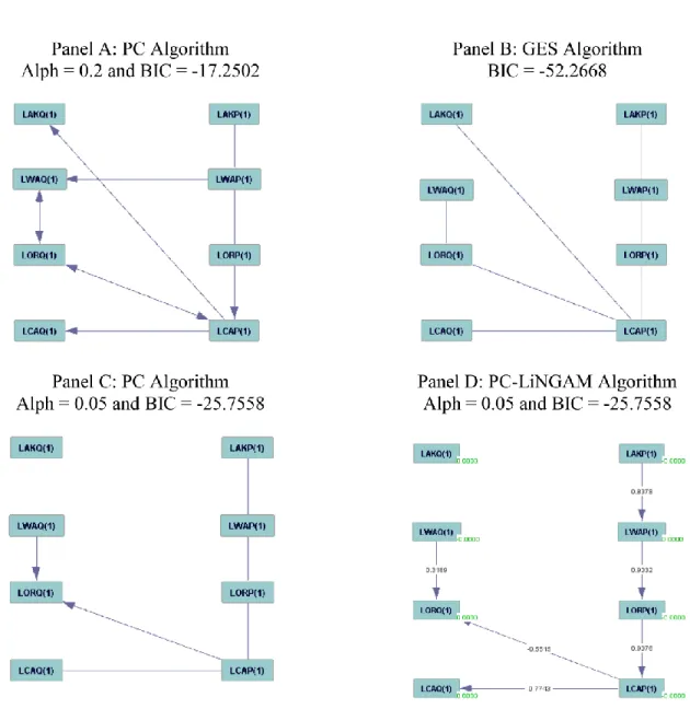
Applied to the innovations, the contemporaneous causal relationships from the GES, PC, and PC-LiNGAM algorithms are shown in figure II.5. The results from the PC algorithm at the significance level of 0.2 (figure II.5A) indicate that the double-headed arrow exists between the Washington and Oregon Quantities. Such an arrow is the result of a partial failure of the PC algorithm under violation of its assumptions, and then the 0.05 significance level is used to replace the 0.2 level. Among these DAGs in figure II.5, the DAG using the GES algorithm has the lowest BIC score, followed by the PC-LiNGAM or PC algorithms using the 0.2 significance level. It seems that the GES algorithm performs best, but represents the undirected relationships (e.g., the undirected edges) among the four states’ Dungeness crab prices and quantities (figure II.5B). Such undirected edges also exist in the DAG with the PC algorithm (figure II.5C). Clearly, the Alaska price, the Washington price, the Oregon price, the California price, and the California quantity are linked but the causality is unknown. To determine the causal relationships among the linked but undirected series in figure II.5C, the PC-LiNGAM algorithm is employed and a causal chain from the Alaska price to the California quantity through the Washington, Oregon, and California prices is determined (figure
36
II.5D). Hence, the figure II.5D is the finalized DAG depicting the contemporaneous relationships among the four states’ prices and quantities.
Figure II.5. Patterns of Causal Flows among the Four States’ Dungeness Crab Markets Note: Pattern finally determined using PC-LiNGAM algorithm in Tetrad V (2014). Numbers in parentheses are the number of cointegrating vectors.
37
More interestingly, some of the results obtained from the PC-LiNGAM algorithm are consistent with the literature on the Dungeness crab movement patterns and the actual findings. First, considering the relationship of the four state’s Dungeness crab landing quantities (especially for sexually mature male), the figure II.5D clearly shows there are no directed edges between the states which are not adjacent to each other. That is, from an ecological perspective, the results suggest that the adult male Dungeness crab in the one state is unable to move across the neighboring states to the other state (i.e., the Oregon (Alaska) crab cannot migrate to Alaska (Oregon)). Combination of the information on the length of each state’s coastline and the literature on the Dungeness crab movement (i.e., Stone and O'Clair 2001) implies that the crab cannot move to the unadjacent states. Second, the Alaska quantity is not linked to the other prices and quantities. This may result from the Alaska Dungeness crab stock collapse17 and different crabbing seasons throughout Alaska.
Figure II.5D clearly shows that the four states’ Dungeness crab prices are strong connected in contemporaneous time, and are determined by the PC-LiNGAM as a causal chain from the Alaska price to the California price through the Washington and the Oregon prices. Here, the Alaska price and the Washington quantity are both the information initiator in the Dungeness crab markets, while the other three states’ prices
17 The fisheries for Dungeness crab have historically occurred throughout the Alaska coast, but several stocks in the Alaska such as Prince William Sound, Copper River delta, and Kachemak Bay area have collapsed. The possible causes of these collapses include overfishing, sea otter predation, and adverse climatic changes. The Dungeness crab fishery in Yakutat has been close since 2001 due to the stock collapse in 2000. In contrast, Southeast Alaska and the Kodiak area remain open to support mainly small boat fisheries with harvests fluctuating. See Woodby et al. (2005) for the Alaskan Dungeness crab fishery.
38
(excluding the Alaska price) and the California and Oregon quantities receive information. The tri-state Dungeness crab committee18 including Washington, Oregon, California was formed in 1998 to devote the three states’ management of Dungeness crab. This suggests that the price and quantity relationships among the three states’ markets should exist. Such relationships shown in figure II.5D are described below.
The Washington quantity actively generates information and passes it to the Oregon quantity within a year. The Oregon and California quantities are information “sinks.” That is, the Oregon quantity receives information from both the Washington quantity and the causal chain of the four states’ prices, but does not pass it on other prices and quantities. The California quantity receives information from the causal chain of the prices through the California price. The information flow of the prices (the causal chain) may be blocked on its path to the Oregon and California quantities by the California price. The fact that the California price causes its own quantity suggests that the quantity-dependent function exists in the California Dungeness crab market.
Based on the estimated results of the equation II.(1) together with the causal structure in figure II.5D, the forecast error variance decomposition (table II.6) measures the dynamic interactions among the Dungeness crab price and quantity series. The forecast error in each series is decomposed at horizons of 0 (contemporaneous time), 1, and 10 years ahead. Each sub-panel of the table shows the percentage of forecast error uncertainty (variation) in each series at time t+k that is accounted for by the earlier
18 The details on Dungeness Crab Conservation and Management Act are available at https://www.govtrack.us/congress/bills/105/s1726/text
39
innovations in each of the eight series at time t. For example, the uncertainty associated with current quantity in Oregon is primarily explained by the current shocks in its own quantity (51.8%), in the Alaska price (17%), and in the Washington quantity (12.1%). When moving ahead one period (one year), the variation in the Oregon quantity is influenced by the shocks its own quantity (35.9%), in the California price (20.8%), in the Alaska price (18.1%), and in the Washington quantity (18.1%). At the ten-year horizon, the California price (29.4%), the Oregon quantity (26.2%), the Washington quantity (22.4%), and the Alaska price (19.5%) all contribute to the variations in the Oregon quantity. Here, all prices provide approximately 36.1% of the uncertainty in the Oregon Quantity in contemporaneous time, and then the uncertainty increase to 45.7% and 50.9% at the longer horizons of one year and ten years respectively. The results suggest that the causal chain of the prices (from the Alaska price to the California price in figure II.5D) has more and more influence on the Oregon quantity when the time period moves ahead. Similar statements can be made based on the other values in table II.6 for the other prices and quantities, especially for the California quantity. On the variation of the California quantity, the explanatory power of shocks in all prices increases from 60% in the current time to 61.6% at the ten-year horizon. That implies that the causal chain of the four prices contributes more to the California quantity for longer time horizons.