Threshold Effect of Industrial Structure Change on Economic Growth

http://www.sciencepublishinggroup.com/j/ijber doi: 10.11648/j.ijber.20190803.15

ISSN: 2328-7543 (Print); ISSN: 2328-756X (Online)

Threshold Effect of Industrial Structure Change on

Economic Growth

Yan Du

1, *

, Qian Wu

2

1_{Institute of Finance, Hunan University of Commerce, Changsha, China} 2

Institute of Economy and Trade, Hunan University of Commerce, Changsha, China

Email address:

*

Corresponding author

To cite this article:

Yan Du, Qian Wu. Threshold Effect of Industrial Structure Change on Economic Growth. International Journal of Business and Economics Research. Vol. 8, No. 3, 2019, pp. 118-124. doi: 10.11648/j.ijber.20190803.15

Received: April 16, 2019; Accepted: June 2, 2019; Published: June 17, 2019

Abstract:

Based on the framework of neoclassical growth theory, this paper constructs a time series threshold co-integration model to test and analyze the impact of ratio of the tertiary and the secondary industry, the tertiary and the primary industry, the productive service industry and the service industry on economic growth during 1979-2015 in China. The following conclusions are drawn: (1) there is a threshold effect of industrial structure change on economic growth. The time node of the threshold effect is about 2009-2010. (2) threshold effect of industrial structure on economic growth is mainly achieved by changing the output efficiency of labor factors. After 2009-2010, the labor output efficiency declines significantly, while the capital output efficiency remains basically unchanged. The conclusions of the study show that the premature development of service industry and the excessive non-productive tendency of service industry development are very detrimental to the sustained growth of China's economy in the middle and late stages of industrialization. This paper provides some policy suggestions, such as continuing to promote the mechanization and large-scale development of the agricultural industry, deepening the development of manufacturing industry, and focusing on the development of productive services, to maintain the high-speed economic growth of China.

Keywords:

Industrial Structural Change, Factor Efficiency, Economic Growth,

Service Leading Tendency of Industrial Structure, Non-productive Development Tendency of Service Industry

1. Introduction

Since the financial crisis, China's economy has begun a volatile downward trend, from the highest growth rate of 14.2% in 2007 to 10.6% in 2010, followed by a series of annual declines. In 2016, the economic growth rate dropped to a historical low of 6.5% since the beginning of the 21st century. Facing to the sharp decline of China's economic growth rate, some scholars have interpreted it from different perspectives, such as the history of economic development, external demand and domestic macro-control policy [1]. However, many scholars believe that the current decline of China's economic growth rate is closely related to the economic structure, especially the obstacles to industrial structure [2-5]. At the same time, some scholars have theoretically analyzed the mechanism that industrial structure

the industrial structure as mentioned by the above scholars? There is no doubt that the clarity of this issue is of great significance to the structural reform of China's current industrial development. But from the current research literatures, although there are theoretical discussions on this issue, few scholars have responded empirically. Based on the above analysis, this paper intends to response to this problem by econometric method analysis. We begin to construct a time series threshold co-integration model on the basis of neoclassical growth theory. Next, depending on data availability and accuracy, we calculate the threshold values of industrial structures. Lastly, we analyze the efficiency vary of the labor and the capital on economic growth before and after the occurrence of threshold values of industrial structures.

2. Related Literature

The industrial structure is represented by the composition, connection and proportion relationship among various industries, and its essence reflects the allocation of various production input factors or resources in a country or region. Denison [8] pointed out that the allocation of factors or resources is one of the critical factors affecting economic growth. The rationalization of industrial structure means that the efficiency of resource allocation in a country is improved. Peneder [9] considered that in the process of technological progress and leading industries promoting the industrial structure change in turn, the input factors flow from low productivity to high productivity sectors, which leads to the improvement of the social productivity level, thus bringing about "structural dividend" and promoting economic growth. Since the middle and late 20th century, many scholars at home and abroad have confirmed this view by examining the relationship between industrial structure and economic growth. Kuznets [10] examined the changes in economic growth and industrial structure of 15-18 developed countries during the period of modern economic growth through cross-section and long-term trend methods. He found that the per capita output value of each state has increased more than five times or at least 15 times the value of GDP since the modern economic growth, but it is accompanied by a continuous decline in the share of the agricultural sector in the gross national product, and a continuous increase in the share of the industrial sector, as well as a less consistent and limited increase in the share of the service sector. By examining the transformation of productive sector structure in the growth path of per capita gross national product (GNP) of many countries, Chenery et al. [11] found that the dominant position was agricultural production activities in the early stage of industrialization and the total output growth is slow at this stage because of the slow growth rate of primary agricultural production and the limited demand for industrial manufactured goods, manufacturing industry could not become the primary source of overall output; During the industrialization stage, the manufacturing sector overtook the agricultural sector as the main contributor to economic

growth, the productivity growth associated with the transfer of agriculture to industry increased the contribution to output; In the developed economy stage, the share of manufacturing industry in GNP and in employment declined due to the decrease of income elasticity and aggregate demand for manufactured goods. By using monthly data to study the relationship between industrial structure change and economic growth in Japan from 1978 to 2006, Nutahara [12] found that the long-term trend of industrial structure change has a significant correlation with economic growth and the emergence of new industries caused by new technologies in industrial structure change will generally lead to long-term economic growth. Cortuk and Singh [13] used panel data to study the relationship between industrial structure change and economic growth in India from 2000 to 2006, and found that the industrial structure change in this period had a positive impact on the economic growth rate.

As for the practice of the relationship between industrial structure and economic growth in China, scholars at home and abroad have also paid a lot of attention to it, and their views and conclusions are basically consistent with those of the previous research. Cao and Birchenall [14] pointed out that the increase of total factor productivity (TFP) in China's agricultural sector has resulted in a reduction of the annual labor input by at least 5% in the agricultural sector, which has reduced the entry of labor into non-agricultural sectors with higher material and human capital, thus fundamentally affect China's economic growth in the late stage of reform. When Donatella [15] analyzed the relationship between industrial structure change and economic growth in China and India, he pointed out that China experienced complex changes in the industrial structure during the period of rapid economic growth from 1987 to 2009, which mainly came from the impact of internal industrial changes on productivity. Furthermore, it is pointed out that the large-scale reallocation of labor force will have a more positive impact on the future economic growth rate, whether within or between industries. Liu and Zhang [16] measured the contribution of industrial structure change to total factor productivity and pointed out that China's industrial structure change had a positive contribution to economic growth, but this structural dividend contribution tended to weaken gradually. Gan, Zheng and Yu [17] pointed out through empirical research that the evolution of rationalization and advanced of industrial structure, in general, have positive effects on economic growth in China. Zhou, Wang and Dong [18] indicated that the transfer of traditional industries to modern industries enables modern industrial sectors to absorb more skilled labor, which contributes to improve the efficiency of the productivity of human capital and promote economic growth.

suitable for the stage of economic development? Will the change of industrial structure beyond the stage of development counteract to economic growth? Secondly, does the capital factor also play a role in the change of industrial structure, besides the labor factor, in promoting economic growth? Given the above problems, this paper tries to make some breakthroughs in the following two aspects: First, based on theoretical analysis, the influence of the change of industrial structure, labor factor productivity and capital factor productivity on economic growth are studied in a framework of econometric model. The second is to establish a time-series threshold co-integration method to investigate the economic growth effect on the path of industrial structure change in China, and to explain the phenomenon of economic growth deceleration in China by coupling between the stage of economic development and the industrial structure.

3. Model and Data

3.1. Constructing Model

The C-D form of new classical growth is as follows:

t t t

Y =AL Kα β (1)

Take the logarithm from both sides to get:

t t t

INY =INA+αINL +βINK (2)

Among them,Y_tfor output;A for technical factors;L_t for the labor during the t period; K_tfor the capital stock during the t period; α and

β

are for labor output

elasticity and capital output elasticity respectively.

Generally speaking, in the process of social production, the output elasticity of labor and capital will change with the change of social production conditions or environments, which include the change of industrial structure. When the output elasticity of labor and capital factors increase due to the change of industrial structure, the social total output is bound to increase and the economics will grow; when the industrial structure change causes labor and capital factor output elasticity to shrink, the social total output will inevitably decrease and economic recession will occur. To investigate the effect of industrial structure change, this paper revises model (2) as follows:

1 1 2 2

( ) ( )( )

t t t t t t t t

INY =µ + αINL +βINK + α INL+β INK tv ≻γ ε+ (3)

The model (3) can be abbreviated as:

' '

1 2 ( )

t t t t

INY =

µ ω

+ X +

ω

XI tv ≻

γ ε

+ (4)

In the model (4), ω₁=(α β₁, ₁) , ω₂ =(α β₂, ₂) , ( _t, _t)

X = INL INK ; tv_{is the threshold variable, i.e. industrial}

structure in this paper;

γ

is the threshold; I( )• is the

indicative function with tv_t as a threshold variable, when

t

tv satisfies the conditions in parentheses, it is 1, when it does not, it is 0. Model (4) reflects the different effects of the output elasticity of labor and capital with the change of industrial structure. In other words, the effect of labor and capital on output have the characteristics of nonlinear transformation due to the change of industrial structure.

The model (4) can also be extended to a three-mechanism model with double thresholds, assuming that the relationship of two threshold values is

1 2

γ ≺γ .

' ' _{( )} ' _{( )}

1 2 1 2 3 2

INY_t=µ ω_t+ X+ω XI γ ≤tv_t≤γ +ω XI tv_t≻γ +ε_t (5)

The variables of model (5) have the same meaning as model (4). If each explanatory variable in model (4) and (5) follows the unit root process, and the residual is ˆu_t→I(0), then the model (4) and (5) are threshold co-integration models.

3.2. Variables and Data

3.2.1. Variable Description

Economic output (Y) is an explained variable, which is defined as the year's gross domestic product (GDP).

Capital stock (K) is an explaining variable, which is defined as the sum of total fixed capital stock of the previous year minus the sum of depreciation and total fixed capital formation of the current year.

The labor force (L) is an explaining variable, which is defined as the total national employed population in that year. The industrial structure (TV) is a threshold variable, which is defined as the proportion of the output value of each industry in the year's gross domestic product.

According to the needs of the research, in this paper, the ratio of the tertiary industry to the second industry output value (FG), the tertiary industry to the first industry output value (FN) and the ratio of productive service industry to service industry output value (SF) are set as specific threshold variables. Among them, the productive service industry refers to the financial, transportation, storage and postal industry in the service industry (tertiary industry).

3.2.2. Data Sources

The time span of this study is 1979-2015. Variable data sources are described as follows:

4. Empirical Findings

4.1. Empirical Test

To determine whether the model (4) and (5) are threshold co-integration models, we need to go through such steps as collinearity test of explaining variables, the stationary test of variables, model setting form test and threshold co-integration test. Following are the steps mentioned above.

4.1.1. Collinearity Test

Explaining variables with high collinearity can easily lead to singular matrices that cannot be correctly estimated. In model (4), the correlation coefficient between K and L is 0.996. To eliminate the collinearity of the model, we use Kumar’s method to reduce the collinearity between variables [19], using L as the explained variable and K as the explaining variable to regression, and the resulting residual represented L, and LS was used to represent L. After adjustment, the correlation between K and LS is very weak, only 0.92E-13.

4.1.2. Variable Stationary Test

ADF test of the variables in model (4). The variables Y, K, LS, FG, FN and SF showed unsteady at the significant level of 5%. After the first order difference, the sequences of variables are stable at the significant level of 5%. Therefore, all variables in model (4) are about I(1) stationary sequences.

4.1.3. Formal Test of Model Setting

In terms of time path, it is necessary to test whether the influence of labor and capital factors on output is obeying the model (2), or (4), or (5) to make sure whether the labor and capital factors have different effects on output. This test involves two aspects: one is to test whether the threshold effect exists in the set model, that is, to test the model (2) and (4); the other is to test whether there are multiple thresholds

γ

in the model, that is, to test the model (4) and (5).

First, the threshold effect is tested. Assume that in model (4), the original hypothesis is H₀:ω₂=0, if the model test rejectsH₀, there is a threshold effect, and we will establish

and estimate the model (4); if acceptsH₀ , there is no threshold effect, we will establish and estimate the model (2). The threshold effect test can be performed by using LM statistics of nonlinear constraint test proposed by Gonzalo and Pitarakis [20]. The LM statistics is:

' ' 1 '

2 1

( ) ( )

ˆ_u

LM γ U MX_γ X MX_{γ γ} X MU_λ

σ −

= (6)

In formula (6),

γ

is the estimated threshold value of

model (4),

σ

ˆ_u2 is the estimated value of the long-term variance of the residuals estimated by model (4) under the null assumption, M = −I X X X( ' )−1X'. The test principle is

as follows: if the critical value of standard distribution LMb calculated by bootstrap simulation test is less thanLM , the original hypothesisH₀ will be rejected, the threshold effect exists in the set model, and the set model obeys model (4); otherwise, the set model obeys model (2). Secondly, the number of thresholds is tested. If it has been determined that the threshold effect exists in the setting model, it is necessary to determine the number of thresholds in the setting model, that is, whether the setting model is obey to model (4) or (5). According to the idea of sequential test proposed by Teräsvirta [21], Assume that the original hypothesis is

01: 2 0, 3 0

H ω ≠ ω = in model (5), if the LM constraint test is

b

LM _≺LM, it means to reject the original hypothesis, then the model is assumed to obey model (5); and vice versa, the model is assumed to obey model (4).

By repeating the above steps, we can further test whether there exist four mechanism effects of three threshold values or even N + 1 mechanism effect of N threshold values in the set model. In this paper, due to the limitation of our sample size, the test of threshold value number of the model is determined to be model (4) and (5).

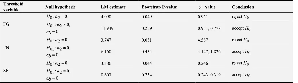
According to the above methods and steps, taking FG, FN, SF as threshold variables, and the basic measurement model (2) set up in this paper is formally tested. The results are in table 1.

Table 1. Formal Test of Model Setting.

Threshold

variable Null hypothesis LM estimate Bootstrap P-value

⌢

γ value Conclusion

FG

0: 2 0

H ω = 4.090 0.049 0.951 rejectH₀

01 2

3

: 0,

0

H ≠

= ω

ω 11.949 0.259 0.951, 0.778 acceptH0

FN

0: 2 0

H ω = 3.747 0.051 4.587 rejectH₀

01 2

3

: 0,

0

H ≠

= ω

ω 6.160 0.434 4.127, 1.826 acceptH0

SF

0: 2 0

H ω = 3.386 0.044 0.246 rejectH₀

01 2

3

: 0,

0

H ≠

= ω

ω 0.603 0.734 0.243, 0.319 acceptH0

It can be seen that when the model (2) takes FG and SF as threshold variables, at 5% significant level, there exists threshold effect and only a threshold variable, the model (2) conforms to the form (4). When FN is taken as the threshold variable, there exists threshold effect in model (2) at a significant level of 10%, and it also conform to model (4), that is, there is a threshold variable.

4.1.4. Co-Integration Test of Model Threshold

According to the previous test, the model (2) is substituted by the model (4) when FG, FN and SF are taken as threshold variables respectively. Furthermore, we can determine whether the model (4) is a threshold co-integration model by the statistical test ofC_FMOLSb i, . The test process is as follows: according to the threshold values in Table 1, the model (4) is estimated by completely modified ordinary least square estimation (FMOLS). Based on the estimated residual error, we can calculate the

,

b i FMOLS

C statistic by using partial residuals that mentioned by

Choi and Saikkonen [22], if the calculated Cb i_FMOLS, statistic is less than the critical value of its distribution (the critical value can be determined by Monte Carlo simulation experiment), then the model (4) is the threshold cointegration model. TheC_FMOLSb i, statistics are:

1 ₁

, 2 2 2 2

,

0

ˆ ( ˆ ) ( )

i b t b i

i u j

FMOLS

t i j i

C b

ω

u w s ds

+ − − −

= =

=

∑ ∑

⇒

∫

₍₇₎

Among them, bis the sample size of selected partial residuals, i is the starting point of partial residuals, FMOLSis the completely modified ordinary least square estimation, ωˆ_{i u}2_, is the consistent estimation of the long-term

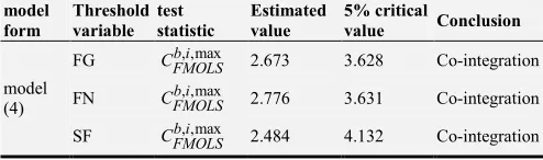
variance of u, andw s( )is the standard Brownian motion. The test results of model (4) are as follows (see Table 2).

Table 2. Co-integration Test of the Model Threshold.

model form

Threshold variable

test statistic

Estimated value

5% critical

value Conclusion

model (4)

FG Cb i_FMOLS, ,max 2.673 3.628 Co-integration

FN Cb i_FMOLS, ,max 2.776 3.631 Co-integration

SF Cb i_FMOLS, ,max 2.484 4.132 Co-integration

It can be seen from Table 2 that the model (4) is a threshold co-integration model with FG, FN and SF as threshold variable respectively, and the estimated values of

, ,max

b i FMOLS

C are less than the critical value at 5% significant level.

4.2. Findings

The threshold values in Table 1 are put into model (4), and estimated by FMOLS method respectively. The specific estimation results are obtained (see Table 3):

Table 3. Estimated Results of Model (4).

Basic Model Model (4)

Threshold Variabletv_t FG FN SF

Constant 0.6573 0.6440 0.6871

Mechanism 1 FG≤0.951 FN≤4.587 SF≤0.246

L

α 0.3219 0.3369 0.0359

K

β 0.7038 0.7048 0.6974

Mechanism 2 FG＞0.951 FN＞4.587 SF＞0.246

L

α －0.9546 －1.0712 0.2693

K

β 0.0033 0.0044 0.0018

As can be seen from Table 3, when the ratio of the FG, FN and SF reaches 0.951, 4.587, and 0.246 respectively, the industrial structure has different effects on the input efficiencies of capital and labor of economic growth. Specifically, when the ratio of output value of the tertiary industry to secondary industry is less than 0.951, that is, during 1979-2008, the capital and labor acted on economic growth with the first mechanism, that is, with the output elasticity of 0.7038 and 0.3219 respectively. During 2009-2015, this ratio was greater than 0.951, and the capital and labor acted on economic growth with combined action of the first and second mechanism, that is, with the output elasticity of 0.7071 and -0.6327 respectively. When the ratio of output value of the tertiary industry to that of primary industry was less than 4.587, that is, during 1979-2009, the capital and labor acted on economic growth with output elasticity of the first mechanism, namely 0.7048 and 0.3369, respectively. During 2010-2015, this ratio was more than 4.587, and the capital and labor acted on economic growth with combined action of the first and second mechanism, that is, with the output elasticity of 0.7092 and -0.7343 respectively. When the ratio of output value of productive service industry to the service industry was less than 0.246, that is, during 2003-2006 and 2010-2015, the capital and labor acted on economic growth with the first mechanism, that is, with the output elasticity of 0.6974 and 0.0359 respectively. During 1979-2002 and 2007-2009, this ratio was more than 0.246, and the capital and labor acted on economic growth with combined action of the first and second mechanism, that is, with the output elasticity of 0.6992 and 0.3052 respectively.

5. Conclusions

three industrial structure changes in China have undergone two profound changes to the economic growth. In the first profound change, when the proportion of the primary industry decreases and the proportion of the secondary industry and the third industry increases simultaneously, the factors of capital and labor act on economic growth with higher efficiency, but in the second profound change, when the proportion of the primary industry keeps declining while that of tertiary industry is close to and exceeds that of secondary industry, the output efficiency of capital remains basically unchanged, but the output efficiency of labor decreases dramatically, and the labor factor acts on economic growth with greater negative output elasticity. (iii) When the proportion of productive service industry within the tertiary industry drops below 0.246, the output efficiency of labor decreases significantly. The corresponding period is basically consistent with the period when the proportion of labor factors in the tertiary industry is close to or higher than that in the secondary industry, which leads to the decline of productivity of labor factors. This shows that the proportion of producer services in the tertiary industry is basically the same. This indicates that the decline of the ratio of the productive service industry in the tertiary industry and the structural change that the proportion of the tertiary industry is close to and exceeds the proportion of the secondary industry lead to the decline of China's economic growth efficiency in the period from 2009 to 2010.

6. Explanation of China's Recent

Economic Deceleration from the

Perspective of Industrial Structure

Change

The classical studies at home and abroad show that in the process of economic growth or industrialization, it is inevitable to accompany the change of industrial structure, that is, the leading industry of national economy is gradually transforming from the primary industry to the secondary industry, and then to the tertiary industry. The reason is that the change of industrial structure leads to the gradual flow of labor factors from the low efficient industrial sectors to the high efficient sectors, which leads to the great improvement of labor productivity and the sustained promotion of economic growth. With regard to China's practice, the industrialization process since China's reform and opening up also follows this evolution law of industrial structure, but after 2009-2010, when China's industrialization process entered the middle and late stage, although the evolution law of the three industrial development still maintained the above trend, the output efficiency of labor reversed greatly, that is, from the larger positive output elasticity in the previous stage to the larger negative output elasticity.

Looking at the total input of labor factors and the distribution of the three industrial structures in China after 2009-2010, it can be found that the total input of labor factors and the change trend of labor force in the primary industry remain basically unchanged, that is, the total amount of labor

input remains increasing year by year, and the labor input of the primary industry is still decreasing year by year, the labor input of the tertiary industry is still increasing year by year, but the labor input of the second industry has changed from increasing year by year to decreasing year by year. The labor force in the tertiary industry is still increasing year by year, but the total amount of labor force in the tertiary industry has exceeded that in the secondary industry. This phenomenon shows that the distribution of industrial structure of China's labor force has undergone great changes in recent years, it has changed from the former secondary industry adsorbing labor force to the tertiary industry adsorbing labor force. Furthermore, combined with the analysis of the internal structure changes of the tertiary industry, the proportion of productive service industry has been decreasing in recent years, which shows that a large amount of labor adsorbed by the tertiary industry mainly flows to the non-productive service industry with low labor efficiency, and this pulls down the average labor productivity of the whole service industry. To sum up, China's industrialization has not been completed since the reform and opening up, and it is too early for the industrial structure changed to the service industry, along with the excessive non-productive development of the industrial structure in the tertiary industry, therefore, the efficiency of labor factors has dropped dramatically, which is one of the important reasons why China's economy has slowed down in recent years and relied too much on investment.

7. Policy Proposals

in China 2025" as an opportunity to improve the innovative and basic ability of manufacturing industry, and promote the deep integration of information technology and manufacturing technology as well as promote the high-end and intelligent development of manufacturing industry. Third, vigorously cultivate and develop strategic emerging industries. Strategic emerging industries are the result of the continuous deepening and integration of emerging technology and industrial industry. Promoting the development of strategic emerging industry can further enhance the efficiency of labor factors in the whole society. Fourth, we should focus on promoting the development of productive service industry. The productive service industry is dependent on the development of the second industry, which is the transition and convergence industry of the transformation of the secondary industry to the tertiary industry. Because productive service industry has higher technological content, it maintains the continuity of higher labor efficiency of secondary industry and vigorously develops productive service industry in the middle and late stage of industrialization and conforms to the trend of industrial structure development.

Fifth, properly develop the living service industry. Compared with the emerging manufacturing and productive service industry, the labor productivity of the living service industry is lower. However, the proper development of the living service industry in the middle and late stage of industrialization can not only meet the needs of enriching people's livelihood in the current development stage, but also have no obvious drag effect on the current labor productivity, meanwhile, to a certain extent, it also maintains the trend of the industrial development in the post-industrialization stage.

Acknowledgements

This research was supported by the National Social Science Foundation of China (No. 16BJY009).

References

[1] Lang, L. H., Chou, M. S (2012). Structural reform and macroeconomic Stability. Economic Research 8, 152-160. [2] Liu, S. X., Fan, Y. X (2012). Macroeconomic policy should be

dominated by structural reform. Chinese Finance 20, 71-73. [3] Liu, Y. N., An, L. R., Jin, T. L (2014). The quality of China's

economic growth under the background of unbalanced economic structure. Research on Quantity Economy and Technology Economy 10, 20-35.

[4] Yuan, F. H (2014). Analysis of the dual structure of Chinese economy. Economic and Management Review 3, 9-17. [5] Yu, B. B (2015). The Economic growth effect of industrial

structure adjustment and productivity improvement: an analysis based on Chinese urban dynamic spatial panel model. Industrial Economy of China 12, 83-95.

[6] Shen, K. R., Teng, Y. L (2013). Economic growth in China under the “structural” deceleration. Economist 8, 29-38. [7] China Economic Growth Frontier Group (2013). Structural

characteristics, transition risk and ways to improve efficiency for slowdown of China's economic. Economic Research 3, 4-18.

[8] Denison, E. F (1962). United States economic growth. Journal of Business 35 (2), 109-121.

[9] Peneder, M. (2003). Industrial structure and aggregate growth. Structural Change & Economic Dynamics, 14 (4), 427-448. [10] Kuznets, S (1971). economic growth of nations, Harvard

University Press.

[11] Chenery, H. B., Robinson, S., Syrquin, M., et al (1986). Industrialization and growth: a comparative study. Oxford University Press.

[12] Nutahara, K (2008). Structural changes and economic growth: evidence from Japan. Economics Bulletin 15 (9), 1-11. [13] Cortuk, O., Singh, N (2013). Analyzing the structural change

and growth relationship in India: state-level evidence. Working Papers, UC Santa Cruz Economics Department, No. 712.

[14] Cao, K. H., Birchenall, J. A (2013). Agricultural productivity, structural change, and economic growth in post-reform China. Journal of Development Economics 104 (3), 165-180. [15] Donatella, S (2015). Structural change, globalization and

economic growth in China and India. European Journal of Comparative Economics 12 (2), 133-163.

[16] Liu, W., Zhang H (2008). Changes in industrial structure and technological progress in China's economic growth. Economic Research 11, 4-15.

[17] Gan, C. H., Zheng, R. G., Yu, D. F (2011). The influence of China's industrial structure change on economic growth and fluctuation. Economic Research 5, 4-16.

[18] Chou, S. F., Wang, W., Dong, D. X (2013). An Analysis of the effect of human capital and industrial structure transformation on economic growth: empirical evidence from provincial panel data in China. Research on Quantity Economy and Technology Economy 8, 65-77.

[19] Kumar, N (2002). Globalization and the quality of foreign direct investment. Oxford University Press.

[20] Gonzalo, J., Pitarakis, J (2006). Threshold effects in cointegrating relationships. Oxford Bulletin of Economics and Statistics 68 (s1): 813-833.

[21] Teräsvirta, T (1994). Specification, estimation, and evaluation of smooth transition autoregressive models. Journal of the American Statistical Association, 89 (425): 208-218.