A comparative study between two numerical solutions of the Navier-Stokes equations

(1)

1

*_{Corresponding author}

A comparative study between two numerical solutions

of the Navier-Stokes equations

M. Alemi* and R. Maia

Departamento de Engenharia Civil, Faculdade de Engenharia, Universidade do Porto, Rua Dr. Roberto Frias, s/n, Porto 4200-465, Portugal

Article info: Abstract

The present study aimed to investigate two numerical solutions of the Navier-Stokes equations. For this purpose, the mentioned flow equations were written in two different formulations, namely (i) velocity-pressure and (ii) vorticity-stream function formulations. Solution algorithms and boundary conditions were presented for both formulations and the efficiency of each formulation was investigated by considering a two-dimensional low laminar flow around a square pile in a rectangular computational domain. Simulations under the same conditions were conducted to assess the difference between results generated by both formulations. Furthermore, the accuracy of the results was analyzed through a comparison of the results with the available reference data. In addition, computational efficiency of both formulations was investigated in term of computation time. The corresponding results indicated that both formulations are adequate to the case used in the present study. Moreover, performed simulations showed that solving the vorticity-stream function form of the flow equations is faster than solving the velocity-pressure form of those equations for simulating a two-dimensional laminar flow around a square pile.

Received: 16/11/2016 Accepted: 11/09/2016 Online: 03/03/2017

Keywords:

CFD, Laminar, Navier-Stokes, Square Pile, Velocity-Pressure,

Vorticity-Stream function.

Nomenclature

Stream-wise direction (x) Pressure Span-wise direction (y) Vorticity

, Velocity components (u,v) Stream function

∗_, ∗ _{Intermediate velocities} _{Iteration number}

Dynamic viscosity of fluid Time step counter Fluid density ∆ Time step size

h Grid spacing Over relaxation parameter

D Square side dimension Recirculation length

Uin Inlet flow velocity i, j Node indexes

Re Reynolds number (ρUinD

μ ) CDP Pressure drag coefficient (

(2)

JCARME M. Alemi, et al. Vol. 6, No. 2

2

1. Introduction

Nowadays, numerical methods such as computational fluid dynamics (CFD) are widely used in engineering to perform a full analysis on the flow characteristics around bluff bodies. The CFD methods can be classified in accordance with the used solution algorithms. In order to choose a solution algorithm, numerical accuracy and computation time are important factors. Therefore, a balance of these factors is required in any numerical simulation. The governing equations to predict the flow behavior around a pile are the Continuity and the Navier-Stokes equations. One difficulty for solving the mentioned flow equations is that there is no explicit equation for the pressure. Several methods have been proposed to solve this problem, e.g., SIMPLE (Semi-Implicit Method for Pressure Linked Equations) and Fractional time step methods.

The SIMPLE method was firstly proposed by Patankar and Spalding [1]. Extensions were then added to the method: SIMPLER (SIMPLE Revised), SIMPLEC (SIMPLE Consistent) and PISO (Pressure-Implicit with Splitting of Operators). A good description of the SIMPLE method and its extensions has been presented by Versteeg and Malalasekera [2]. Another method to solve the flow equations is the Fractional time step which was firstly introduced by Chorin [3]. Then, various forms of this method were investigated and developed by several researchers (e.g. Kim and Moin [4] among others). Majander and Siikonen [5] compared two mentioned methods and noted that the Fractional time step method is faster than the SIMPLE method at low Reynolds number range.

In these mentioned methods, unknown variables are the velocity components and the pressure (primitive variables). The flow equations can also be written in the vorticity and stream function form such that the pressure is absent in the main flow equations. A good

explanation on this formulation can be found in [6, 7].

In the present study, two mentioned formulations of the flow equations (velocity-pressure and vorticity-stream function formulations) were employed and their efficiency was investigated by considering a two-dimensional (2-D) flow around a square pile at low laminar flow conditions.

In the following sections, firstly, the problem geometry is defined and then the governing equations are expressed in primitive variables and vorticity-stream function formulations. Afterward, the corresponding solution algorithms are explained properly and finally, numerical results are presented and analyzed.

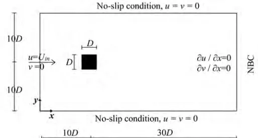
2. Computational domain

In the present study, a rectangular domain (40D×20D) was used to simulate the flow past a stationary 2-D square pile as shown in Fig. 1. The computational domain was discretized into a uniform grid with equal grid spacing (h) in both x and y directions. The square pile was modeled by blocking cells inside the square geometry. The inlet boundary section was located 10D upstream from the center of the square and the fluid flow down from this boundary was considered to have a specified constant velocity (free-stream). That distance is necessary to obtain results independent of the inlet location for the mentioned flow conditions [8]. Lateral boundaries were located far away

(10D) from the square pile to reduce probable

effects of the boundaries on the flow behavior around the square. The no-slip condition was imposed at the lateral boundaries and also at the pile surface. Finally, the Neumann boundary

condition (NBC), 𝜕𝑢/𝜕𝑥 = 𝜕𝑣/𝜕𝑥 = 0, was

(3)

JCARME A comparative study between . . . Vol. 6, No. 2

3

Fig. 1. Computational domain and boundary conditions.

3. Velocity-Pressure formulation (u, v-p)

The incompressible Continuity and Navier-Stokes (or momentum) equations in the velocity-pressure form can be written as Eqs. (1) and (2).

= 0

(1)

+

= −

1 +

(2)

As mentioned in Introduction, lack of explicit equation for the pressure is a major problem to solve the main flow equation. Hence, in the present study, a simple form of the Fractional time step method was employed to solve the flow equations. In this simple method, the intermediate velocities are calculated by ignoring the pressure terms in the momentum equations. Then, the pressure values are obtained by solving the Continuity equation for each grid cell. Finally, the intermediate velocities are corrected using the pressure values.

For computing the intermediate velocities, the second-order-explicit Adams-Bashforth scheme, as explained in [7], was used for treating the convection and diffusion terms of the Navier-stokes equations. In addition, the central difference scheme was employed to approximate the spatial derivatives of the flow equations. Therefore, the present algorithm is second-order accurate in both space and time.

Since the convection and diffusion terms are solved explicitly, stability consideration for a 2-D convective-diffusive equation requires the time step to satisfy [9]:

∆ ≤

ℎ

4 ,

2 (

+

)

(3)

The first term on the right-hand side of Eq. (3) is related to the diffusion terms and the other term is related to the convection terms.

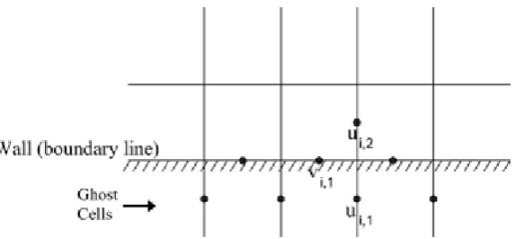
The discretization of the flow equations was performed on a staggered grid system such that the velocities are calculated on the vertical cell interfaces, the velocities on the horizontal cell interfaces and the pressure ( ) in the center of each cell. In other words, the velocities and pressure are computed at different locations. A direct advantage of using the staggered grid system is that the pressure boundary conditions are not required in the calculations.

The adopted control volume definition for u, v velocity components and the pressure are presented in Fig. 2 (a, b and c), respectively. Applying the Continuity equation to the control volume related to the pressure variable results to a relation between the pressure and the intermediate velocities as Eq. (4):

,

+

,

+

,

+

,

− 4

_,

=

ℎ

∆

∗ ,

−

∗ _,

+

∗ _,

−

∗ _,

(4)

4

Equation (4) is an implicit equation; hence, the iterative Successive Over Relaxation (SOR) method, as explained in [7], was employed to solve this equation in the present study.

Applying the correct boundary conditions in the staggered grid system is complex and requires care, as some boundary points lie exactly on the boundary lines while others are out of those (Fig. 3). At the points that lie exactly on the boundary lines, the values are directly prescribed (such as 𝑢 at the inlet section and 𝑣

at the lateral boundary lines). For other boundary points, the average value of two neighbor points on the boundary line should satisfy the boundary condition. In order to exemplify that, two points are considered below

and above a wall boundary similar to Fig. 3. The average value of data on these two points should be equal to the u-velocity at the wall boundary. For a wall with the no-slip condition, u-velocity is equal to zero. Hence:

𝑢

_𝑖,1

+ 𝑢

_𝑖,2

2 = 0 → 𝑢

𝑖,1

= − 𝑢

𝑖,2

(5)

It is noteworthy to mention that the pressure values are not required in the so-called ghost cells (see Fig. 3) but the pressure equation, Eq. (4), should be modified in the cells close to the boundary lines according to the velocity values at these lines.

(a) (b) (c)

Fig. 2. Control volume for: (a) u-velocity, (b) v-velocity components, and (c) pressure.

(5)

5

4. Vorticity-Stream function formulation (

ω-𝜓)

Summing up the 𝑥- and 𝑦- direction

components of the momentum equations, each multiplied, respectively, by (− ∂/ ∂y) and (∂/ ∂x), leads to the incompressible

Navier-Stokes equations in the vorticity-stream function form (without the pressure term) as follows:

𝜕𝜔

𝜕𝑡

+ 𝑢

𝜕𝜔

𝜕𝑥

+ 𝑣

𝜕𝜔

𝜕𝑦

=

𝜇

𝜌

[

𝜕

2

𝜔

𝜕𝑥

2

+

𝜕

2

𝜔

𝜕𝑦

2

]

(6)

where 𝜔 is the vorticity and defined as:

𝜔 =

𝜕𝑣

𝜕𝑥

−

𝜕𝑢

𝜕𝑦

(7)

In accordance with the Continuity equation, stream function (𝜓) is defined as follows:

𝑢 =

𝜕𝜓

𝜕𝑦

(8)

𝑣 = −

𝜕𝜓

𝜕𝑥

(9)

Substituting Eq. (8) and Eq. (9) into the definition of the vorticity, Eq. (7), leads to:

𝜕

2

_𝜓

𝜕𝑥

2

+

𝜕

2

_𝜓

𝜕𝑦

2

= −𝜔

(10)

Equation (6) can be solved using an explicit or an implicit method. In the present study, this equation was discretized by the explicit Adams-Bashforth scheme in time and the central difference scheme in space. Equation (10) can be solved by an iterative method or even by a direct solution. In the present study, the iterative SOR method was employed to solve the mentioned equation. By that, Eq. (10) yields as:

𝜓

_𝑖,𝑗𝑘

=

1

4 𝛽(𝜓

𝑖+1,𝑗

𝑘−1

_{+ 𝜓}

𝑖−1,𝑗𝑘

+ 𝜓

𝑖,𝑗+1𝑘−1

+ 𝜓

_{𝑖,𝑗−1}𝑘

+ ℎ

2

𝜔

𝑖,𝑗

)

+ (1 − 𝛽) 𝜓

_𝑖,𝑗𝑘−1

(11)

where 𝜓𝑘 is the kth approximation or iteration

of 𝜓 at each time step. The over relaxation

parameter is denoted by 𝛽 and a good choice of

this parameter can speed up the convergence. In order to solve the Navier-Stokes equations in the form of the vorticity and stream function, all variables were calculated at the intersection of the grid lines. Initial and boundary conditions were firstly set at all internal and cell boundary points and then vorticity, stream function and velocity components were computed at each new time step (n+1), as follows:

* Calculation of the vorticity at each internal point at time step (n+1) using Eq. (6) * Computation of the stream function using Eq.

(11)

* Updating the velocity components through Eqs. (8) and (9)

* Updating the boundary values

The square geometry and the grid cells inside the square are presented in Fig. 4. These cells are blocked to model the square pile geometry in the present study. Points A, B, C and D are defined as square corner points.

The no-slip boundary condition was imposed at the square faces AB, BC, CD, and AD. Therefore, velocity components are equal to zero at each grid points on the mentioned faces. In order to satisfy the no-slip condition, the stream function should be constant on the square faces. Liu and Wang [6] noted that the stream function is constant on the square faces but varies with time for the calculations of the unsteady flows. In the present study, the steady-state case, 𝜓pile was considered equal to zero.

In order to determine the vorticity (𝜔), Taylor

series for stream function were written up to the second order term like Eq. (12) for the face BC:

𝜓

𝑖,𝑗𝑚𝑎𝑥+1

= 𝜓

𝑖,𝑗𝑚𝑎𝑥

+ ℎ (

𝜕𝜓

𝜕𝑦

)

_{𝑖,𝑗𝑚𝑎𝑥}

+

ℎ

2

2 (

𝜕

2

_𝜓

𝜕𝑦

2

)

+ ⋯

(6)

6

Applying the no-slip boundary condition leads to Eq. (13):

𝜔

_{𝑖,𝑗𝑚𝑎𝑥}

=

2 ℎ

2

(𝜓

− 𝜓

_{𝑖,𝑗𝑚𝑎𝑥+1}

)

(13)

Fig. 4. A part of the computational domain, ω-𝜓

formulation.

In order to compute the pressure values that may be required to compute the pressure force acting on the square pile, the momentum equations, Eq. (2), should be solved at the square faces as explained in [7].

5. Results and discussion

Two computational codes (using the Finite difference method) were developed by employing two different formulations (u,v-p

and 𝜔-𝜓) as explained in section 3 and section

4. The numerical codes were then run for various Reynolds numbers (10, 20, 30 and 40) using the same uniform grid spacing of 0.1 and the time step size of 0.01, both dimensionless. In both formulations, computations were repeated at each new time step until the maximum error (the difference between obtained values at new time step and the previous one) went below the convergence limit (10-6_{, in the present study).}

The pressure distribution around the square pile, computed by u, v-p formulation, is presented in Fig. 5. The maximum pressure is observed at the center of face AB (stagnation point) and the minimum values are detected close to the square corner points A and B as pictured in Fig. 5. As the Reynolds number increases, the pressure value at the stagnation point decreases and

consequently the pressure force acting on the pile changes. One important parameter of the flow around a square pile is the drag force produced by the viscous (friction) and pressure forces acting on the square pile. In the present study, the pressure drag coefficient (

C

DP) is

presented in Fig. 6 together with the corresponding numerical results obtained by Sharma and Eswaran [10]. They defined a

rectangular computational domain (26D×20D)

such that the square center was located 9D from the inlet boundary section. They also considered the lateral boundaries 10D from the square center (as in the present study) and noted that in this case, the boundaries are sufficiently far away and their presence has little effect on the characteristics of the flow near the square. These researchers employed the Convective boundary condition (CBC) at the outlet boundary section while the Neumann boundary condition (NBC) was used in the present study. Sohankar et al. [8] have investigated these mentioned outlet boundary conditions and concluded that the minimum downstream length of the pile (XDown) for negligible

near-body effects is much lower with the CBC than with the NBC. As an example, on comparing NBC and CBC, both with Re=100: CBC essentially shows the same global results for

XDown=10D, as the NBC for XDown=26D. This

may justify the difference between the length of the computational domain used in the present

study (40D) and what was used by Sharma and

Eswaran (26D) [10].

Overall, there is a good agreement between the numerical results (

C

DP) obtained by u,v-p

formulation in the present study and those obtained numerically by Sharma and Eswaran [10]. Moreover, Fig. 6 also shows that the pressure drag coefficient varies strongly with Reynolds number in the steady-state flow regime.

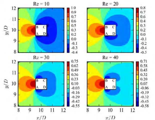
The predicted flow behavior around the square pile is presented in Fig. 7 by drawing the streamlines and the velocity vectors for ω-𝜓

and u, v-p formulations, respectively. At values of the Reynolds number used in the present study (10 ≤ Re ≤ 40), the flow field around

(7)

7

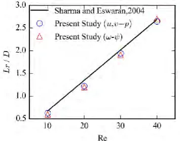
behind the pile rises in length with increasing

Reynolds number. All the pictures in Fig. 7 indicate that the flow separates at the trailing edge and reattaches at a short distance downstream of the square. The stream-wise distance from the rear face of the square to the re-attachment point along the wake centerline is denoted by 𝐿𝑟 (recirculation length). In order to

assess the accuracy of the obtained numerical results, the corresponding non-dimensional recirculation lengths (𝐿𝑟⁄𝐷) are compared with

those obtained numerically by Sharma and Eswaran [10] as shown in Fig. 8. Sharma and

Eswaran presented the following expression (Eq. (14)) to compute the recirculation length (with a maximum deviation of 5%):

Lr

D = 0.0672 × Re, 5 ≤ 𝑅𝑒 ≤ 40

(14)

Single point plots in Fig. 8 indicate that the numerical predictions computed by both formulations agree well, and also fit fairly well with the results obtained numerically by Sharma and Eswaran [10].

Fig. 5. Non-dimensional pressure ( 𝑃

𝜌 𝑈_𝑖𝑛2) around the square pile at different Reynolds numbers.

(8)

8

Fig. 7. Flow behavior around the square pile for various Reynolds numbers; Left: ω-𝜓 formulation, Right: u,v-p

formulation.

(9)

9

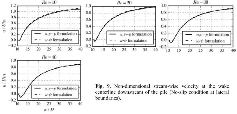
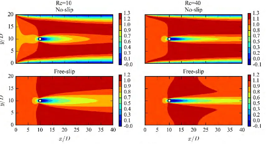
The stream-wise velocity ( ⁄ ) at the wake

centerline downstream of the pile is presented in Fig. 9 for both formulations. There is a good agreement between the results obtained by two formulations used in the present study. The u -velocity on the centerline is zero at the square surface. It reaches a negative minimum value in the recirculation zone and then increases progressively until a maximum value. Furthermore, it can be observed that the u -velocity values at the wake centerline decrease with increasing Reynolds number because they are influenced by the wake region, and the length of the wake region increases with Reynolds number. Moreover, it is observed that the u -velocity at the outlet section is 10% higher than the inlet velocity for Re=10. In order to justify that difference, the u-velocity values were also calculated by considering the free-slip condition ( = 0, / = 0) at the lateral boundaries and compared with those obtained by employing the no-slip condition ( = = 0) in Fig. 10 and Fig. 11. The obtained numerical results show that the outlet u-velocity is 20% lower than the inlet velocity, for Re=10, when the free-slip condition was used in the solution, although the u-velocity values are nearly the same close to the square for both mentioned boundary conditions (see Fig. 11).

In the case of using the no-slip condition at lateral boundaries, a boundary layer forms near each mentioned boundary and its thickness

becomes larger with decreasing Reynolds number. Therefore, the no-slip boundary condition at the lateral boundaries can be effective to accelerate the velocity at the outlet section in this case.

In the present study, the computation time (CPU time) was also analyzed to assess the efficiency of two formulations. At the first stage, initial velocity components, vorticity and stream function, were set equal to zero. The corresponding CPU time and the number of time steps to obtain the steady-state results are presented in Table 1. Furthermore, in the second stage, u-velocity was considered equal to the inlet flow velocity only for u, v-p formulation as the initial condition (u=Uin, v=0). The corresponding results are also presented in Table 1.

The obtained results show that the initial condition affects the number of inner iterations (SOR method) and also the total number of time steps required to achieve the steady-state results in u, v-p formulation. When initial u-velocity was changed from zero to Uin, the u, v-p formulation became approximately 1.5 times faster, while the results were nearly the same (less than 0.1% deviation). Nevertheless, the

formulation was still much faster than u, v-p formulation for simulating 2-D laminar flow based on the algorithms used in the present study.

(10)

10

Fig. 10. The stream-wise velocity in the whole computational domain for different lateral boundary conditions.

Fig. 11. The stream-wise velocity at the wake centerline for different lateral boundary conditions.

Table 1. Comparison of the CPU time and number of time steps for u,v-p and ω- 𝜓 formulations.

𝝎-𝝍 formulation u, v-p formulation

Re No. Time _Steps CPU Time (s) _{u=0, v=0}No. Time Steps _u=U CPU Time (s)

in, v=0 u=0, v=0 u=Uin, v=0

10 6188 143 4579 4363 2972 2029 20 7017 142 4898 4764 3048 1978 30 6859 139 5089 5026 3191 1872 40 16552 210 5413 5316 3147 1892

Finally, in the third stage, the steady-state results were considered as initial data and two mentioned formulations were solved just for one

(11)

11

corresponding CPU time was 3.125 × 10-2 and

6.25 × 10-2 seconds for the ω-𝜓 and u, v-p

formulations, meaning that, after achieving the steady-state results, the ω-𝜓 formulation is still

two times faster than the u, v-p formulation. This can be due to the fact that in the ω-𝜓

formulation, fewer equations are solved at each time step.

It should be noted that in a 2-D case, the primitive variable (u, v-p) formulation requires three unknown parameters in contrast to the single stream function and vorticity. But in a three-dimensional case (Re>190 for the circular cylinder [11]), the primitive variable formulation has four unknowns, while the 𝜔-𝜓 formulation

has three components for vorticity and three for vector stream function [12, 13].

6. Conclusions

In the present study, the flow behavior around a two-dimensional square pile was simulated employing two different formulations of the Navier-Stokes equations, namely (i) velocity-pressure and (ii) vorticity-stream function. A staggered grid system was used in the first method, whereas in the latter method, all variables (u, v, 𝜔 and 𝜓) were calculated at the

same location (intersection of the grid lines). Computational domain, the location of the square pile, grid spacing and boundary conditions were considered the same for both formulations.

Using the Finite difference method, two mentioned formulations were solved for various Reynolds numbers (10~40). Both formulations could present nearly the same results. Moreover, both formulations were shown to be adequate to study the present 2-D case with a reasonable accuracy. Performed simulations did also show that the vorticity-stream function formulation is faster than the velocity-pressure formulation. Nevertheless, the pressure term is absent in the vorticity-stream function formulation and that is often required in engineering studies.

References

[1] S. V. Patankar, and D. B. Spalding, “A

calculation procedure for heat, mass and momentum transfer in three-dimensional

parabolic flows,” Int. J. Heat Mass

Transf., Vol. 15, No. 10, pp. 1787-1806, (1972).

[2] H. K. Versteeg, and W. Malalasekera, An

Introduction to Computational Fluid Dynamics - The Finite Volume Method. Longman Scientific & Technical, (1995).

[3] A. J. Chorin, “Numerical solution of the

Navier-Stokes equations,” J. Math.

Comput.,Vol. 22, No. 104, pp. 745-762, (1968).

[4] J. Kim, and P. Moin, “Application of a Fractional-step method to incompressible

Navier-Stokes equations,” J. Comput.

Phys., Vol. 59, No. 2, pp. 308-323, (1985).

[5] P. Majander, and T. Siikonen, “A

comparison of time integration methods in an unsteady low-Reynolds-number flow,” Int. J. Numer. Methods Fluids, Vol. 39, No. 5, pp. 361-390, (2002).

[6] J.-G. Liu, and C. Wang, “High order

finite difference methods for unsteady incompressible flows in multi-connected domains,” J. Comput. Fluids, Vol. 33, No. 2, pp. 223-255, (2004).

[7] S. Biringen, and C.-Y. Chow, An

introduction to computational fluid mechanics by example. John Wiley & Sons, (2011).

[8] A. Sohankar, C. Norberg, and L.

Davidson, “Low-Reynolds-number flow around a square cylinder at incidence: Study of blockage, onset of vortex shedding and outlet boundary condition,”

Int. J. Numer. Methods Fluids, Vol. 26, No. 1, pp. 39-56, (1998).

[9] J. F. Ravoux, a. Nadim, and H.

Haj-Hariri, “An embedding method for bluff body flows: interactions of two

side-by-side cylinder wakes,” Theor. Comput.

Fluid Dyn., Vol. 16, No. 6, pp. 433-466, (2003).

[10] A. Sharma, and V. Eswaran, “Heat and fluid flow across a square cylinder in the two-dimensional laminar flow regime,”

Numer. Heat Transf. Part A Appl., Vol. 45, No. 3, pp. 247-269, (2004).

(12)

12

around two circular cylinders in tandem,” J. Fluids Struct., Vol. 22, No. 6-7, pp. 979-988, (2006).

[12] E. Weinan, and L. Jian-Guo, “Finite difference methods for 3D viscous incompressible flows in the vorticity-vector potential formulation on

nonstaggered grids,” J. Comput. Phys., Vol. 138, No. 1, pp. 57-82, (1997). [13] T. Hou, and B. Wetton, “Stable

fourth-order stream-function methods for incompressible flows with boundaries,” J. Comput. Math., Vol. 27, No. 4, pp. 441-458, (2009).

How to cite this paper:

M. Alemi and R. Maia, “A comparative study between two numerical solutions of the Navier-Stokes equations”, Journal of Computational and Applied Research in Mechanical Engineering, Vol. 6. No. 2, pp. 1-12

DOI: 10.22061/jcarme.2017.580