DEEPWATER PRODUCTION FORECASTING USING COMPUTATIONAL
INTELLIGENCE TECHNIQUES
*Osunleke, A.S. and Oladoyin, O.O.
Department of Chemical Engineering,
Obafemi Awolowo University, Ile-Ife 220005, Osun State, Nigeria.
E-mail: [email protected] and E-mail: [email protected];
ABSTRACT
Precise and consistent production forecasting is indeed an important step for the management and planning of petroleum reservoirs. This research work is aimed at developing a new neural approach to forecast cumulative oil production. The methodology employed is using a neural network with its weight optimized with genetic algorithm (NN-GA). NN-GA overcomes the limitation of the conventional neural networks of settling in a local minima by optimizing the weights and biases to be used to initialize a Nonlinear Autoregressive Neural Network with Exogenous Input (NARX). Thus, NN-GA possesses a great potential in forecasting petroleum reservoir productions without sufficient training data. A pre-processing procedure was employed in order to reduce measurement noise in the production data from the oilfield by normalizing the raw data using z-core normalization technique and optimal network topology selection using correlation functions (CCF). Simulation studies were carried out on a deepwater reservoir located off the coast of the Niger-Delta in Nigeria, to prove the efficacy of the NN-GA in forecasting cumulative oil production of the field with data available. The results of these simulation studies indicate that the NN-GA model has a good forecasting capability with high accuracy to predict cumulative oil production and this was compared to the widely used Decline Curve Analysis technique. It was concluded that the NN-GA procedure has a very good potential to be applied to petroleum forecasting and the possibility of including more reservoir production parameters to the model to help for better accuracy and precision in the forecasting process.
Keywords: NARX Neural Network, Genetic Algorithm, Optimization, Decline Curve Analysis, Time series forecasting
INTRODUCTION
The increasing search for oil and gas reserves has led to the movement of these exploration activities steadily away from land locations and moving farther offshore to deepwater environments. 60% of the world’s oil discoveries were found in deep water in the past 10 years.
The oil and gas industry has always relied on production forecasts to predict the profitability of producing oil/gas facilities. Production forecasts are also used to determine the life span of a producing oil/gas facility. This is determined by estimating the time that the production forecast reaches a pre-defined economic limit.
In the past, several forecasting methods have been developed from decline curve analysis to soft computing techniques.[1].
The reservoir is described by a set of time series (TS) of fluids from petroleum wells, which are characterized by different starting points and mutual influence. Production performance is both controlled by the reservoir properties and is also affected by operational constraints and surrounding wells performance. The rock and fluid properties of the reservoirs are highly nonlinear and heterogeneous in nature.
Time Series (TS) forecasting, along with clustering and classification, is one of the traditional time series data mining tasks[3].
Most of the existing decline curve analysis techniques are based on the empirical equations including exponential, hyperbolic, and harmonic equations[4]. However, the problem with this technique is that it is difficult to identify which equation describes the production of a reservoir. In addition, a single curve often cannot describe the entire life of a reservoir, and curve fitting not only makes the matching process difficult but also results in unreliable predictions[5].
Computational Intelligence (CI) techniques are adaptive mechanisms to enable or facilitate intelligent behavior in complex and changing environments. They include aspects of artificial intelligence that exhibit an ability to learn or adapt to new situations, to generalize, abstract, discover and associate[6]. According to[6], CI techniques are broadly classified into five main groups, namely; artificial neural networks (NN), evolutionary computation (EC), swarm intelligence (SI), artificial immune systems (AIS), and fuzzy systems (FS).
NN is an especially efficient algorithm to approximate any function with finite number of discontinuities by learning the relationships between input and output vectors [7]. These algorithms can learn from the experiments, and also are fault tolerant in the sense that they are able to handle noisy and incomplete data. The ANNs are able to deal with nonlinear problems, and once trained can perform prediction and generalization at high speed [8]. They have been used to solve complex problems that are difficult for conventional approaches, such as control, optimization, pattern recognition, classification, properties and desired that the difference between the predicted and observed (actual) outputs be as small as possible[7].
Evolutionary computation (EC) has as its objective to mimic processes from natural evolution, where the main concept is survival of the fittest; [6]an example of EC is Genetic algorithms (GA) which model genetic evolution.
Swarm intelligence (SI) originated from the study of colonies, or swarms of social organisms. Studies of the social behavior of organisms (individuals) in swarms prompted the design of very efficient optimization and clustering algorithms[6].
An artificial immune system (AIS) models some of the aspects of a natural immune system, and is mainly applied to solve pattern recognition problems, to perform classification tasks, and to cluster data[6].
Fuzzy sets and fuzzy logic allow what is referred to as approximate reasoning. With fuzzy
sets, an element belongs to a set to a certain degree of certainty. Fuzzy logic allows reasoning with these uncertain facts to infer new facts, with a degree of certainty associated with each fact[6].
Artificial intelligence tools have been extensively applied in petroleum industries because of their potential to handle the nonlinearities and time-varying situations[9]. Neural networks (NN) is one of the most attractive methods of artificial intelligence to cope with the nonlinearities in production forecasting[2] as well as in parameters estimation [10] due to its ability to learn and adapt to new dynamic environments. Numerous researches have shown successful implementation of NN in the field of oil exploration and development such as pattern recognition in well test analysis [11], reservoir history matching[12], prediction of phase behavior [13]prediction of natural gas production in the United States [14]and reservoir characterization [9] by mapping the complex nonlinear input–output relationship.
2. NEURAL NETWORK
They were made of a large number of simple computing components, called nodes or neurons that arranged to form an input layer, one or more hidden layers and an output layer [7].
They further include interconnections between the nodes of successive layers through the so-called weights [15]. The role of these weights is to modify the signal carried from one node to the other and enhance or diminish the influence of the specific connection. Each neuron in the hidden layer receives weighted inputs from each neuron in the previous layer plus one bias [15][16].The internal weights of the network are adjusted in the course of an iterative process termed training. There exist many network architectures but Multilayer Perception is the most popular among them. The number of nodes in the feed forward neural network input layer is equal to the number of inputs in the process, whereas the number of output nodes is equal to the number process output[16, 17].
Essentially, the training procedure is intended to obtain an optimal set of the network weight, which minimizes an error function. The commonly employed error function is theme an squared error (MSE) as defined by:
= 1
2 ( ) − ( )
respectively. Generally, minimizing the MSE is the priority of training a NN.
Fig. 1: Schematic of a typical feedforward neural network
3. GENETIC ALGORITHM
In this work Genetic Algorithm (GA) was used due to its good capacity for searching in high dimensions. Genetic algorithm is based on natural evolution through selection. Each individual in a population is represented by its chromosome, traditionally composed by bit strings (binary). Each chromo some represents a solution to a problem and each of them has a fitness value which measures its quality numerically.
The reproduction process consists basically of selection, crossover and mutation.
First an initial population of size N (number of individuals) is defined. This population is ranked by fitness values and elite individuals are selected. These individuals are subjected to crossover and mutation process where a new generation of individuals, potentially superior is generated. This procedure (one generation or iteration) is repeated till a stop pingcriterion is reached.
In the crossover process genes (feature) from parents (individuals) are extracted and recombined into a potentially superior child [18]. Crossover rate is used to control the intensity of its occurrence. High rates make the population to converge to the elite individuals quickly. The mutation process adds diversification in the reproduction process. One individual can suffer some modification in its gene and generate a new different individual. Its occurrence is controlled by a usually low value of mutation probability.
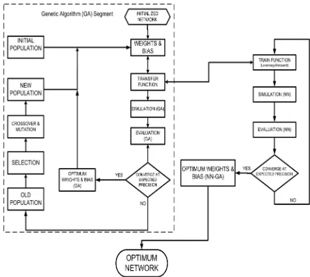
4. METHODOLOGY
The general procedure that was followed in
building the NN model is given in Figure 2.
The data made available for the producing
reservoir contained:
The Oil rate (BOPD)
Gas Produced (MscfD)
Water Production Rate (BOPD)
Among these data made available, the oil rate and gas produced were chosen as target and input variable respectively.
4.1 Neural Network Procedure
The Neural Network toolbox version 8.2 of Matlab 2014a was used to build the NARX network using back-propagation algorithm with the Levenberg-Marquardt training algorithm for the training procedure.
Fig. 2: Flowchart for NN modelling
The following steps were used in building this neural network:
Step 1: Specify Input and Targets; as stated earlier the Oil Rate was specified as target for the NARX network and the Gas produced was specified as the exogenous input.
Step 2: Determine Significant Correlations,
the input and target data are first normalized using Z-score normalization (In this method, data are changed so that their mean and variance are 0 and 1, respectively. The transformation function used for this method is:
= − ;
ℎ ℎ ℎ .
Cross-correlation of the input and target as well as autocorrelation of the target are used to determine the significant lags for the dataset
feedback delays are gotten from the significant auto-correlations of the target data.
Step 3: Determine the minimum number of hidden nodes that will give the best result and avoid over-fitting of the network. The minimum number is gotten by evaluating the network through multiple trials and the number of hidden nodes that give regression coefficient R2> 0.99, a NN of 10 hidden nodes would suffice
Step 4: Design open loop NARX net utilizing Mean Square Error (MSE) as the error estimation technique for performance criteria. A MSE target of 0.01is chosen.
Step 5: Now, the output feedback loop is closed and tested so that predictions can eventually be extended beyond the time of the known target. The MSE for the closed loop is also evaluated as the performance criteria.
4.2 Genetic Algorithm procedure
Step 1: Obtain the weight and bias vector of the closed loop NARX net which would be optimized by the Genetic algorithm.
Step 2: The optimization of the weight and bias vector is done with the aim of minimizing the MSE. Step 3: The optimized weight and bias vector is set as the weight and bias vector of the closed loop NARXnet.
The optimized NARXnet is then used for prediction of future time steps.
5. RESULTS AND DISCUSSION
Figure 3 gives shows the relationship between the target and input data over 1500 time steps (i.e. data points).
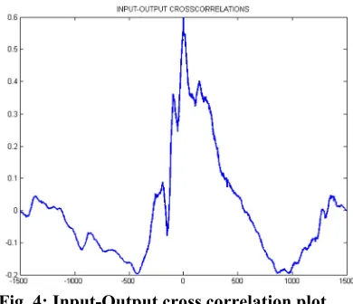
Figure 4 shows the significant lags as peaks of the input-output cross correlation plot, these are then used to determine the input delay.
Fig. 3. Relationship between input and output data.
Fig. 4: Input-Output cross correlation plot.
Figure 5(a) and 5(b) give the schematic representation of the open loop and close loop respectively.
(a)
(b)
Fig. 5(a) open loop schematic of neural network 5(b) closed loop schematic of neural network.
A comparison of the real data and the NN-GA model is given in Figure 6.
Fig. 6: Comparison of NN-GA Model with Real Data
It can be seen from figure 6 that the NN-GA model does well in predicting 500 time steps ahead after being trained with data of 1000 time steps.
6. CONCLUSION
The newly developed NN-GA model for predicting oil production from deepwater reservoirs was found to be accurate and better than the existing DCA technique. The advantage of NN-GA forecasting models is that prediction allows local variation instead of smooth curve projection as when DCA pattern is used. The use of both static and dynamic data extends the predictive capabilities of the ANN model from simple TS forecasting to spatial prediction. Preliminary clustering could be a good means to increase the precision of the forecasting. The case study comes from a single oilfield, nevertheless, the obtained conclusions may be applied to other deepwater reservoirs under pressure maintenance schemes. Further study is necessary to investigate the robustness of the proposed method and to establish data-driven NN-GA based reservoir models as a practical, cost-effective and robust tool for oilfield production management.
REFERENCES
1] Nikravesh, "Soft computing for intelligent reservoir D. Tamhane, P. Wong, F. Aminzadeh and M. characterization," in Proceedings of the SPE Asia Pacific Conference on Integrated Modelling for Asset
Management, Yokohama, 2000.
2]
W. Weiss, R. Balch and B. Stubbs, "How artificial intelligence methods can forecast oil production," in SPE/DOE Improved Oil Recovery
Symposium, Tulsa, Oklahoma, 2002.
3]
I. Batyrshin and L. Sheremetov, "Perception based approach to time series data mining," J. Appl.
Soft Comput, vol. 8, no. 3, p. 1211–1221, 2008.
4]
K. Li and R. Horne, "A decline curve analysis model based on fluid flow mechanisms," in SPE Western Regional/AAPG Pacific Section Joint
Meeting, Long Beach, CA, 2003.
5]
A. El-Banbi and R. Wattenbarger, "Analysis of commingled tight gas reservoirs," in SPE Annual
Technical Conference and Exhibition, Denver,
Colorado, 1996.
6]
A. P. Engelbrecht, Computational Intelligence: An Introduction, West Sussex: John Wiley & Sons Ltd, 2007.
7]
M. T. Hagan, H. B. Demuth and M. Beal, Neural Network Design, Boston: PWS Publishing Company, 1996.
8]
A. Sozen, E. Arcakilioglu and M. Ozalp, "Investigation of Thermodynamic Properties of Refrigerant/Absorbent Couples Using Artificial Neural Networks," Chemical Engineering and Processing, vol. 43, no. 10, pp. 1253-1264, 2004.
9]
S. Mohaghegh, M. Richardson and S. Ameri, "Use of intelligent systems in reservoir characterization via synthetic magnetic resonance logs," J. Pet. Sci. Eng, vol. 29, no. 1, p. 189–204, 2001.
10]
F. Aminzadeh, J. Barhen, C. Glover and N. Toomarian, "Reservoir Parameter estimation using a hybrid neural network," Comput. Geosci., vol. 26, no. 1, p. 869–875, 2000.
11]
A. Al-Kaabi and W. Lee, "Using artificial neural networks to identify the well test interpretation model," SPE Format. Eval. , vol. 8, no. 1, p. 233–240, 1993.
12]
C. Maschio, C. de Carvalho and D. Schiozer, "A new methodology to reduce uncertainties in reservoir simulation models using observed data and sampling techniques," J. Pet. Sci. Eng., vol. 72, no. 1, p. 110– 119, 2010.
13]
W. Habiballah, R. Startzman and M. Barrufet, "Use of neural networks for prediction of vapor/liquid equilibrium K-values for light-hydrocarbon mixtures," SPE Reservoir Eng., vol. 11, no. 1, p. 121–126, 1996.
14]
S. Al-Fattah and R. Startzman, "Predicting natural gas production using artificial neural network," in SPE Hydrocarbon Economics and Evaluation Symposium, Dallas, Texas, 2001..
15]
N. Bose and L. P. Bose, Neural Network
Fundamentals with Graphs, Algorithms and
Applications, 2nd ed., Boston: McGraw-Hill, 1996.
16]
M. de Souto, A. Yamazaki and T. Ludernir, "Optimization of neural networ kweights and architecture for odor recognition using simulated annealing," in 2002 International Joint Conference on Neural Networks 1, 2002.
17]
N. García-Pedrajas, C. Hervás-Martínez and J. Mu˜ noz-Perez, "A cooperative coevolutionary model for evolving artificial neural networks," in IEEE Transactions on Neural Networks 14, 2003.
18]