Path Planning and Obstacle Avoidance for Boe Bot Mobile Robot-

The Detection of Disease by Statistic Test of Analyze of Variance

Kaouther. El kourd1_{, Amer El kourd}2 1_{Electronic institute, Biskra} University Biskra

Algeria

2_{Department of computer} Islamic University Gaza Palestine

[email protected], [email protected]

ABSTRACT: From this article we used “application the analyses of variance”, Anova technique, which equal to mean

squares dividing by the mean squares of error, then applied the statistic study on the pathological image. After that, compeer the result obtained with student technique. The logicial applied is Matlab7.0 to extract the lesion by two way: distribution of Gaussian curve (hypothesis test of ho) and directly on the pathologique image.

Keywords: Regression, Fitted, Anova, Student

Received: 22 November 2012, Revised 29 December 2012, Accepted 2 January 2013

© 2013 DLINE. All rights reserved

1. Introduction

Analysis of variance became widely known after being included in Fisher’s 1925 book Statistical Methods for Research Workers. In statistics, analysis of variance (ANOVA) is a collection of statistical models, and their associated procedures, in which the observed variance in a particular variable is partitioned into componentsattributable to different sources of variation. In its simplest form, ANOVA provides a statistical test of whether or not the means of several groups are all equal, and therefore generalizes t-test to more than two groups. Doing multiple two-sample t-tests would result in an increased chance of committing an error. For this reason, ANOVAs are useful in comparing two, three, or more means. [1]

As problematic what’s the main of ANOVA technique? and what’s it’s performance if we compeer it for example with Student one?

2. Distribution & probability

2.1 Central aim of statistical tests

- H₁: statistically significant difference between sample & population (or between samples)

For example the distribution of events in a population for P (value | H₀) < 0.05.See figure (1)

Figure 1. Distribution of events for p < 0.05 [2]

σ = n n

i =

∑

(x_i −µ)2

µ = _n n

i =

∑

µ : is Population mean

3. Variance

Instead of thinking about the group means, we can instead think about variances. Recall sample variance (equation (3)):

s2 = n −1 n

i =

∑

(x_i −x)2

F = Variance 1/Variance 2

Model s 2

Error s 2 F = F: is ANOVA (ANALYSIS OF VARIANCE)

Total variance = model variance(S² model) or between groups) + error variance(S²E or within groups). [1] [2]

3. Correlation and Regression

Here we ask questions:

1) Is there a relationship between x and y?

Answer: yes if we applied the relation of covariance where it’s relation is:

(1)

(2)

(3)

(4) Wl

cov (x, y) =

n −1 n

i =

∑

(x_i − x) (y_i −y)

2) What is the strength of this relationship?

Answer: Pearson’s role said: [1] [2]

- Covariance does not really tell us anything but we can measure the standardises the covariance value, and Divides the covariance by the multiplied standard deviations of X and Y: [1]

=

(n −1) n

i =

∑

(x_i −x) (y_i −y) s_x s_y

r_xy =cov (x, y)

s_x s_y Where:

s_x s_y: Standard deviations

3) Can we describe this relationship and use it to predict y from x?

Answer: yes by using regressing then Fitting a line using the Least Squares solution.

3.1 Regression

Description about the relationship between two variables where one is dependent and the other is independent.

3.2 Fitted Regression Line

The true regression line corresponding to equation (1.a) is usually never known. However, the regression line can be estimated by estimating the coefficients β₁ and β₀ for an observed data set. [2]

E (Y) = β₀ + β₁ x

The actual values of y, (which are observed as yield from the chemical process from time to time and are random in nature), are assumed to be the sum of the mean value, E(Y), and a random error term, e: The actual values of y, (which are observed as yield from the chemical process from time to time and are random in nature), are assumed to be the sum of the mean value, E(Y), and a random error term, e: equation (1.b). [1] [2].

Y = E(Y ) + ∈

= β0 + β1 x + ∈

The estimates, β₁ and β₀, are calculated using least squares. The estimated regression line, obtained using the values of, β₁ and

β0, is called the fitted line. The least square estimates, β1 and β0, are obtained using the following equations: [1]

β1− =

n

i

∑

(x_i −x)2 n

∑

∑

y_ix_i

y_i x_i

⎝ ⎛ ⎝ ⎛ ⎞ ⎠ ⎞ ⎠ n − n

∑

β0− = y − β1 x

^ ^

Where y is the mean of all the observed values and x is the mean of all values of the predictor variable at which the observations were taken y is calculated using and is calculated using y =_⎝⎛ ⎞1_n⎠∗

∑

1 n

i=1

∑

∗ n ⎝ ⎛ ⎞ ⎠ x =

Once β₁ and β₀ are known, the fitted regression line can be written as:

(5) (6) (1.a) (1.b) (2) (3)

i ₌1 i =1

y = β^₀ + β^₁ x

where y is the fitted or estimated value based on the fitted regression model. It is an estimate of the mean value, E(Y). The fitted value, y_t , for a given value of the predictor variable, x_i, may be different from the corresponding observed value, y_i. The difference between the two values is called the residual, e_i:

∼ ∼

e_i = y_i− y^_i

To calculate the Statistic F_o , it must pass by the six titles: [2] [3] [4] [5] [6] [7]

3.2.1 Total Sum of Squares (SS_T)

On simple linear regression that the total sum of squares, SS_T , is obtained using the following equation: n

i =

∑

(y_i −y)2

SS_T− n

i=

∑

y_i2 n

i=

∑

y_i ⎝ ⎛ ⎞ ⎠ 2 n − −

The total sum of squares in matrix notation is:

SS_T= y’y − 1 y’Jy n

⎝ ⎛ ⎞

⎠

y’ [I −

= _⎝⎛ ⎞_n1_⎠J ] y

Where y is the vector of observed values, I is the identity matrix of order n; & J represents an n ×n square matrix of ones,

3.2. 2 Model Sum of Squares (SS_R)

Similarly, the model sum of squares or the regression sum of squares, SS_R, can be obtained in

n

i =

∑

y_i2 SS_R=

∑

⎝ ⎛ ⎞ ⎠ 2 n −

= y’ y − 1 y’Jy n

⎝ ⎛ ⎞

⎠

= y’ [ H − ^

J ] y

1 n ⎝ ⎛ ^ ⎞ ⎠

matrix notation as:

Where H is the hat matrix and is calculated using

H = X (X ’X)−1 X’

3.2.3 Error Sum of Squares

The error sum of squares or the residual sum of squares, SS_E, is obtained in the matrix notation from the vector of residuals, e, as:

SS_E = SS_T− SS_R

^ ^

= ( y − y )’( y − y ) = y’ ( I − H ) y

3.2.4 Mean Squares (MS_T)

Mean squares are obtained by dividing the sum of squares with their associated degrees of freedom. The number of degrees of freedom associated with the total sum of squares, SS_T , is (n −1) since there are n observations in all, but one degree of freedom is lost in the calculation of the sample mean y. The total mean square is:−

SS_T n −1 MS_T=

(4) (5) (6) (7) (8) (9) (10) (11) (12)

i ₌1

3.2.5 Regression mean square (MS_R)

The number of degrees of freedom associated with the regression sum of squares, SS_R, is k. There are (k + 1) degrees of freedom associated with a regression model with (k + 1) coefficients, β₀, β₁, β₂...β_k

However, one degree of freedom is lost because the deviations, (y_t− y) , are subjected to the constraints that they must sum to zero.

SS_R k MS_R=

The number of degrees of freedom associated with the error sum of squares is: n − (k + 1), as there are n observations in all, but (k + 1) degrees of freedom are lost in obtaining the estimates of β₀, β₁, β₂...β_k to calculate the predicted values, y_i. The error mean square is:[2] [3] [4] [5] [6] [7]

∼

SS_E n − (k + 1) MS_E =

The error mean square, MS_E, is an estimate of the variance, σ 2, of the random error terms, e_i.

3.2.6 Mean square error (MS_E)

Is estimate variance (σ ∼2) of random error e_i. see (equation 15 )

σ 2 _{= MS}

E ^

3.2.7 Calculation of the Statistic F_o

Once the mean squares MS_R and MS_E are known, the statistic to test the significance of regression can be calculated as follows: [2]

F_o= MS_E MS_R

4. Algorithm

1) It must converted MRI image IRM by (Dicom, Mrirco, SPM…) logigial to form (jpg.png, nii, img, hdr……..) for authorize the programmation with matlab.

2) choose a sample of image.

3) Analyse the sample -Analyze the data which is the protocol - Estimate the linear regression with parameters estimates (image x). - Extract the error between y & y estimate.

- Application the analyses of variance ‘ANOVA’ . 4) Conception & results .

5) Comparison between Student & Anova.

5. Program execution

5.1 Analysis of data (the protocol radiologic)

Our protocol is for a patient aged 15 years; who is present in clinical context of late stature and puberty with pituitary dysfunction. The patient is made by an MRI scan with injection of contrast medium. The machine is used radiologist type “SIEMENS”, and with the field B = 1.5 Tesla. The sequences performed T1-weighted and T2.

MRI appearance of a tumor of the median line developed at the expense of the floor of the third ventricle and the left sidewall responsible for a moderate hydrocephalus by compression phenomenon of holes monro.

(13)

(14)

(15)

(16) ~

The regression mean square is:

∑

n

This aspect is mentioned first craniopharyngioma. Galiale tumor diagnosis remains in the range.

Gonalgiques disorders are due to the tumor development at the expense of the hypothalamic region.

Figure 1 present an image normal (left) & pathologique one (right).

Figure 1. left. Normal image; right : Pathologique image

The figure (2) display the error (e) for one vector with length n = 200: see equation (5): e = y − y Where: y is the vector, & y is data estimate.

Y is with Blue color; y is with Red color & error is with blue star.

~

^

^

Figure 2. Presentation error e, y & Y

5.2 Calculate de Fcal: See equation (16) & figure (3) F- cal = MS_R/ MS_E

Where:

MS_R: The within-groups variation. MS_E: the between-groups.

Figure 3. Presentation de F-cal (point blue ), MS_R (red) color & MS_E (blue color)

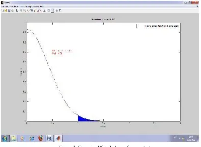
5.3 Distribution Gaussian (figure 4)

From table of test (fisher & student for α = 0.01) we have . * Degree of liberty: ddl: v = n −1= 200 −1 = 199. * F − tab = 1.

* Hypothesis ho will be :

If F− cal ≤ F− tab ⇒ f − test with (anova) Îaccept H_j.

If F−cal > F− tab ⇒ test F− test reject H_o.

⎧

⎨

⎩

5.4 Surface 50 × 50

For surface 50 × 50 with probability alpha = 0.01); figure 1 present pathologique image, to see clearly the lesion; we have on it translate the figure1 to binary to extract with precise the place of lesion with anova technique (color white). See figure (2). In figure 3 the curve display the error of number of samples: (10 to 35), the length more then 35 or less then 10 becomes the error near the zeros. In this matrix; Fisher table (ftab) = 1.85, so all results from fisher calculate (fcal = fo) superior then this value will be reject (c.a.d ho : reject), & all results inferior then 1.85 will be accept (ho : accept). Figure 5 present the result but with student technique; where here there isn’t any detection of lesion in t-test (student)).

5.5 Surface 100 × 100

Figure 4. Gaussian Distribution of anova-test

Figure 5.1. Pathologic image Figure 5.2. Detection of lesion with anova Figure 5.3. Pathologic image

Figure 6. Nomber of sample Figure 7. Anova ftab 0 20 40 60

2

0 -2

-4

-6

-8

0 1 2 3 0.8

0.6

0.

4.2

0

ho zone accept h1, r

Reject if mean > 1.84 Prob = 0.01

Error

Figure 8.1. Pathologic image Figure 8.2. Detection of lesion with anova Figure 8.3. Pathologic image

Figure 9. Nomber of sample _{Figure 10. Anova ftab}

Figure 11.1. Pathologic image Figure 11.2. Detection of lesion with anova Figure 11.3. Pathologic image with student

Figure 12. Nomber of sample Figure 13. Anova ftab

5.6 Surface 200 × 200

0 50 100 5

0 -5

-10

-15

-20

0 1 2 3 0.8

0.6

0.

4.2

0

ho zone accept h1, r

Reject if mean > 1.65 Prob = 0.01

Error _Density

0 50 100 150 200 0 1 2 3 ho zone accept h1, r

Reject if mean > 1.00 Prob = 0.01

1 0.8

0.6

0.4

0.2

0 20

0

-20

-40

-60

6. Conclusion

From these article we can distinct:

- Our study is applied for comparison between two models (normal image & pathological one) for medical image & (new model and old one) in the other specialty as: biologic, architect, medicament….ect.

- Anova techniques is used for small surface but student is used for small & middle surface - The result with Anova is more precise in front of ttest.

We propose using as perspective the technique of anova but for regression non linear.

References

[1] http://en.wikipedia.org/w/index.php?title = Factorial_ANOVA&redirect = no, 12/6/2012 at 15:00. [2] http://www.weibull.com/DOEWeb/introduction.ht;1 2/6/2012, 15-45.

[3] Research Methods I, ANOVA and Multiple Regression,

[4] UFR SPSE-Master, Université Paris X – Nanterre, PMP EF 205, Méthodes Statistiques pour l’analyse de données en psychologie. Chapitre 5. Comparaison deplusieursmoyennespourdes échantillonsindépendants (ANOVA), 2008-2009. [5] Viviane Kostrubiec. Les comparaisons multiples: entre mythe et réalité, Laboratoire Adaptations Perceptivo-Motrices et Apprentissage (EA 3191), Université Paul Sabatier–Toulouse III.

[6] Jon Roiser, Predrag Petrovic. (2006). t-tests, ANOVA and regression, February 1st.