Recursive Identification of Hammerstein Systems with Polynomial Function Approximation

(1)

http://www.sciencepublishinggroup.com/j/ijmfs doi: 10.11648/j.ijmfs.20170306.12

ISSN: 2575-4939 (Print); ISSN: 2575-4947 (Online)

Research/Technical Note

Recursive Identification of Hammerstein Systems with

Polynomial Function Approximation

Wang Jian-hong

1

, Tang De-zhi

2

, Jiang Hong

1

, Tang Xiao-jun

1 1

School of Electronic Engineering and Automation, Jiangxi University of Science and Technology, Ganzhou, China 2

School of Electrical and Information Engineering, Anhui University of Technology, Ma-an-shan, China

Email address:

[email protected] (Tang Xiao-jun)

To cite this article:

Wang Jian-hong, Tang De-zhi, Jiang Hong, Tang Xiao-jun. Recursive Identification of Hammerstein Systems with Polynomial Function Approximation. International Journal of Management and Fuzzy Systems. Vol. 3, No. 6, 2017, pp.87-94. doi: 10.11648/j.ijmfs.20170306.12 Received: September 25, 2017; Accepted: October 27, 2017; Published: November 20, 2017

Abstract:

Nonlinear system identification is considered, where the nonlinear static function was approximated by a number of polynomial functions. It is based on a piecewise-linear Hammerstein model, which is linear in the parameters. The identification procedure is divided into two steps. Firstly we adopt the extended stochastic gradient algorithm to identify some unknown parameters. Secondly using singular value decomposition (SVD), we propose a new method to identify other parameters. The basic idea is to replace un-measurable noise terms in the information vectors by their estimates, and to compute the noise estimates based on the obtained parameter estimates. The applicability of the approach is illustrated by a simulation.

Keywords:

Nonlinear System, Hammerstein Systems, Polynomial Functions Approximation, Recursive Identification, Singular Value Decomposition

1.

Introduction

Modeling, identification and prediction are three main ubiquitous phenomena in our daily lives. Through our ideas and senses, we collect information about the world, then we interpret, predict and react actions according to our perceptions. In natural science, lots of experiments or observations guide us to formulate laws of nature, which describe different aspects of the world and let us predict all sorts of things, like planet movements or weather forecast. Also in modern technology, modeling and identification have much benefit to offer us one description corresponding to the physical object. Everywhere and everything around us, there is a need for automatic control mechanisms such as in aero-planes, cars, chemical process plants, mobiles phones, heating of houses etc. However to be able to control a system, one needs to know at least something about how it behaviors and reacts to different actions taken on it. Hence we need a model of the system. A system can informally be defined as an entity which interacts with the rest of the world through more or less well defined input and output data. A model is then an approximate description of the system. An ideal model should

be simple, accurate and general. This approximate description of the system can be constructed by system identification strategy, as the goal of system identification is to build a mathematical model of a dynamic system based on some initial information about the system and the measurement data collected from the system. According to [1], the process of system identification consists of designing and conducting the identification experiment in order to collect the measurement data, selecting the structure of the model and specifying the parameters to be identified and eventually fitting the model parameters to the obtained data [2]. Finally the quality of the obtained model is evaluated through model validation process. Generally system identification is an iterative process and if the quality of the obtained model is not satisfactory, some or all of the listed phases can be repeated in order to obtain one satisfied model.

(2)

which has applications in many engineering problems and therefore, identification of Hammerstein models has been an active research topic for a long time. Existing methods in the literature can be roughly divided into six categories: the iterative method, the over-parameterization method, the stochastic method, the nonlinear least squares method, the separable least squares method and the blind method [4].

The Hammerstein model is a nonlinear system where a nonlinear block is followed by a linear dynamic block. The Hammerstein model has been widely used in many areas including nonlinear filtering, actuator saturations, audio-visual processes. There exists a large number of papers on the topic of the Hammerstein model identification. Reference [5] considered an extended stochastic gradient identification algorithm for Hammerstein-Wiener ARMAX systems. To improve the identification accuracy, an extended stochastic gradient algorithm with a forgetting factor is given. Reference [6] proposed three methods of separating the parameter estimates. The three methods are the averaged

method, permutation and combination method and singular value method. Reference [7] considered two identification algorithms, an iterative gradient and a recursive stochastic gradient based, for a Hammerstein nonlinear ARMAX model.

2. Problem Formulation

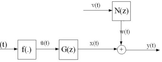
In this paper we focus on the identification of Hammerstein model which consists of a nonlinear memory-less element followed by a linear dynamical system [8]. The true output

( )

x t and the inner variable u t

( )

are immeasurable, u t

( )

is the system input, y t

( )

is the measurement of x t

( )

but is corrupted by the disturbance w t

( )

, the output of N z

( )

driven by an additive white noise v t

( )

with zero mean,

( )

G z is the transfer function of the linear part in the model,

( )

N z is the transfer function of the noise model [10].

Figure 1. The discrete time SISO Hammerstein system.

Assume that the linear dynamical block in Figure 1 is described by an ARMAX model, which has the

( ) ( )

( )

( ) ( )

( )

( ) ( )

( )

( ) ( )

( )

( ) ( )

y t x t w t B z x t G z u t u t

A z D z w t N z v t v t

A z

= +

= =

(1)

Here A z

( ) ( )

,B z and D z

( )

are polynomials in the shift operatorz−1_z y t−1

( ) ( )

=y t−1_ with

( )

1 2

1

1 d

d n n

n n

A z a z a z a z B z b z b z b z D z d z d z d z

− − −

−

− −

= + + +

= + +

= + + +

⋯

(2)

Notice that in the characterization of the Hammerstein model, f u

( )

and G z

( )

are actually not unique. Any pair

( ) ( )

(

af u G z, a

)

for some nonzero and finite constant

a

would produce identical input and output measurements. In other others, any identification scheme can not distinguish between

(

af u G z

( ) ( )

, a

)

and

(

f u G z

( ) ( )

,

)

. Therefore to

get an unique parameterization, one of the gains of f u

( )

and

( )

G z has to be fixed. There are several ways to normalize the gains.

A nonlinear static function can be approximated by a number of basis functions, connected to each other and forming a piecewise-linear function.

( )

T

u t =F u iC₍₃₎

where C is a vector of parameters representing values cjof the piecewise-linear function u t

( )

in knots.

( )

0 1 _{1 1}

T

j m _m

C c c c c

+ ×

 

=_ ⋯ ⋯ _ ₍₄₎

The knots are joints of line segments defined in terms of input signal

u

.

( )

0 1 _{1 1}

T

j m _m

u u u u u

+ ×

 

=_ ⋯ ⋯ _ ₍₅₎

satisfying

0 1 j j 1 m

u < < <u ⋯ u <u ₊ < <⋯ u

(3)

( )

0

( )

1

( )

₍ _{1 1}₎

T

j m _m

F u F u F u F u F u + ×

 

=_ ⋯ ⋯ _

Element of the vectorF u

( )

are defined as follows:

( )

0 m i j j i i i j u u F u u

u u = ≠ − = −

∏

substituting into equation (3), then the nonlinear part in the Hammerstein model is in the following form:

( )

0

m

j j j

u t f u u c f u =

= =

∑

(6)

with

( )

0 m i j j i i i j u u f u u u = ≠ − = −

∏

It can be easily seen that:

( )

1

0 j i ij

if i j f u

if i j

δ  =

= =

≠

 (7)

( )

j j

j

f u c

u

= (8)

Therefore the plant (1) can also be represented by the following model:

( ) ( )

( ) ( ) ( ) ( )

( )

0 0 m j j j m i j j i i i j

A z y t B z u t D z v t

u t f u u c f u

u u f u u u = = ≠ = + = = − = −

∑

∏

(9)

A regressive form can be derived as follows:

( ) ( ) ( ) ( ) ( ) ( ) ( ) ( ) ( )

1 0

( ) ( )

n m

i j j

i j

A z y t B z u t D z v t b u t i c f u t i D z v t

= =

= + =

∑

−

∑

− +

From the last equality, we can easily get the following recursive equation:

( ) ( ) ( ) ( ) ( )

1 1 0 1

( ) ( )

d

n

n n m

i i j j i

i i j i

y t a y t i b u t i c f u t i d v t i v i

= = = =

= −

∑

− +

∑

−

∑

− +

∑

− +

( ) ( ) ( ) ( ) ( )

1 1 0 1

( ) ( )

d

n

n n m

i ij j i

i i j i

y t a y t i µu t i f u t i d v t i v i

= = = =

= −

∑

− +

∑∑

− − +

∑

− +

where

1 , 0,1

ij b ci j i n j m

µ = = ⋯ = ⋯ ₍₁₀₎

Define the parameter vector θ and information vector

( )

t

φ as

( )

(

)

0 0 0 1 1 , n n d m a t v t

R t R

v t n d ϕ µ µ θ φ µ     _ _   _ _   _ ₋ _ = ∈ =_ _∈   _ _   __ ₋ __     ⋮

⋮ (11)

(

)

0 2 d

n = m+ n+n

1 2 n n a a a R a       =_ _∈     ⋮ , 10 20 0 0 n n R µ µ µ µ       =_ _∈     ⋮ 11 21 1 1 n n R µ µ µ µ       =_ _∈     ⋮ .. 1 2 m m n m nm R µ µ µ µ       =_ _∈     ⋮ 1 2 _d d n n d d d R d       =_ _∈       ⋮

( )

( ) 0 2 1 a m n m t t

t t R

t ϕ ϕ ϕ ϕ ϕ +         =_ _∈       ⋮

( )

(

)

(

)

1 2 _n a y t y t t R

y t n

ϕ ₋ ₋    − −   =_ _∈   − −    

⋮ (12)

( )

(

( )

)

(

)

(

)

(

)

(

)

1 1 2 2 , 0,1 j j n j j

u t f u t

t R j m

u t n f u t n ϕ  ₋ ₋     ₋ ₋  = ∈ =     − −     ⋯ ⋮

Then we have

( ) ( )

T

( )

y t =φ t θ+v t

Notice that ϕ

( )

t in φ

( )

t is available but

( )

( 1, 2 _d)

v t i i− = ⋯n _in φ

( )

_t _{are unavailable. Let}

θ

_ˆ

denotes the estimate ofθ. Since v t

( )

is a white noise with zero mean, then

( ) ( )

ˆ

ˆ T

(4)

It is the best output prediction. Consider the quadratic output prediction error criterion

( )

( ) ( )

2 2

1 1

ˆ _ˆ ˆ

t t

T

i i

J θ y i y i y i φ t θ

= =

 

=

∑

_ − _ =

∑

__ − __ (14)

The quadratic error function in (14) is one of the most common cost functions in the identification literature [9]. Many well-known Hammerstein model identification methods belong to this class and the differences lie only in the formulation of the information vectorφ

( )

t . Let

( )

1 1

,

1 ₁

T T

T

t y t

y t t

Y t t

y

φ φ

φ

 

 

−  − 

 

=_ _ Φ = 

 

  _ _

⋮ ⋮

(15)

Hence

( )

2

ˆ ˆT ˆ ˆ

J θ =_Y t − Φ t θ_{ } Y t − Φ t θ_= Y t − Φ t θ

Provided that Φ

( )

t is persistently exciting, minimizing

( )

ˆ

J θ gives the least-squares estimate:

( ) ( )

1

( ) ( )

ˆ T _t _t T _{t Y t}

θ

_{= Φ} _Φ − _Φ

  (16)

However a difficulty arises because of v t

( )

−i , Φ

( )

t in the expression on the right-hand side of (16) contains unknown noise terms v t

( )

−i i( =1, 2⋯n_d) _{, so it is} impossible to compute the estimate

θ

ˆ by (16), our approach is based on the iterative identification principle [10]. Let

1, 2

k= ⋯the unknown variables v t

( )

−i are replaced by their corresponding estimate vˆ_k

( )

t−i at iterationk , and φ

( )

t

are replaced by φˆ

( )

k [11]. Let

θ

ˆ_k be the iterative solution ofθ. Thus the estimate of v t

( )

is given by

( ) ( )

ˆ 1

( )

ˆ 1

ˆ_k _k _k

v t− =i y t− −i φ ₋ t−i θ ₋ (17)

( )

( ) ( )

(

)

0

ˆ 1

ˆ ˆ

k n

k

k d

t v t

t R

v t n

ϕ φ

   

−   =_ _∈

  −    

⋮

(18)

( )

ˆ

ˆ ₁

T k T k k

T k

t t t

φ φ

φ

 

 

 ₋ 

Φ = 

 

 

⋮

(19)

Based on (16) and replace Φ

( )

t byΦk

( )

t , the iterative solution

θ

ˆ_k of θmay be computed by:

( ) ( )

1

( ) ( )

ˆ T T _, _{1, 2}

k k t k t k t Y t k

θ

_{= Φ} _Φ − _Φ ₌

  ⋯ (20)

To initialize the algorithm, we take

θ

ˆ₀ =0or some small real vector, e.g.

0 6 0

ˆ ₁₀

n

I

θ ₌ − _with

0 n

I being an n₀

-dimensional column vector, whose elements are 1. As θ comes in linearly, algorithm (20) turns out to be adequate parameterization to get estimates of the parameters a_i,µ_ijand

i

d , using the iterative least squares algorithm.

3.

Basic Formulations for Plant Model

Identification

From estimates θˆ

( )

t ofθ, one has to get estimates

( )

b cˆ ˆ_i, _j of

( )

b c_i, _j fori=1⋯n j, =0,1⋯m_{. We will first construct a}

procedure to go back from µij's to b si' andc si' . Then relations to get

( )

b cˆ ˆ_i, _j from µij will be established.

Observe that (10) can be rewritten as follows:

10 1 1

0 1

m

n m n

b

M c c c

b

µ µ

   

   

=_ _=_ __ _

   

   

⋯

⋮ ⋮ ⋮ ⋮ ⋯

⋯

(21)

Notice that since Mis a rank-1 matrix, b s_i' andc s_i' can not be determined uniquely from µ_ij's , unless extra conditions are imposed on b s_i' and c s_i' . Uniqueness of the solution of (21) can be achieved by imposing the following couple of conditions:

2

1

1 n

i i

b =

=

∑

and ρ

(

b1⋯bn

)

>0 (22)

where ρ

(

b1⋯bn

)

denotes the first component of the vector

1

T n

b b

 

 ⋯  _{that satisfies:}

[

]

(

1

)

1

sup

n j

j n

b b b

ρ

≤ ≤ = ⋯

i.e the first component with a great absolute value.

Based on the above observations [11], a procedure is designed using singular value decomposition (SVD) [10].

Proposition 2.1. let M∈Rn m× +( )1 be any rank-1 real matrix. Then its SVD decomposition has the following form:

1 0 0

0 0 0

M

σ

 

 

= Γ_ _Σ

 

 

⋯

⋮ ⋮ ⋮

⋯

(23)

(5)

nonzero singular value of M . Furthermore M can be uniquely decomposed as follows:

[

]

1

0 1 m

n

b

M c c c

b     =_{ }    

⋮ ⋯ ₍₂₄₎

with

[

]

( ) [

]

[

]

1 1 1 0 0 0 0 T T n _T

b b sign r

σ

Γ = Γ ⋯ ⋯ ⋯ (25)

[

0 1

]

( )

[

1 0 0

] [

1 0 0

]

T T

m

c c ⋯ c =sign r Γσ ⋯ × ⋯ Σ

where

[

]

(

10 0

)

r=ρ Γ σ ⋯

The vector _b₁ ⋯ b_n_T_{thus obtained is the only solution}

of (23) that satisfies:

2 1 1 n i i b = =

∑

and ρ

(

b1⋯bn

)

>0

Estimates

( )

b cˆ ˆ_i, _j of

( )

b c_i, _j can be recovered fromµ_ij's. Following closely proposition 2.1[12], one first considers the matrix:

( )

10 1 0 ˆ ˆ ˆ ˆ ˆ m n nm t t M t t t µ µ µ µ     =      ⋯ ⋮ ⋮ ⋮ ⋯ (26)

Proposition 2.2: let the singular values decomposition of

( )

ˆ

M t be written as follows:

( )

1 2 0 0 0 ˆ 0 0

0 0 n

t t

M t t t

t σ σ σ      

= Γ _ _Σ

      ⋯ ⋮ ⋱ ⋯

Then proposition2.1 suggests the following estimates for the parameters

(

b c_i, _i

)

( )

( ) ( )

1 1 1 ˆ 0 0 0 0 ˆ T T n b t t t sign r t

t t b t σ σ     Γ   _ _ =  

  _Γ _ _

    ⋯ ⋮ ⋯ (27) ( ) ( ) ( ) ( )

( )

( ) ( ) [ ] ( ) 0 1 1 ˆ ˆ

0 0 1 0 0

ˆ

T

m

c t c t

sign r t t t t

c t

σ

   

 ₌ _Γ _ _ _× _Σ           ⋯ ⋯ ⋮ (28)

( )

(

( ) ( )

1 0 0

)

T

r t =ρ Γ t _σ t ⋯ _ (29) The estimates thus obtained are the only ones that satisfy the conditions

( )

(

)

2 1 1 1

ˆ ˆ ₀

n

i i

n

b t

b t b t

ρ

=

  _>

 

∑

⋯

Notice that the singular values σ2

( )

t ⋯σn

( )

t have not been accounted for in the rules (27), (28) and (29). It has no effect when theµij's converge to their true values, because the rank of matrix M tˆ

( )

converges to 1. This is made precisely in the next proposition.

Proposition 2.3: let

{ }

M tˆ

( )

be the real matrix sequence defined by (26). Let _b tˆ1

( )

⋯ bˆn

( )

t _ and

( )

0

ˆ ˆ_m

c t c t

 

 ⋯  be the vectors obtained from M tˆ

( )

according to the rules (27), (28) and (29). If the µ_ij's

converge to their true values µij , then the estimates

( )

(

ˆ _,_ˆ

)

j i

b t c t will converge to their true values

( )

b c_i, _j .

4.

Recursive Identification Algorithm

In this section, we derive a recursive identification algorithm which can be on-line implemented. We rewrite the equation.

( ) ( )

T

( )

y t =φ t θ+v t (30) Equation.(27) is a pseudo-linear regression identification model for the Hammerstein system. Note that ϕ

( )

t in φ

( )

t

is available but v t

( )

−i , i=1, 2⋯n_d_inφ

( )

_t _{are unavailable.}

LetE denote the expectation operator, θˆ

( )

t the estimate of

θ at timet, x =tr xx_ T_ the norm of the matrix

x

. Since

( )

v t is a white noise, forming a quadratic cost function

( )

( ) ( )

2 J θ =E__ y t −φ θt __

minimizing J

( )

θ leads to the following stochastic gradient algorithm of estimating θ

( ) ( ) ( )

( ) ( ) ( ) ( )

ˆ ˆ ₁ t T ˆ ₁

t t y t t t

r t φ

θ ₌θ _{− +}  ₋φ θ ₋ 

 

  (31)

( ) ( )

( )

2

( )

1 , 0 1

(6)

However the algorithm in (31) and (32) is impossible to realize because the information vector φ

( )

t on the right-hand side contains unknown noise termsv t

(

−k

)

. The solution is to replace the unknown variables v t

( )

−i with their corresponding estimatesv tˆ

(

−k

)

, and further define:

( )

( ) ( )

(

)

ˆ _ˆ ₁ _ˆ T

d

t t v t v t n

φ ₌_ϕ ₋ ⋯ ₋ _ ₍₃₃₎

From (33), we have

( )

( ) ( )

T

v t =y t −φ t θ

replacing φ

( )

t and θ in the above equation with φˆ

( )

t and

( )

ˆ _t

θ , the estimated residual can be computed by

( )

( ) ( ) ( )

ˆ ˆ

ˆ T

v t = y t −φ t θ t (34) replacing φ

( )

t in (31) and (32) withφˆ

( )

t , we can obtain the extended stochastic gradient [ ESG] identification algorithm of estimating θ

( ) ( ) ( )

ˆ

( ) ( ) ( ) ( )

ˆ ˆ ₁ t ˆ T ˆ ₁

t t y t t t

r t

φ

θ

₌

θ

_{− +}  ₋

φ

θ

₋ 

 

 

( ) ( )

2

ˆ

1 , 0 1

r t =r t− + φ t r = (35)

( )

(

)

ˆ 1

ˆ

ˆ _d

t v t t

v t n

ϕ φ

 

 

−

 

=_ _

 

−

 

 

⋮

( )

0

ˆ ˆ ˆ

ˆ ˆ

m

a t t

t

d t µ θ

µ

       

=_ _

       

⋮ ₍₃₆₎

To initialize this ESG algorithm θˆ 0

( )

is generally taken to be some small real vector, e.g.

0 6 0

ˆ ₁₀

n

I

θ ₌ − _with

0 n

I being an n₀-dimensional column vector whose elements are 1.

The ESG algorithm has low computation, but its convergence is relatively slow. In order to improve the tracking performance of the ESG algorithm, we introduce a forgetting factor λ in the ESG algorithm to get the ESG algorithm with a forgetting factor, which is referred to the EFG algorithm.

( ) ( ) ( )

( ) ( ) ( ) ( )

( )

( ) ( )

2

ˆ

ˆ ˆ ₁ ˆ ˆ ₁

ˆ

1 , 0 1, 0 1

T t

t t y t t t

r t

r t r t t r

φ

θ θ φ θ

λ φ λ

 

= − + __ − − __

= − + = < <

(37)

whenλ=1, the EFG algorithm reduces to the ESG algorithm.

5.

Simulation

A simulation is given to demonstrate the effectiveness of the proposed algorithms.

Consider the following system:

( ) ( )

A z y t =B z u t +D z v t

( )

1 2 1 2

1 2

1 1 1.60 0.80

A z = +a z− +a z− = − z− + z−

( )

1 2 1 2

1 2 0.80 0.60

B z =b z− +b z− = z− + z−

where

2 2

0.80 +0.60 =1

( )

1 1

1

1 1 0.64

D z = +d z− = − z−

( )

0 0 1 1 2 2

0 1 2

0.20 0.40 0.60

u t u c f u c f u c f u u f u f u f u

 

=  + + 

 

=  + + 

where

( )

2

0

i j

j i i i j

u u F u u

u u

= ≠

− =

−

∏

[

1.60, 0.80, 0.16, 0.24, 0.32, 0.24, 0.48, 0.36, 0.61

]

T

θ= − −

( )

{ }

u t is taken as a persistent excitation signal sequence with zero mean and unit variance σ_u2 =1.002, and

{ }

v t

( )

as a white noise sequence with zero mean and constant variance

2

v

(7)

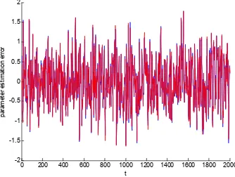
Solid line: the ESG algorithm; dots: the EFG algorithm. (λ=0.98)

Figure 2. The parameter estimation error δ versust.

Figure 3. The parameter estimation error δ versus t of the EFG algorithm.(λ=0.90).

6. Conclusion

We have considered system identification based on Hammerstein model, where the nonlinear element is defined by a piecewise-linear function. We have designed an identification scheme that determines precisely the unknown nonlinear parameters

( )

b ci, j i=1⋯n j, =0,1⋯m and

those of the linear transfer function. An iterative algorithm based on replacing un-measurable noise variables by their estimates are derived for Hammerstein nonlinear models.

Acknowledgements

This work was supported by the Grants from the National Science Foundation of China (no. 61563022), the Jiangxi

0 200 400 600 800 1000 1200 1400 1600 1800 2000

-2 -1.5 -1 -0.5 0 0.5 1 1.5

t

p

a

ra

m

e

te

r

e

s

ti

m

a

ti

o

n

e

rr

o

r

0 200 400 600 800 1000 1200 1400 1600 1800 2000

10-5 10-4 10-3 10-2 10-1 100

t

E

rr

o

r

v

a

lu

(8)

Provincial National Science Foundation (no. 20142BAB206020, no. GJJ150889), and the National Science Foundation of the Colleges and University in Anhui Provincial (no.KJ2016A094).

References

[1] Anna Hagenblad, Lennart Ljung, Adrian Wills. Maximum likelihood identification of Wiener models[J]. Automatica, 2008.44(11):2697-2705.

[2] Lennart Ljung. System Identification: Theory for the user [M], Prentice-Hall, Upper Saddle River, 1999.

[3] Martin Enqvist, Lennart Ljung. Linear approximations of nonlinear FIR systems for separable input processes. Automatica [J], 2005. 41(3):459-473.

[4] J. J. Bussgang. Cross correlate on functions of amplitude-distorted Gaussian signals. Technical Report Technical report 216, MIT Laboratory of Electronics, 1952. [5] Bai E-W. Frequency domain identification of Hammerstein

models[J]. IEEE transactions on automatic control. 2003. 48(4):530-541.

[6] Bai E-W. A random least-trimmed-squares identification algorithm [J]. Automatica. 2003. 39(9): 1651-1659.

[7] Bai E-W. Identification of linear systems with hard input nonlinearities of known structure [J]. Automatica, 2002. 38(5): 853-860.

[8] Lennart Ljung. Estimating linear time invariant models of non-linear time-varying system [J]. European Journal of Control, 2001. 7 (2):203-219.

[9] R. Pintelon, J. Schoukens. Fast approximation identification of nonlinear systems [J]. Automatica, 2003. 39(7):1267-1273. [10] Ding F, Tongwen Chen. Identification of Hammerstein

nonlinear ARMAX systems [J]. Automatica, 2005. 41 (9):1479-1489.

[11] Ding F, Tongwen Chen. Performance analysis of multi-innovation gradient type identification methods [J]. Automatica, 2007. 43(1):1-14.