Scalable Computing: Practice and Experience
Volume 15, Number 1, pp. 33–48. http://www.scpe.org
ISSN 1895-1767 c
2014 SCPE
ADAPTIVE MULTI-GRID METHODS FOR PARALLEL CFD APPLICATIONS∗
J´ER ˆOME FRISCH, RALF-PETER MUNDANI, AND ERNST RANK
Abstract. Computational fluid dynamic (CFD) computations are memory and time intensive and need to be executed in
parallel for larger computational domains. In order to produce physical accurate solutions, adaptive grid setups have to be chosen as the memory and computing time would otherwise be too high, and results would not be obtained in a reasonable amount of time. This paper describes the usage of a multi-grid based approach for solving the pressure Poisson equation, arising during every time step of the Navier-Stokes equations. It will then highlight an analysis of errors introduced due to an adaptive setup of the domain, and show performance measurements for uniform and adaptive grid setups. Last but not least, a CFD benchmark example based on the von K´arm´an vortex street will be presented, and the results will be discussed.
Key words: parallel computation, adaptive data structure, multi-grid like solver, computational fluid dynamics, Poisson
equation, message passing paradigm
AMS subject classifications. 65Y05, 65G99, 65M55, 35J05, 76D05
48
1. Introduction. Computational fluid dynamics (CDF) simulations are time intensive and require a lot of computational resources. Hence, every optimisation or algorithmic speed-up has huge benefits for expensive long running scenarios in terms of energy efficiency and CPU costs. Moreover, design parameters regarding domain setup or solver settings also prove to have a high impact on run times.
Uniform grids exhibit huge advantages due to very easy computations via stencil-based operations, they require no additional grid management, and are very easy to implement (cf. [5]). Thus, it is very cost efficient using structured uniform grids for computations. One disadvantage of such an approach is the required equidis-tant discretisation of the entire domain, which is not always necessary depending on the geometry settings. For an engineering based air-flow simulation of an indoor airspace for example, regions have to be computed very fine around obstacles but do not necessarily need to have the same resolution at regions far away from these obstacles. Thus, a geometry based, adaptively refined grid has huge advantages in terms of reducing unnecessary refinements.
Adaptive grids are already quite well studied in literature. There exist several possibilities of generating adaptive grid refinements. One possibility is the stepwise approximation with regular grids, such as the approach described in this paper or from Manhart and Wengle [13]. Another possibility which will not be regarded for this code would be the overlapping of two different grids of different resolution, so called Chimera grids, as studied by Hadˇzi´c [11]. Furthermore, boundary adapted non-orthogonal grids could be used. All methods have advantages and disadvantages listed in detail in [5]. The authors chose to use the approximation with hierarchical block-structured grids, as they fit quite well to the used data structure.
The main CFD implementation is based on an incompressible Newtonian fluid flow simulation governed by the Navier-Stokes equations. The spatial discretisation is realised by a finite-volume scheme and for the temporal discretisation currently an explicit forward Euler method enhanced by the Adams-Bashforth method of 2nd order is applied. Further details are given in section 6.
A Poisson equation for the pressure term has to be solved in every step of the fluid solver, hence this step needs to be analysed in detail in order to speed up the solution process. This paper will describe a multi-grid based approach for solving the pressure Poisson equation which is deeply integrated in the data structure itself, and takes advantage of the internal exchange functions and similar concepts of the two approaches. Further details can be found in section 4.
The paper quickly outlines the applied hierarchical data structure for block-structured, orthogonal Cartesian grids and presents additions to compute with an adaptively refined grid structure. For a fair parallel efficiency, a load distribution has to be performed in order to balance the computational effort to the various machines. A detailed analysis concerning errors generated by an adaptive refinement is presented and a performance overview is given. Last but not least, an adaptively refined von K´arm´an vortex street is computed as test example, which is according to Hirsch [12] a simple geometry which generates a quite complex flow.
∗Chair for Computation in Engineering, Technische Universit¨at M¨unchen, 80290 Munich, Germany ([email protected]).
This paper is based on the conference publication [8], and was extended by including a section on the multi-grid based solver concept, as well as further performance measurements and an enhanced error evaluation.
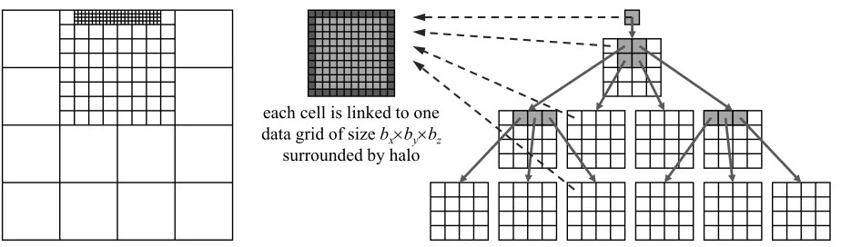
2. Data Structure Layout. The data structure is based on block-structured, non-overlapping, regular, orthogonal Cartesian grids organised in a hierarchical management grid as depicted in figure 2.1. Two main components form up the system: the management grids on the one hand and the data grids on the other hand. The management grids are ordered according to a hierarchical organisation structure in a tree-like fashion starting from a root grid (also called top grid, cf. figure 2.1 on the right hand side). They contain logical information such as parentage or children links. One management grid can have up to 73 management grid
children, although the refinement in each dimension can be selected separately.
A special case is the so called octree data structure, if the child refinement is set to 2 in every direction, giving 23management grid children per parent grid. Furthermore, the refinement of the root (rtx, rty, rtz) can be chosen
differently than that of any subsequently refined grid (rs
x, rsy, rzs), in order to allow for a useful discretisation of
e. g. a channel. A refinement of ri = 1 can be chosen in order to impose a non-refinement in a given axis i,
which can be useful for a pseudo-2D computation. The refinement levels impose certain limits on the accuracy of the solution in an adaptive area, and thus, studies about accuracy will be carried out in section 5 of this paper in order to quantify this approximation.
each cell is linked to one data grid of size bxubyubz
surrounded by halo
Fig. 2.1.Logical data structure layout in tree form (on right-hand side) and in overlayed grid form (on left-hand side). Each
logical grid holds a pointer to a data grid containing the actual data surrounded by a halo of ghost cells (mid of picture). (Picture based on [9])
The second main part of the data layout is formed by the data grids depicted in the middle of figure 2.1. Each management grid is linked to exactly one data grid, which will hold the actual computational data of all internal fields, such as velocities, pressure, temperature, etc. The size of a data grid is fixed to (bx, by, bz) for
all grids, with the restriction, that bi has to be dividable without remainder by ritand rsi for all iin order to
avoid non-conforming grid boundaries.
This data structure setup enables a strict separation of computation and communication phases. From the user’s point of view, a new kernel can be implemented on a regular Cartesian grid. Everything else which has to do with adaptivity, interpolation, or data exchange is outsourced to communication functions which are called by one single call from within the kernel. Thus, an expert in his area of research can easily implement a new computational kernel without being an expert in parallel computing or computer science.
As last step, all the ghost cells of the grids have to be filled which have not been touched in the previous horizontal communication phase. Therefore, data stored in the current ghost cells of the parent grids are used to interpolate values in the ghost cells of the child grids. Further information about the communication procedures or the grid setup can be found in [6, 9].
It should be mentioned that unlike in similar concepts, the intermediate grids are not discarded during the refinement process. Hence, all grids are kept in memory, even if refined children are available. The actual computation however, will be carried out only on the ‘leaf’ (i. e. non-refined) grids. This concept has some considerable advantages. For one, the applied solver for the Poisson problem introduced in section 4 is using the parent grids for its internal solving procedures.
A second advantage is that if a very fast computational response is necessary, such as in the case of a computational steering approach (cf. [19]), e. g., a maximal computation depth can be imposed, where higher refinements will be disregarded, and a coarser but faster computation can be performed on the exact same data structure.
As third advantage, a visualising technique for reducing the amount of transferred data can be applied easily, such as described in [16], called sliding-window approach. Here, a certain window of interest as well as a maximal bandwidth can be fixed. A special server-sided collector decides which data on which level will be sent to a client-sided visualisation application. Thus, interactive data visualisation can be managed at run-time with constant bandwidth requirements for data exchange.
3. Parallel Data Distribution and Load Balancing. For a parallel computation, a good data distri-bution is inevitable in order to minimise communication over the network. The following section will describe how such a distribution can be achieved by using space-filling curves.
3.1. Neighbourhood Server Concept. For a load distribution or redistribution, two different strategies can be applied: a global view or a local view strategy. In the local view strategy, a diffusion process as proposed by Cybenko [4] can be applied. No information about the global system is necessary, and work is only distributed to the direct neighbours. This process has to be repeated a certain amount of steps, until an overall balanced distribution has been reached. On the other hand, a global view can do the distribution in one single step by having global knowledge of the problem. Unfortunately, the process having the global view typically becomes a bottle neck with an increasing amount of processes in the system.
Nevertheless, due to its better characteristics the authors chose to implement a global view concept. A dedicated server, the so called ‘neighbourhood server’, keeps track of all management grids without having any actual data of the grids themselves. Using this concept, rebalancing and grid migrations are easily possible without a lot of overhead. Possible bottle-neck simulations are avoided by having multiple servers running concurrently and serving different processes. Details of the synchronisation procedures can be found in [7].
3.2. Load Balancing using Space-Filling Curves. The neighbourhood server contains all management grids and can compute the best possible data distribution according to a certain given strategy. Possible distribution strategies should ensure a good data locality, i. e. keeping neighbouring grids as close as possible, and thus, minimising communication efforts. Space-filling curves deliver a good distribution for such purposes (cf. [1]).
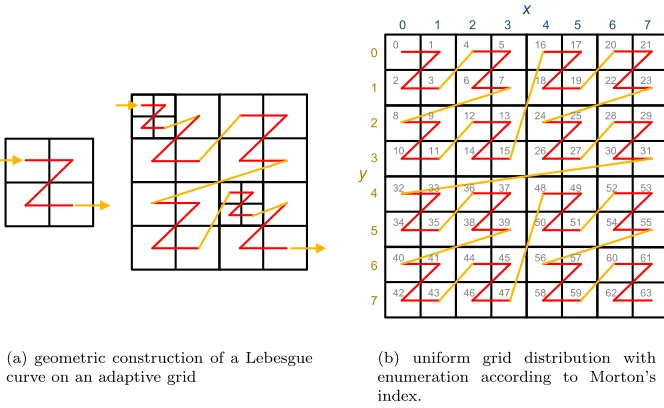
Of all the possible space filling curves (SFC), such as Hilbert, Lebesgue, Sierpi´nski, or Peano, among many others, the authors chose to use the Lebesgue curve depicted in Figure 3.1. The main reason for this choice is the very simple computation of the position of a given cell in the grid. The geometric construction of the curve can be seen in Figure 3.1(a). On the left-hand side, the geometric primitive is shown. Each part in the grid can then be refined further by applying again the construction primitive (due to the form of the primitive, the curve is also referred to as ‘z-order curve’).
The hierarchical tree is traversed in a depth first approach, respecting on every level the geometric primitive of the construction, thus delivering the figure on the right-hand-side of figure 3.1(a). Contrary to other work (e. g. [20]), the parent grids are not omitted, but also pushed to the linearised list. Thus, the list of grids on the right-hand-side would have a size of 29, even if only 22 of them are currently visible. This linearised list is split into (nearly) equal parts and distributed by means of grid migration to different computing processes.
(a) geometric construction of a Lebesgue curve on an adaptive grid
0 1 2 3 4 5 6 7
0 1 2 3 4 5 6 7 y x 0 2 8 10 32 34 40 42 1 3 9 11 33 35 41 43 4 6 12 14 36 38 44 46 5 7 13 15 37 39 45 47 16 18 24 26 48 50 56 58 17 19 25 27 49 51 57 59 20 22 28 30 52 54 60 62 21 23 29 31 53 55 61 63
(b) uniform grid distribution with enumeration according to Morton’s index.
Fig. 3.1.Load balancing strategy by applying Lebesgue’s curve and Morton’s indexing.
compute the position in the grid using Morton’s index [15], which can be generated easily by bit-interleaving. As example, an 8×8 grid is depicted in Figure 3.1(b). By writing the desired coordinates in binary form and padding them to the largest multiple of two, one can generate the Morton index by interleaving each bit from y with each bit fromx. Conversion from binary into decimal form delivers then Morton’s index. As example, x= 5, y= 3 is written in binary formx= 101, y= 011. By bit-interleaving, one obtains 011011 which reads in decimal 27 and corresponds to the Morton index ofx, y. The same procedure works in 3D by usingx, y,and z coordinates.
4. Multi-Grid Like Solver Concept. As mentioned in the previous section, the solver concept is based on a multi-grid like approach for the pressure Poisson equation. The basics, describing the mathematical properties, convergence studies, etc can be found in [2, 18, 10]. Putting it into a nutshell, a multi-grid based approach can be described as follows:
Let’s suppose the Poisson equation A·u =f should be solved on a given grid discretisation Ωh with a
spacing ofh. First, a smoothing using a 2/3 damped Jacobi relaxation method is appliedα1 times, obtaining
an approximation to the solution vh on this grid. The residual rh =fh−Ah
·vh is computed and restricted
to a coarser grid using a restriction operator I2hh to serve as right-hand side f2h. On the coarser grid Ω2h, the
residual equationA2h·e2h =f2h is relaxed to obtain an approximation to the error e2h. Again, the residual
r2h=f2h−A2h
·e2his computed and restricted to an even coarser level using a restriction operatorI4h
2h.
This procedure is repeated until the coarsest levelLhas been reached, where the residual equation system
ALh·eLh=fLhis small enough to be solved directly. AftereLhis known, the error correction is prolongated to
the finer grids and added to the approximation of the solutionv. Assuming the error correctione4h is known,
then the approximation on level 2hcan be obtained bye2h=e2h+I2h
4h·e4h, whereI24hhdescribes the prolongation
operator. The error is then relaxed α2 times using the 2/3 damped Jacobi smoother, before the prolongation
to level his performed. In the end, the error correctioneh is added to the approximation of the solutionvh.
This procedure is called a v-cycle and is the simplest form of a multi-grid approach. This v-cycle has to be repeated until the norm of the residual is below a given tolerance, at which point the system is solved to the given accuracy.
meaning that no matrixAis explicitly assembled, but a stencil operator is used for iterating over the grid points in memory. As the data grid uses a collocated data arrangement, where all values are stored in the cell centre, the data for the multi-grid also needs to be interpreted as cell-centred. As consequence, coarsened points do not coincide with finer points.
The amount of levels and thus, implicitly the amount of grid coarsening is dictated by the data structure itself and by the approximation of the geometry which should be solved.
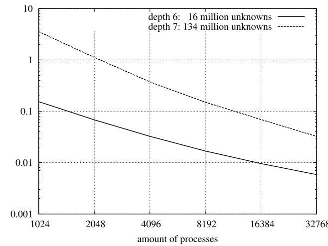
Figure 4.1 shows performance measurements on ‘Shaheen’, a 16-rack Blue Gene/P system having a total of 65536 compute cores at King Abdullah University of Science and Technology (KAUST) in the Kingdom of Saudi-Arabia1. Figure 4.1(a) shows the pure data exchange times for exchanging all ghost layers of 9 independent
variables for different problem sizes using up to 32768 processes. The curves show, that the communication time is decreasing while using more processes. Figure 4.1(b) shows strong scaling results for two different problem sizes for a 3D Laplace problem discretised uniformly up to a given depth. It can be seen, that a certain saturation is reached for a higher amount of processes. This happens earlier for the 16 million unknowns and starts later for the 134 million unknowns due to increased communication overhead and less work per process. The standard multi-grid algorithm uses a certain amount of smoothing steps α1 for the residual equation
and α2 for the error correction. These values are usually in a range of approximately 2–3. The multi-grid like
concept needs more smoothing steps in order to converge to the correct solution, especially when obstacles are present in the domain.
Following the ideas of [14], boundary conditions need to be handled on coarse grids in order to reproduce the effect they exhibit on the fine grids. Therefore, they need to be restricted in some way onto coarser grids. Dirichlet conditions have the highest priority, i. e. if one of the child cells has a Dirichlet boundary condition, the coarse cell will be marked as having a Dirichlet boundary condition. Neumann boundary conditions have a very low priority, and will only be restricted as Neumann conditions on the coarse grid if all child cells had Neumann boundary conditions. Otherwise, the coarse cell will be marked as fluid cell. As consequence, huge Dirichlet regions will appear in the coarsest grid representation, which can only be handled by a higher amount of smoothing towards the boundary regions.
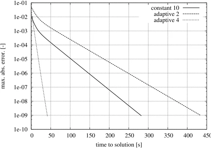
Figure 4.2 shows a plot of the error convergence for different smoothing strategies until a maximal error of 10−9 was reached. While applyingα
1 =α2= 10 on every level, 153 cycles were needed to converge (curve
‘constant 10’). A next approach is to adaptively changeαover different levels. On fine grids,αshould be small, as exchanging data is costly. On coarser grids however, αcan be increased as less data has to be exchanged, which produces less communication overhead. Hence, the plots named ‘adaptive’ use such a concept. ‘Adaptive 2’ starts with 2 smoothing steps on the finest level. In the next coarser level, 4 steps are used, then 8 and so on. This curve shows an even worse convergence than the constant 10. ‘Adaptive 4’ uses 4 smoothing steps to start on the finest level, then 8 on the next coarser, then 16 and so on. This curve shows exceptionally good convergence and needs only 27 cycles to converge to an error of 10−9 whereas ‘adaptive 2’ needed 477 cycles.
This study shows that attention has to be paid to the choice of settings for the solver, as small changes could generate a huge performance impact.
5. Performance and Accuracy Measurements of the Adaptive Data Structure. In order to evaluate the performance as well as the accuracy of the used data structures and its solvers, a Poisson equation will be solved for a simple test geometry. The use of the Poisson equation is realistic, as this equation has to be solved in every time step of a CFD simulation for evaluating the pressure-correction in order to obtain a divergence free velocity field of an incompressible fluid flow after each time step, and thus, ensuring the validity of the continuity equation.
5.1. Test Case Setup. The 3D test case geometry is composed out of a 1×1×1m block. The top-level as well as the subsequent refinement levels are set to bisection (rt
i = ris= 2 ∀i). The block size of the data
grids is set to bi = 12 in every direction. Dirichlet boundary conditions are imposed on all 6 walls. The west
and east wall in x-direction are set to 1.0 whereas all other walls are set to 0.0. The right-hand-side f of the Poisson equation ∆p=f is set to 0, thus describing actually a pure Laplace equation.
1
0.001 0.01 0.1 1 10
1024 2048 4096 8192 16384 32768
data interchange time [s]
amount of processes
depth 6: 16 million unknowns depth 7: 134 million unknowns
(a) Communication times for a total ghost cell exchange of 9 independent variables in seconds on ‘Shaheen’ for a 3D domain of fully refined grids with a refinement level (2,2,2) up to depth 6 or 7 and a data grid size of (4,4,4).
1 10 100 1000
1024 2048 4096 8192 16384 32768
time to solution [s]
amount of processes
depth 6: 16 million unknowns depth 7: 134 million unknowns
(b) ‘Shaheen’ strong scaling with different depths and block sizes of (4,4,4)
Fig. 4.1.Performance Measurements for different problem sizes for a 3D Laplace problem on an uniformly refined grid using
1e-10 1e-09 1e-08 1e-07 1e-06 1e-05 1e-04 1e-03 1e-02 1e-01
0 50 100 150 200 250 300 350 400 450
max. abs. error. [-]
time to solution [s]
constant 10 adaptive 2 adaptive 4
Fig. 4.2. Time to solution for different choices ofα1,2 computed on 1024 processes on ‘Shaheen’ for a 3D Laplace problem
on an uniformly refined grid in depth 6 using refinements (2,2,2) and block sizes (4,4,4).
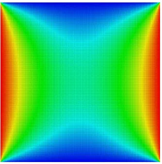
Figure 5.1 shows a 2D cut through the 3D test problem case (red meansp= 1.0, blue means p= 0.0). In the case of a uniform refinement, all grids were refined up to a certain depth. The amount of grid cells in the complete system can be computed for this example by
dmax
X
d=0
2d·s3 =
dmax
X
d=0
2d·123
.
In this case, the total amount of grid cells can be given as follows: depth 4 has approximately 8 million cells, depth 5 has 64.7 million cells, and depth 6 has 517.7 million cells. The cut shown in Figure 5.1(a) is depicted for depth 4 in order to better illustrate the grid refinement. The solution on level 6 is regarded as sufficiently fine and, thus, used as a reference solution.
According to the setting of the boundary conditions, the highest gradients are expected near the walls, thus in the case of an adaptive grid the refinement is increased closer to the boundaries by refining the bisected parts. Figure 5.1(c) shows a grid with a uniform refinement up to level 2 and two consecutive refinements towards the west and east walls. Figure 5.1(b) shows the results computed on that adaptive grid. Hence, such a grid is from now on called adaptive 2+2 ora2 + 2. Close to the west and east walls, the two setups have the same grid size, and are thus comparable.
5.2. Distribution Performance. In order to check the distribution for a real 3D problem, the distribu-tion and communicadistribu-tion patterns were analysed using the integrated performance monitoring tool IPM2. The
measurements were performed on ‘Shaheen’. Furthermore, some computations were done on the one-rack Blue Gene/P having in total 4096 compute cores at Universitatea de Vest din Timi¸soara (UVT) in Romania3.
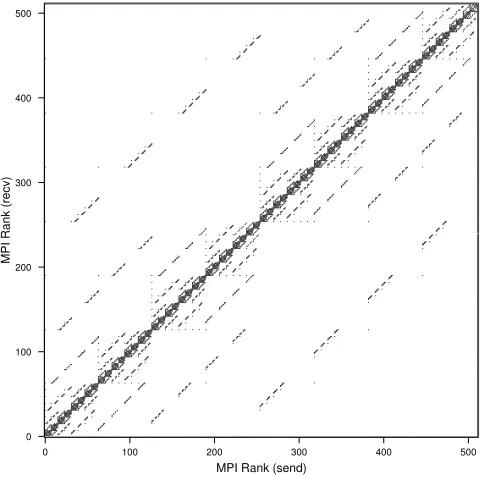
Figure 5.2 shows two distribution patterns for parallel computations using 512 processes performed on Shaheen. The communication pattern of theu4 refinement is depicted in Figure 5.2(a), the a2 + 2 refinement is shown in Figure 5.2(b).
2
Integrated Performance Monitoring (IPM):http://ipm-hpc.sourceforge.net
3
(a) Uniform Grid Distribution setup at depth 4 (u4)
(b) Adaptive Grid Distribution setup at depth 4 (a2 + 2)
(c) Adaptive Grid Distribution setup at depth 4 (a2 + 2) (grid only) and the cutline (in red) introduced in subsection 5.3
MPI Rank (send)
0 100 200 300 400 500
MPI Rank (recv)
0 100 200 300 400 500
(a) Communication Pattern Uniform setup up at depth 4
MPI Rank (send)
0 100 200 300 400 500
MPI Rank (recv)
0 100 200 300 400 500
(b) Communication Pattern Adaptive setup up at depth 4 (2+2)
Black markers depict a communication between the ranks on the x- and y-axis. In both patterns, the communication with the neighbourhood server residing on rank 511 is obvious and marked completely black, as each process gets its neighbouring information once from the server which will be cached until a change occurs. Otherwise, the main communication is focussed on a diagonal, indicating that only processes close to each other communicate with each other. Independent of the underlying network topology of the respective hardware, this shows that the average number of communication partners per process is small. In case of a non-locality preserving grid distribution, a much higher amount of communication partners could be seen in the communication diagram and would consequently slow down the communication in the system.
It can be observed, that the adaptive grid setup is not differing a lot from the uniform setup, which shows that the data distribution using the selected space filling curve is working as expected by preserving the locality of the data.
5.3. Accuracy Measurements. A first glance at the colour distribution of Figure 5.1 gives already a good hint, that the computations are not that far off and in the same order. To better quantify the error made by the adaptive approach, further treatment is necessary. In Figure 5.3, a quantification of the error is given.
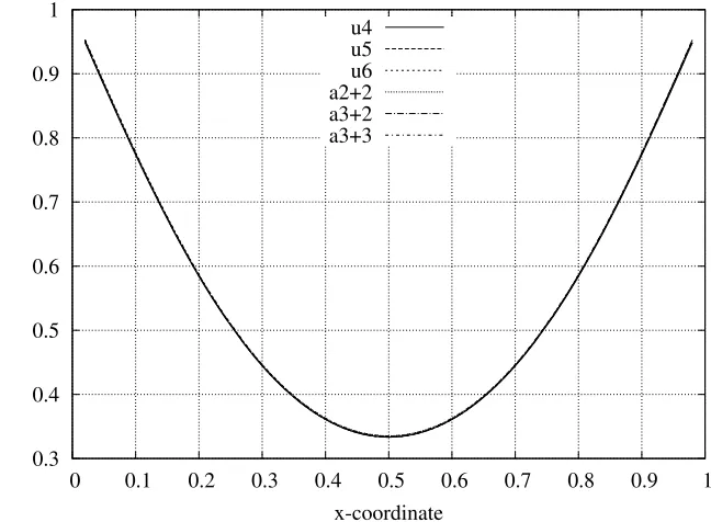
Figure 5.3(a) shows the value for the pressure in the complete domain for different simulation setups. The plot is shown over a cutline going inx-direction through the domain while maintainingy andz at 1/2. Thus, x= 0 represents the west wall andx= 1 represents the east wall having each Dirichlet boundary conditions of p= 1. On the other walls in the 3D domain, the boundary conditions are set top= 0. As solver, the multi-grid like solver from section 4 is used on the adaptive data structure. To be able to draw 1D results along a cutline, a trilinear interpolation is applied, for interpolating the values along the cutline out of the cell-centred values stored in the model.
In Figure 5.3(a) the general behaviour of the solution is similar. For better quantification, the relative error is plotted in Figure 5.3(b). As reference solution, a linear interpolation of the finest computation of a uniform distribution at depth 6 was used. The relative error is computed by the formula
erel= p−pref,u6 pref,u6
·100 [%] .
First of all, uniform grids at different levels were compared, namely level 4 and 5. The results show that the error is larger towards the boundaries than in the middle of the domain. This is due to the fact, that the larger cells cannot capture the higher gradients closer to the wall as good as the refined grids can. In the middle of the domain, where the gradients are small however, the approximation is quite good. Level 4 is worse than level 5, but nevertheless, the computational time and memory consumption are much better. On Sandstorm, the department for Computation in Engineering’s own cluster, with four nodes consisting each of two Intel Xeon E5-2690 processors with 8 cores each and a total of 768 GB of main memory, one node using 16 processes needed 6.8 seconds to compute the 8 million cells on level 4 and 98.5 seconds to compute the 64.7 million cells on level 5.
Furthermore, the error from the adaptive refinement with respect to the reference solution can be seen in Figure 5.3(b). Obviously the coarsest grid (a2 + 2) has the largest error. Towards the boundary,a2 + 2 shows the same error as u4 which is not remarkable, as the grids cells have the same size. Towards the middle, the error increases, as the grid is not fine enough to capture effects noticeable on the reference grids. A maximum error of approximately 0.6% can be observed for the a2 + 2 curve, which is with respect to all factors such as runtime and memory reduction quite acceptable.
Moreover, it can be noticed that the uniform grids never overestimate the solution of the reference grids, i. e. that the solution never ‘crosses’ through the reference solution. This is not the case with the adaptive refinement. Here, some solutions cross ‘through’ the reference solution (i. e. crossing the x-axis).
5.4. Scaling and Performance Measurements. Scaling and performance measurements for uniform grids using up to 32768 processes were already presented in section 4. The following section will provide a few comparative measurements to assess the performance impacts of the adaptive distribution. The measurements were performed on the UVT Blue Gene/P for the same 3D test case described above. The only difference is, that the block size of the data grids was set tobi= 4 instead of 12. Experience suggested that the Blue Gene/P
0.3 0.4 0.5 0.6 0.7 0.8 0.9 1
0 0.1 0.2 0.3 0.4 0.5 0.6 0.7 0.8 0.9 1
pressure
x-coordinate u4 u5 u6 a2+2 a3+2 a3+3
(a) Pressure distribution along the cutline
-0.6 -0.4 -0.2 0 0.2 0.4 0.6
0 0.1 0.2 0.3 0.4 0.5 0.6 0.7 0.8 0.9 1
relative error [%]
x-coordinate u4 - u6 u5 - u6 a2+2 - u6 a3+2 - u6 a3+3 - u6
(b) Relative error in % along the cutline
Fig. 5.3. Data along the cutline inx-direction through the domain aty=z= 0.5. The geometric position of the cutline is
0 0.1 0.2 0.3 0.4 0.5 0.6 0.7
0 200 400 600 800 1000
complete exchange time [s]
# grids per proc. adapt 2+4
adapt 2+5 unif 5 unif 6
(a) Exchange time in seconds plotted over the amounts of grids per process
0 20 40 60 80 100 120
0 200 400 600 800 1000
walltime to solution [s]
# grids per proc. adapt 2+4
adapt 2+5 unif 5 unif 6
(b) time to solution plotted over the amounts of grids per process
Fig. 5.4.Scaling and performance measurements on the UVT Blue Gene/P. A bisection to the given depth was chosen. The
Figure 5.4(a) shows scaling results for the pure exchange time in seconds of all the necessary variables for the fluid code (3 velocity values, a pressure value, a temperature value, etc). Figure 5.4(b) shows the wall time in seconds until a solution of the Poisson equation converged to an error below 10−9.
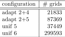
Thex-axis displays the amount of grids per process, in order to better compare the resulting times of the adaptive and uniform distributions. Computations were performed using up to 1024 processes. Table 5.1 shows the amount of grids in the different configurations.
Table 5.1
Amount of grids for different configurations used in the performance measurements
configuration # grids
adapt 2+4 21833
adapt 2+5 87369
unif 5 37449
unif 6 299593
It can be seen, that the performance of the exchange as well as the solution of the Poisson equation using the multi-grid-like approach is behaving well if less than 600 grids per process are used. On the other hand, a very similar behaviour of the adaptively refined grids can be observed. Hence, it can be concluded, that the adaptive refinements have no negative impact on the overall performance of the code. Contrary, a similar performance can be obtained with less computing power for simulating a domain with nearly the same accuracy but far less grids.
6. Adaptive CFD Example. The implemented CFD code for simulating an incompressible Newtonian fluid flow is currently based on the fractional step method proposed by Chorin [3]. In this approach, an explicit time stepping scheme is used. First, intermediate velocities are computed by omitting the pressure part in the Navier-Stokes equations. Then, using these intermediate velocities, the divergence of the momentum equation is computed leading to a Poisson equation for the pressure. After solving the Poisson equation, the obtained pressure correction is used to correct the intermediate velocity field leading to the velocities at the next time step.
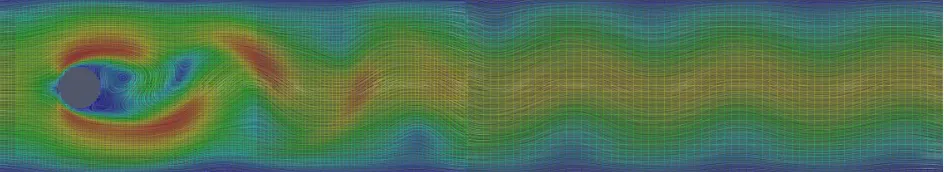
As engineering example of a non-steady-state fluid flow application, the von K´arm´an vortex street was computed according to the settings of the 2D-2 benchmark of Sch¨afer and Turek [17]. It is basically a channel flow with a cylinder as obstacle in the channel. After a certain simulation time, vortices start to shed from the disturbances downstream of the cylinder and will be transported out of the region.
Figure 6.1 shows the results of computations for different refinement levels using a Reynolds number of 100. For the a3 + 2 setting, the area consists of 405 adaptively organised grids in a hierarchy going up to depth 5 with an increased refinement around the area where the cylinder is located and the shedding of the vortices starts. a3 + 3 has a more refined resolution around the cylinder using 597 grids. In case the area would be uniformly refined up to level 5, the domain would contain 1365 grids and 5461 grids for level 6 respectively.
Using a normal desktop computer, a speed up of approximately 7.8 could be achieved by using the a3 + 3 version versus the fully refined u6 version (having around 9.1 times more grids), which corresponds also quite nice to the results of the scaling of the solution of the Poisson equation shown in Figure 5.4.
For the 2D-2 benchmark, the adaptive code delivered a Strouhal number (St =D·f /U¯, where D is the diameter of the obstacle,f is the frequency of the vortex shedding and ¯U is the mean input velocity as defined in [17]) of 0.290 which correlates very good with the experimental results ofSt= 0.287±0.003. Furthermore, the pressure difference ∆P between the front and the back of the cylinder delivered values between 2.40 and 2.48 depending on the state of the shedding which also corresponds quite well to the benchmark’s Table 4 in [17]. These results confirm that the fully adaptive CFD computation as it is currently implemented delivers reasonable physical results.
(a)a3 + 2 refinement
(b)a3 + 3 refinement
Fig. 6.1.Adaptively refined von K´arm´an vortex street according to the Sch¨afer-Turek benchmark 2D-2 atRe=100 (represented
by LIC (line integral convolution) overlaid with the grid refinement. The colour code represents the velocity magnitude. The current time of the two computations is different).
7. Conclusion and Outlook. In this paper, the authors presented a detailed study about an adaptive layout for a parallel distributed data structure capable of computing fluid flow simulations, as well as the main idea of a multi-grid based solver approach. The accuracy of the adaptive data structure as well as the introduced error was analysed and the influence on distribution and performance was evaluated. It could be shown, that introducing an adaptive layout does not have a negative influence on either performance or distribution, and the error is acceptable if compared to the massive gain in CPU time and memory consumption.
The solution process of the Poisson equation for the pressure correction could be considerably improved by applying a multi-grid-like solver on an adaptive domain. Future work includes further optimisation of the CFD code in order to increase the performance of long time consuming transient computations. Furthermore, the explicit time stepping scheme should be replaced at some point by an implicit scheme which allows larger time steps in the domain. Moreover, run-time adaptivity according to fluid criteria, such as maximal gradients of velocities, can be tackled and incorporated, which will improve the quality of the solution enormously.
Acknowledgments. This publication is partially based on work supported by Award No. UK-c0020, made by King Abdullah University of Science and Technology (KAUST). Furthermore, the authors would like to cordially thank for the support and usage of the Blue Gene/P at Universitatea de Vest din Timi¸soara (UVT) in Romania.
REFERENCES
[1] M. Bader,Space-Filling Curves - An Introduction with Applications in Scientific Computing, vol. 9 of Texts in Computational
Science and Engineering, Springer-Verlag, 2013.
[2] W. L. Briggs, V. E. Henson, and S. F. McCormick,A Multigrid Tutorial, Society for Industrial and Applied Mathematics,
Philadelphia, PA, USA, 2nd rev. ed., 2000.
Fig. 6.2. Adaptively refined von K´arm´an vortex street according to the Sch¨afer-Turek benchmark 3D-2Z atRe=20. The colour code represents the velocity magnitude.
[4] G. Cybenko,Dynamic load balancing for distributed memory multiprocessors, Journal of Parallel and Distributed Computing,
7 (1989), pp. 279–301.
[5] J. H. Ferziger and M. Peric,Computational Methods for Fluid Dynamics, Springer, 3rd, rev. ed ed., 2002.
[6] J. Frisch, R.-P. Mundani, and E. Rank,Communication schemes of a parallel fluid solver for multi-scale environmental
simulations, in Proc. of the 13th International Symposium on Symbolic and Numeric Algorithms for Scientific Computing (SYNASC), Timi¸soara, Romania, Sept. 26.-29. 2011, pp. 391–397.
[7] ,Resolving neighbourhood relations in a parallel fluid dynamic solver, in Proc. of the 11th International Symposium on Parallel and Distributed Computing, Los Alamitos, CA, USA, 2012, IEEE Computer Society, pp. 267–273.
[8] ,Adaptive distributed data structure management for parallel CFD applications, in Proc. of the 15th International Symposium on Symbolic and Numeric Algorithms for Scientific Computing (SYNASC), Timi¸soara, Romania, Sept. 23.-26. 2013, pp. 513–520.
[9] ,Parallel multi-grid like solver for the pressure Poisson equation in fluid flow applications, in Proceedings of the IADIS International Conference - Applied Computing, Fort Worth, Texas, USA, 2013, pp. 139–146.
[10] W. Hackbusch,Multi-Grid Methods and Applications, Volume 4 of Springer Series in Computational Mathematics, Springer,
2010.
[11] H. Hadˇzi´c,Development and Application of Finite Volume Method for the Computation of Flows Around Moving Bodies on
Unstructured, Overlapping Grids, PhD Thesis, Technische Universit¨at Hamburg-Harburg, 2005.
[12] C. Hirsch,Numerical Computation of Internal and External Flows, Volume 1, Butterworth–Heinemann, 2nd ed., 2007.
[13] M. Manhart and H. Wengle,Large-eddy simulation of turbulent boundary layer flow over a hemisphere, in first ERCOFTAC
Workshop on ‘Direct and Large-eddy Simulation’, Guildford, Mar. 27–30 1994, Kluwer Academic Publisher.
[14] A. McAdams, E. Sifakis, and J. Teran,A parallel multigrid Poisson solver for fluids simulation on large grids, in ACM
SIGGRAPH/Eurographics Symposium on Computer Animation (SCA), 2010.
[15] G. M. Morton,A computer oriented geodetic data base; and a new technique in file sequencing, tech. report, IBM Ltd.,
Ottawa, Canada, 1966.
[16] R.-P. Mundani, J. Frisch, and E. Rank,Towards interactive HPC: Sliding Window Data Transfer, in Proc. of the 3rd
Inter-national Conference on Parallel, Distributed, Grid and Cloud Computing for Engineering (ParEng2013), P´ecs, Hungary,
2013.
[17] M. Sch¨afer and S. Turek, Benchmark computations of laminar flow around cylinder, in Flow Simulation with
High-Performance Computers II, E. Hirschel, ed., vol. 52 of Notes on Numerical Fluid Mechanics, Vieweg, Jan. 1996, pp. 547– 566.
[18] U. Trottenberg, C. W. Oosterlee, and A. Sch¨uller,Multigrid, Academic Press, 2001.
[19] R. van Liere, J. D. Mulder, and J. J. van Wijk,Computational steering, Future Generation Computer Systems, 12 (1997),
[20] T. Weinzierl and M. Mehl,Peano – a traversal and storage scheme for octree-like adaptive cartesian multiscale grids, SIAM Journal on Scientific Computing, 33 (2011), pp. 2732–2760.
Edited by: Teodor Florin Forti¸s
Received: Feb 28, 2014