On the Localization Algorithm of Wireless Sensor Network and Its Application

(1)

On the Localization Algorithm of Wireless Sensor

Network and Its Application

https://doi.org/10.3991/ijoe.v13i03.6858

Honglei Jia

Jilin University, Changchun, China [email protected]

Jiaxin Zheng

Gang Wang *

Yulong Chen

Dongyan Huang Jilin University, Changchun, China

[email protected]

Hongfang Yuan Jilin University, Changchun, China

Abstract—This paper carries out in-depth and meticulous analysis of the DV-Hop localization algorithm for wireless sensor network. It improves the DV-Hop algorithm into a node localization algorithm based on one-hop range, and proposes the centroid particle swarm optimization localization algorithm based on RSSI by adding the RSSI and particle swarm optimization algorithm to the traditional centroid localization algorithm. Simulation experiment proves that the two algorithms have excellent effect.

Keywords—DV-Hoplocalization algorithm; WSN localization; one-hop; RSSI; particle swarm optimization algorithm.

1 Introduction

(2)

information processing and data operations [2-4]. However, thanks to the outstanding performance, it has enjoyed great popularity in the field of network communication. The network is capable of acquiring a gigantic amount of information from all as-pects. With the large number and various types of sensor nodes, it satisfies all kinds of information needs [5]. In the WSN, the independent wireless sensor nodes have lim-ited ability to detect, send and receive information. However, when multiple sensor nodes are combined into one, the WSN would have an increasingly stronger capabil-ity of information detection, transmission and reception[6]. In order to control the numerous sensor nodes, it is necessary to set up a special network protocol. With the protocol in place, it is possible to manage and control the data acquisition and pro-cessing of the nodes, and to carry out monitoring and information identification of all kinds of information within the radiation of the network, thereby fulfilling the corre-sponding monitoring purposes [7-8].

As is known to all, computer communication undergoes a significant change in computing model every 15 years [9]. The pattern applies to virtually every country in the world although it is based only on the experience of developed countries. Driven by computer communication technology, the human society is rapidly entering the Internet era[10]. The invention and extensive use of the Internet have already brought unprecedented changes to the economic, politics and social conditions of the world. As a result, almost all countries across the globe are stepping up the investment on information infrastructure [11-12]. Many new computer networks start to appear in the investment craze. Among them, the fast growing one is the WSN. The network is, in essence, an Internet of Things that links up sensors, water conservancy networks, power grid, road networks, communication networks, and pipe networks. At the dawn of the ear of the Internet of Things, the WSN is having an immense impact to people’s living and working environments [13]. With the further development and maturation of relevant technologies, it can be expected that the WSN would be deeply applied to every aspect of the social life.

2 The structure of WSN

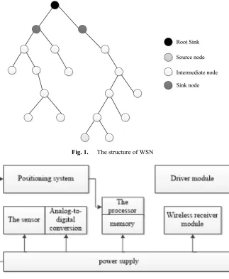
The main components of WSN are sensor nodes, sink nodes and management nodes. The network links up the user, the detection target, and the sensor nodes in an efficient manner, making it easier to detect the target [14].

Figure 1 illustrates the specific structure of the network. There are many sensor nodes in the monitoring area, which are combined in a certain way to synergically detect the target. After detecting the relevant information of the target object, the nodes pre-process the information and send the pre-processed information to the sink nodes. Then, the sink nodes send the received information to the control terminal. The user can communicate with the sink nodes through the computer network. Upon re-ceiving the monitoring request, the sink nodes send a command to the sensor nodes, asking the latter to transmit the acquired data to the sink nodes [15-16].

(3)

Intermediate node

Root Sink

Sink node

Source node

Fig. 1. The structure of WSN

Fig. 2. The hardware structure of WSN

3 The improved DV-Hop algorithm

3.1 The design of node structure

The structure of WSN must be carefully designed for it has a significant effect on the processing performance of the whole network [17]. In the traditional DV-Hop algorithm, the location information of the anchor node broadcast is in the format of

{id, xi, yi, Hopsi}, where the variables respectively represent the number, coordinates

(4)

In the improved algorithm, however, each node has its corresponding information structure. If the node is unknown, the corresponding information structure is {id, xi, yi,

Hopsi}. The only difference from the traditional format is the addition of the variable

Aid. The variable has multiple values. If the value is 0, the anchor node can be deter-mined as a level 1 anchor node, i.e. embedded in the system. If the value is 1, the anchor node can be regarded as a level 2 anchor node, which is transformed from a localized unknown node. If the value is 2, the anchor node should be categorized as a level 3 anchor node although it can also be converted from an unknown node. To minimize the localization error, researchers generally choose advanced nodes to lo-cate the unknown node. The format of the information on the unknown node contains two parts: the former part is the broadcast information, including the node number, coordinates, etc., and the latter part is the variable depicting how the unknown node used to receive and store the data packets from the anchor node. In short, the infor-mation should be expressed in the following format:{i, Ai, xi, yi, Hopsi}. The format contains the corresponding incident angle value, the coordinates of the node, and the variable of the information.

3.2 The localization of unknown node

(1) When all anchor nodes in the network are in the broadcast state, the anchor nodes send data packets on their location information to all the unknown nodes within their communication coverage. The data packets are in the format of {i, Ai, xi, yi,

Hopsid, Di}. id stands for the number assigned to an anchor node. Each node has a unique identification number. That is because the nodes in the network have no inher-ent order, making it possible to encode the inher-entire network in numbers. The id value is pre-set and should not be changed. The coordinates of the anchor node is obtained by GPS tools, which are highly accurate. The judgement should be make after the infor-mation sent by the anchor node reaches the unknown node. The value of Hopsid pro-vides the basis for judgement. If the value equals 1, save the received data packet; if it is not 1, discard the received data packet. As the nodes in WSN are not configured regularly, the one-hop range of an unknown node is not definite. In this case, as long as a packet of Hopsid=1 is received, the node is in the suspended state and no longer receives any more packet. During data reception, the unknown node also judges the Aid of the data packet and makes choices based on the priorities. If a data packet has a high priority and the corresponding Hopsid=1, it would be saved while the data pack-ets of low priority would be discarded. However, if the received data packet has a highly prioritized Aid, but the hop count is not 1, it would not be saved earlier than the data packets with Hopsid=1. The hop count is prioritized because the analysis in this paper is based on the localization algorithm within the one-hop range. The initial value of Aid is either 0 or 1. If it is 0, the corresponding node should be regarded as an unknown node, which cannot send data packets. Thus, if Aid is 0, the node can partic-ipate in the localization of other nodes.

(5)

within the one-hop range of the unknown node. With a determined anchor node, the RSSI algorithm can be used for the localization. The new RSSI localization algorithm satisfies strict requirements on localization and reaches higher levels of short distance measurement accuracy. The measured distance between the unknown node and the anchor nodeis generally noted as Di. The variable is usually initialized as 0. After determining the distance between the unknown node and the anchor node, the re-searcher should measure the incident angle between the two nodes. The measurement mainly relies on the AOA algorithm. To ensure the accuracy, the angle is normally measured in the counter-clockwise direction and the result is saved as i.

(3) After all the information is processed, the researcher should perform geometric calculation to get the coordinates of the unknown node.

cos

sin

pi i i i

x

D

y

D

!

= +

"#

$

₌

₊

#%

Obtaining the coordinates of the unknown node, the researcher needs to convert the node into an anchor node. Some of the parameter values in the packet are fixed, while the value of Aid would change. If the value is 1, it can be concluded that the reference anchor node used to localize this node is embedded in the system; if the value is 2, the reference anchor node should be deemed as a level 2 node. Hence, the value of Aid determines which type of anchor node the unknown node would be converted into. After conversion, change the hop count back to 0, save the coordinates of the corre-sponding node, and thereby obtain the data packet of the new anchor node.’

(4) After it is determined, the new anchor node would broadcast information to the unknown nodes within its own communication coverage and, at the same time, send the data packets it receives. Then, the researcher should convert the corresponding unknown node. In this way, all the qualified anchor nodes would be obtained. The localization would be complete when the entire network is traversed.

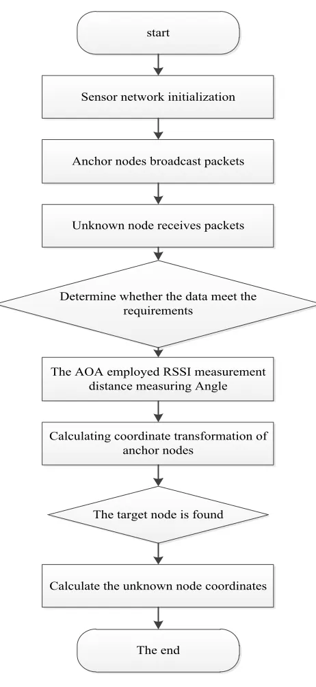
3.3 The flowchart of the improved algorithm

The function of the improved algorithm has also undergone great changes. See Figure 3 for the flowchart. The improved algorithm achieves very high network cov-erage by making use of the broadcast function of the original algorithm. The most striking feature of the algorithm is the addition of multiple new nodes, which dramati-cally expands the localization range.

4 Algorithm simulation and result analysis

(6)

algorithms. On this basis, the algorithm can be improved to get higher localization accuracy.

start

Sensor network initialization

Anchor nodes broadcast packets

Unknown node receives packets

Determine whether the data meet the requirements

The AOA employed RSSI measurement distance measuring Angle

Calculating coordinate transformation of anchor nodes

The target node is found

Calculate the unknown node coordinates

The end

(7)

5 10 15 20 25 30 35 40 6

7 8 9 10 11 12

The av

er

age pos

iti

on er

ro

r

The anchor node number DV-Hop changed algorithm

Fig. 4. Comparing the errors of different numbers of anchor nodes

(1) Taking different numbers of anchor nodes

Based on Figure 4, it can be seen that the two algorithms discussed in this paper have basically unchanged network parameters and the only difference between them lies in the changing values of the anchor node. In this figure, the number of anchor nodes falls between 5 and 40 and the step size is 5. If the total number of nodes in the network remains the same, the localization accuracy of both of the algorithms would rise in different degrees, resulting in lower error rate, as the number of anchor nodes increases. Nevertheless, on the whole, the improved algorithm is more powerful than the traditional one, featuring much better localization accuracy.

0.05 0.10 0.15 0.20 0.25 0.30 0.35 0.40 0.2

0.3 0.4 0.5 0.6

The av

er

age pos

iti

on er

ro

r

The anchor node proportion DV-Hop changed algorithm

(8)

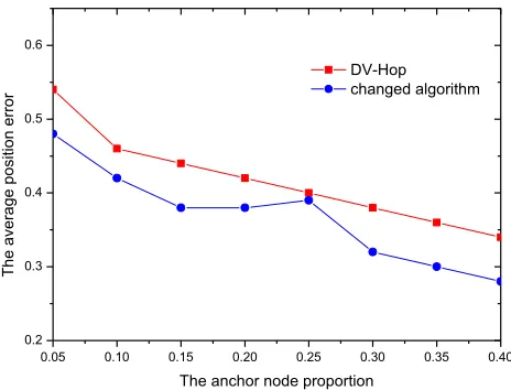
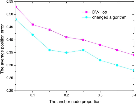
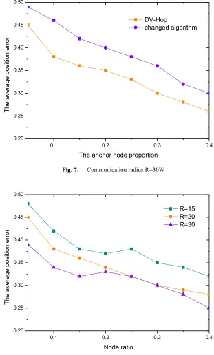
(2) Simulation of different communication radiuses

This section talks about the simulation carried within different communication ra-diuses. Figures 5, 6 & 7 display the simulation results at three different communica-tion radiuses: R=15m, 20m and 30m. In these figures, the x-axis stands for the ratio of the number of anchor nodes to the total number of network nodes, while the y-axis represents the average localization errors of the two algorithms. Comparing the three figures, the author discovers that the number of anchor nodes is closely related to the accuracy of the algorithms. With the increase of the number of the nodes, both algo-rithms have higher localization accuracies and lower error rates. Besides, the error of the improved algorithm decreases more significantly than that of the other algorithm. Further comparison indicates that, when the communication radius is 15m, the error of the improved algorithm is 2%-15% smaller than that of the traditional algorithm; when the communication radius is 20m, the error of the improved algorithm is 2%-7% smaller than that of the traditional algorithm; when the communication radius is further increased to 30m, the error of the improved algorithm is 2%-10% smaller than that of the traditional algorithm. The statistics reveal that the improved algorithm is much more accurate than the traditional one within short distances. See Figure 8 for the specific localization accuracy of the improved algorithm at different communica-tion radiuses. It is clearly described in the figure that there is a certain correlacommunica-tion between the communication radius and the localization error. As the communication radius increases, the algorithm has an increasing high accuracy and increasingly low error value. As a result, the communication error can be reduced by lengthening the communication radius.

0.1 0.2 0.3 0.4

0.20 0.25 0.30 0.35 0.40 0.45 0.50 0.55

The av

er

age pos

iti

on er

ro

r

The anchor node proportion DV-Hop

changed algorithm

(9)

0.1 0.2 0.3 0.4 0.20

0.25 0.30 0.35 0.40 0.45 0.50

The av

er

age pos

iti

on er

ro

r

The anchor node proportion DV-Hop

changed algorithm

Fig. 7. Communication radius R=30W

0.1 0.2 0.3 0.4

0.20 0.25 0.30 0.35 0.40 0.45 0.50

The av

er

age pos

iti

on er

ro

r

Node ratio

R=15 R=20 R=30

(10)

5 Conclusion

This paper mainly improves the traditional DV-Hop algorithm, and proposes a new node localization algorithm based on one-hop range. After that, the author carries out in-depth analysis of the principles and performance of the two algorithms and verifies the performance by simulation. To sum up, this paper mainly deals with the following issues:

(1) Through the analysis of the localization principle of the algorithm, the author holds that it is possible to measure the spacing between anchor node and unknown node via RSSI technology. In accordance with the requirements on specific distance localization, the author reaches the conclusion that the RSSI helps reduce the meas-urement error.

(2) The author introduces the AOA measurement technology. The technology im-proves the accuracy of weapon attack because it can easily determine the orientation of anchor node, and identify the incident angle between the two nodes.

(3) This paper mainly localizes the nodes by the mathematical method so that the data can be easily processed in a computer. In this way, the calculation error is re-duced without sacrificing the calculation speed.

(4) In the meantime, this paper uses anchor nodes to assist in localization. If an un-known node has been localized, it can be used to help with the localization of other unknown nodes. Since some nodes are far away from or beyond the measuring range of the anchor node, it is necessary to increase the number of anchor nodes to improve the coverage of the network, thereby fulfilling the monitoring purposes.

(5) The author selects the priority method to determine the appropriate anchor nodes, and transforms unknown nodes according to the existing anchor nodes. Be-sides, the author classifies the nodes into different levels, and chooses the most priori-tized anchor nodes to help with the localization.

(6) Finally, the author simulates the two algorithms, compares the measuring accu-racies and errors between the two, and provides the flowchart and complier language of the new algorithm.

6 Acknowledgment

Thanks very much for 12th _{Five Year National Science and Technology Support} Plan (Grant No.: 2014BAD06B03), the Science and Technology Development Pro-gram of Jilin Province (Grant No.: 20160441004SC). These financial supports are gratefully acknowledged.

7 References

(11)

[2]Li, J. Y., Wang, J. P. (2014). Wireless sensor network mobile agent routing based on the improved ant colony algorithm. Journal of Convergence Information Technology, 8(5), 585-592. https://doi.org/10.4028/www.scientific.net/amm.587-589.2339

[3]Aktouf, O. E. K., Parissis, I. (2012). SMART service for fault diagnosis in wireless sensor networks, Proceedings - 6th International Conference on Next Generation Mobile Appli-cations. 211-216.

[4]Lu, T. J., Wang, Y. (2014). Application of improved ant colony algorithm technology in development of routing protocol in wireless sensor network. Applied Mechanics & Mate-rials,685, 583-586. https://doi.org/10.4028/www.scientific.net/AMM.685.583

[5]Li, T., Fei, M. (2010). Fault diagnosis of auxiliaries in power plants based on wireless sen-sor networks with vibration transducer. IEEE International Conference on Network Infra-structure and Digital Content, IC-NIDC 2010, 732-736. https://doi.org/10.1109/ICNIDC. 2010.5657877

[6]Tang, B., Deng, B., Deng, L. (2016). Mechanical fault diagnosis method based on multi-level fusion in wireless sensor networks, Zhendong Ceshi Yu Zhenduan/Journal of Vibra-tion, Measurement and Diagnosis, 36, 92-96.

[7]Lia, M. H., Hua, Z., Guang, S. (2012). Energy aware routing algorithm for wireless sensor network based on ant colony principle. Journal of Convergence Information Technology. Journal of Convergence Information Technology, 7, 215-221. https://doi.org/10.4156/jcit. vol7.issue4.26

[8]Zhong, J. H., Zhang, J. (2012). Ant colony optimization algorithm for lifetime maximiza-tion in wireless sensor network with mobile sink. Conference on Genetic and Evolutionary Computation, 18(12), 161-166.

[9]Khilar, P. M., Mahapatra, S. (2007). Intermittent Fault Diagnosis in Wireless Sensor Net-works. International Conference on Information Technology ( 145-147). IEEE Computer Society, 145-147.

[10]Li, Q. (2013). Wireless sensor network fault diagnosis method of optimization research and simulation. Applied Mechanics & Materials, 347-350, 955-959. https://doi.org/10.4028/www.scientific.net/AMM.347-350.955

[11]Yao, Y. C., Yao, Y. (2013). The application of ant colony optimization in wireless sensor network routing. Advanced Materials Research, 655-657, 838-841. https://doi.org/10.4028/www.scientific.net/AMR.655-657.838

[12]Zhang, J. Y., Chen, D. Y. (2014). Clustering routing algorithm ant colony optimization-based for wireless sensor network. Applied Mechanics & Materials, 568-570, 594-597. https://doi.org/10.4028/www.scientific.net/amm.568-570.594

[13]Tian, J., Gao, M., Ge, G. (2016). Wireless sensor network node optimal coverage based on improved genetic algorithm and binary ant colony algorithm. EURASIP Journal on Wire-less Communications and Networking,2016(1), 236-239. https://doi.org/10.1186/s13638-016-0605-5

[14]Wu, X., Qi, L. (2013). The optimization algorithm of wireless sensor network node based on improved ant colony, Sensors and Transducers, 155, 54-63.

[15]Chang, S. H., Merabti, M., Mokhtar, H. (2010). A Causal Model Method for Fault Diagno-sis in Wireless Sensor Networks. IEEE International Conference on Computer and Infor-mation Technology, CIT-2010, 155-162. https://doi.org/10.1109/CIT.2010.65

(12)

[17]Jin, X., Chow, T. W., Sun, Y., Shan, J., Lau, B. C. (2015). Kuiper test and autoregressive model-based approach for wireless sensor network fault diagnosis. Wireless Networks, 21(3), 829-839. https://doi.org/10.1007/s11276-014-0820-0

[18]Liu, R. F. (2010). Fault diagnosis of wireless sensor based on ACO-RBF neural network, Proceedings-2010 3rd IEEE International Conference on Computer Science and Infor-mation Technology, ICCSIT 2010, 248-251.

8 Authors

Honglei Jia is a professor of Jilin University, and he is also a member of Chinese Agricultural Mechanical Association. His research interests are Agricultural Mecha-nization Engineering and Conservation Tillage. He is affiliated to College of Biologi-cal and Agricultural Engineering, Jilin University, Changchun 130022, China and the Key Laboratory of Bionic Engineering, Ministry of Education, Jilin University, Changchun 130022, China ([email protected]).

Jiaxin Zheng is a doctoral student of Jilin University whose major is Agricultural Mechanization Engineering and Conservation Tillage. Affiliated to the College of Biological and Agricultural Engineering, Jilin University, Changchun 130022, China and the Key Laboratory of Bionic Engineering, Ministry of Education, Jilin Universi-ty, Changchun 130022, China ([email protected]).

Gang Wang is a postdoctor in Electrical Science and Engineering of Jilin Univer-sity. Affiliated to the College of Biological and Agricultural Engineering, Jilin Uni-versity, Changchun 130022, China and the Key Laboratory of Bionic Engineering, Ministry of Education, Jilin University, Changchun 130022, China ([email protected]).

Yulong Chen is a doctoral student of Jilin University whose major is Agricultural Mechanization Engineering and Conservation Tillage. Affiliated to the College of Biological and Agricultural Engineering, Jilin University, Changchun 130022, China and the Key Laboratory of Bionic Engineering, Ministry of Education, Jilin Universi-ty, Changchun 130022, China ([email protected]).

Dongyan Huang is a Professor in Jilin University. His research interests include Mechanical Design, Automatic Control and Computer Application Technology. Affil-iated to the College of Biological and Agricultural Engineering, Jilin University, Changchun 130022, China and the Key Laboratory of Bionic Engineering, Ministry of Education, Jilin University, Changchun 130022, China ([email protected]).

Hongfang Yuan is a postdoctor in Electrical Science and Engineering of Jilin University. Mainly engaged in study on Conservation Tillage Technique and Agricul-ture Mechanization Design. Affiliated to the College of Biological and Agricultural Engineering, Jilin University, Changchun 130022, China and the Key Laboratory of Bionic Engineering, Ministry of Education, Jilin University, Changchun 130022, China ([email protected]).