A two degree of freedom damped fruit tree model
Z. Láng
1*, L. Csorba
2(1. Corvinus University of Budapest, Faculty of Horticultural Sciences, Technical Department, Budapest, 1118, Villanyi út 31, Hungary; 2. Szent István University, Department of Mechanics, 2100 Gödöllő, Páter Károly utca 1, Hungary.)
Abstract: A simple two degree of freedom fruit tree model was built and some of its behaviour was compared with real cherry trees. The model represented from one hand the rooting system with a certain amount of soil and of the trunk, from the other hand the main branches and limb. The calculated results for the model have shown good accordance with the test results of the measured real tree: in both cases two peaks in the amplitude and acceleration vs. frequency diagrams were clearly recognizable. Using the equation of the model, the effect of shaker parameters and shaking frequency can be studied, which enables more accurate design of the shaker machine.
Keywords: fruit tree, modelling, mechanical shaking, shaker machine
Citation: Láng, Z., and L. Csorba. 2015. A two degree of freedom damped fruit tree model. AgricEngInt: CIGR Journal, 17(3): 335-341.
1 Introduction
1Since shaker harvest of some fruit varieties is practiced
the attempt to describe mathematically the trees is also
present. One of the first approaches was published by
Fridley and Adrian (1966) who suggested the
replacement of tree at shaking cross section by a one
degree of freedom three-elementmodel.
Important contribution to the modelling was made by
Horváth and Sitkei (2001). They recognised that the
trunk cannot be regarded as a vertical cantilever. It
translates and rotates during shaking and moves a certain
amount of soil around the tree. They measured the
translations of the tree while shaking the trunk at different
heights and then calculated its virtual turning point.
Láng (2008) has composed a simple tree structure
model of a trunk and main roots. It included mass,
spring and damping elements, all reduced to the external
end of the main roots. The model was virtually shaken
and acceleration and displacement amplitudes versus
Received date: 2015-04-14 Accepted date: 2015-08-09 *Corresponding author: Z. Láng, Corvinus University of Budapest, Faculty of Horticultural Sciences, Technical Department, Budapest, 1118, Villanyi út 31, Hungary. Email: [email protected].
shaking frequency were calculated. The real cherry tree
was also shaken and the same data were recorded. The
acceleration and displacement amplitude vs. frequency
functions were similar for both the virtual and real trees
which proved the accuracy of the model. This model
however didn’t include the limbs, so no data can be
achieved of the amplitude and acceleration of the primary
and secondary branches.
Castro-Garcia et al.(2008) performed dynamic analysis
on 17 olive trees using modal testing techniques. Modal
parameter identification was focused in the range of
shaking frequencies used by the most trunk shakers. The
first two modes of vibration of the main tree frame were
identified with damping ratios of 26.9% and 17.1% and
natural frequencies of 20.2 and 37.7 Hz, respectively.
During the testing, the olive trees behaved like a damped
harmonic oscillator with predominantly mass damping in
these modes. Similar tests were carried out by Fenyvesi
and Fenyvesi (2008) on grapes.
In order to study the influence of different shakers on
the dynamic response of an olive variety in Tunisia,
Bentaher et al. (2013) has undertaken a finite element
numerical modeling. The tree was modeled by
and six freedom degrees for each node. For each part of
the tree, the wood’s mechanical characteristics were
determined. Orbital and multidirectional shakers were
the mechanical harvesting tools tested. They found that
the orbital shaker gave the better mean response of the
fruits. However, the responses were more homogeneous
for the multidirectional shaker. The use of high
frequencies of excitation improves the response of tree.
Galili at al. (2001) used a two degree of freedom model
to describe the interaction between tree trunk and shaker
which allowed relative motion between them. This
model however regarded the tree as a whole unit.
The objective of this paper is to introduce a simple two
degree of freedom model which enables the calculation of
acceleration and amplitude of trunk and primary branches
for a vase form fruit tree. To check the model its
calculated data have to be compared with data measured
on real fruit trees. The two degree of freedom model
enables also the calculation of power demand at different
shaking frequencies both for trunk and limb.
2 Material and methods
2.1 Theoretical background
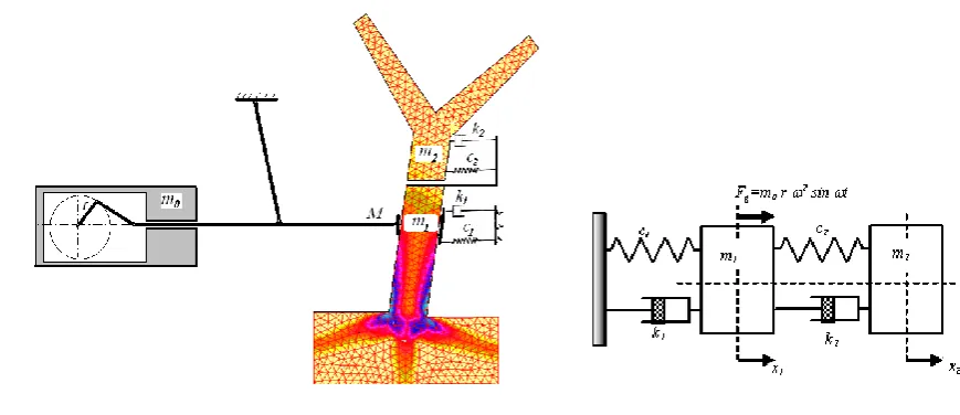
The two degree of freedom model of the fruit tree was
composed from one hand of the rooting system with a
certain amount of soil and of the trunk (index 1), from the
other hand of the main branches and limb moving
together when shaking the tree (index 2) , as is shown in
Figure 1.
Wherer
c1 is the spring constant of the trunk and routing system, m/N;
c2 is the spring constant of the main branches, m/N;
m1 is the reduced mass of the rooting system, soil around it and trunk, as well as the mass of shaker boom,
kg;
m2 is the reduced mass of the main branches and limb, kg;
k1 is the viscous damping coefficient of the trunk and routing system, Ns/m;
k2 is the viscous damping coefficient of the main branches, Ns/m;
m0 is the unbalanced mass of the inertia shaker, kg;
M is the mass of the shaker boom, kg;
R is the eccentricity of the unbalanced mass, m; is the angular velocity of the rotating unbalanced
mass, 1/s;
x1 and x2 are the displacements of the trunk and limb respectively, m;
Fg=m0r 2
sint is the periodical vibrating force, N. The kinetic system of equations for the model is as
follows:
t r m x c x k x c c x k k x
m ( ) (1 1) 1 2 0 2sin
2 2 2 1 2 1 1 2 1 1
1
(1) 0 1 1 1 2 1 2 2 2 2 2 2
2 x
c x k x c x k x
m
. (2)
Disregarding the description of the steps, after the
necessary transformations and substitutions, the
particular solution related to the mass m1 is:
) Ψ t ω sin( A x
x1= 1p = 1 + (3)
Where , 2 1 3 3 2 0 2 2 4 2 2 2 2 2 2 2 2 1 0 1 ) ω E ω E ( ) E ω E ω ( ) ω m k ( ) ω c m 1 ( ω r m m A -+ + -+ -= (4) a b arctg (5) 2 2 2 1 2 2 1 1 H H Z H Z H a , 2 2 2 1 2 1 1 2 H H Z H Z H b (6) ) ( 0 2 2 4
1 E E
H , ( 1 )
3 3
2 E E
H (7)
] 1 [ 2 2 2 2 1 0
1
c m r m m Z , 3 2 2 1 0 2 k r
m m m Z (8) 2 1 2 1 0 1 1 c c m m
E
, ] [ 1 2 1 1 2 2 1 1 c k c k m m
E
(9) ) ( 1 2 1 2 2 1 1 2 2 1
2 kk
c m m c m m m
E
(10) ] ) ( [ 1 2 2 1 1 2 2 1
3 m k m m k
m m
E
(11)
The kinetic equation for m2 can be written as
) 1 ( sin 1 1 1 1 1 1 2 0 2 2 x c x k x m t r m x
m
(12)
The particular solution for x2= x2p will result in:
) sin(
2
2A t
x (13)
Where, 2 2 2 B A , 2 2
2
J
K
B
(14) ] ) 1 ( [ 1 1 1 2 1 2 0 2
a kb
c m r m m
J
(15) ] ) 1 ( [ 1 1 2 1 1 2 b c m a k m
K
(16) J K arctg (17)
Finally for the accelerations applies:
) sin(
2
1 A t
a (18)
) sin(
2 2
2 A t
a (19)
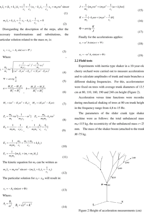
2.2 Field tests
Experiments with inertia type shaker in a 10-year-old
cherry orchard were carried out to measure accelerations
and to calculate amplitudes of trunk and main branches at
different shaking frequencies. For this, accelerometers
were fixed on trees with average trunk diameters of 13.5
cm at 80, 110, 160, 190 and 240 cm height (Figure 2).
Acceleration versus time functions were recorded
during mechanical shaking of trees at 80 cm trunk height
in the frequency range from 4,8 to 15 Hz.
The parameters of the slider crank type shaker
machine were as follows: the total unbalanced mass
m0=115 kg, the eccentricity of the unbalanced mass r=25 mm. The mass of the shaker boom (attached to the trunk)
M=75 kg.
The spring constants c1 of tested trunks were measured statically, applying different horizontal forces to them at
80 cm height. As the average value of three tests
resulted c1 =1.8 E-06 m/N as spring constant of the trunk. The three main branches (Figure 2) were regarded as
truncated cones contacted directly to the trunk by their
bottom end. The larger diameters were taken for 11 cm,
their smaller ones for 2.5 cm, their length 140 cm. The
center of gravity of a main brunch resulted for 38.5 cm
above their bottom end. The average spring constant c2 was measured by applying force to the branches at their
centre of gravity and recording their displacement. As a
result of tests the average spring constant of main
branches resulted in c2=7.0 E-06 m/N.
The reduced mass mr of the rooting system, soil around it and trunk was measured as follows: the limb of a
tree was removed at 80 cm height; the remaining trunk
was supplied with an accelerometer at its top. Then it
was displaced for about 25 mm horizontally and released.
Meanwhile acceleration versus time curve was recorded.
The action was repeated with an extra mass me, fixed to the top of the trunk. Acceleration versus time curve was
recorded in this arrangement as well. Using FTT the
natural frequencies f1 f2 of the two test arrangements was identified. Solving the Equation 20, called Rayligh’s
method, the mass mr could be calculated:
kg 385 1 f f
m m
2 2
2 1
e r
-= =
(20)
Where,
mr is the reduced mass of the rooting system, soil around it and trunk, kg;
f1and f2 are the natural frequency of the trunk without and with extra mass, Hz;
me = 13.5 kg, the extra mass.
With those data the trunk mass resulted in m1= mr +M=277+75=352 kg.
The reduced mass m2 of the main branches were calculated using the data achieved by determining the
centre of gravity of them. The total volume of the three
elements was 3,425 cm3, their total mass 28.5 kg.
The average dumping coefficient k1 was calculated off the running out acceleration versus time curves of the
shaken tree trunks, measured at 80 cm trunk height. The
equation applied (21):
(21)
Where,
m1 is the reduced mass of the rooting system, soil around it and trunk, as well as the mass of shaking rod,
kg;
Δ is the logarithmic decrement of the system,
measured on the diagrams;
tc is the cycle time of the vibration, s.
With the average logarithmic decrement of 1.26, cycle
time tc =0.08 s; the dumping coefficient k1 = 4012 Ns/m. The dumping coefficient of the main branches k2 was measured similarly to k1: the running out acceleration versus time curves of branches were evaluated.
Replacing Δ=0.82 into Equation (21), k2 = 705 Ns/m.
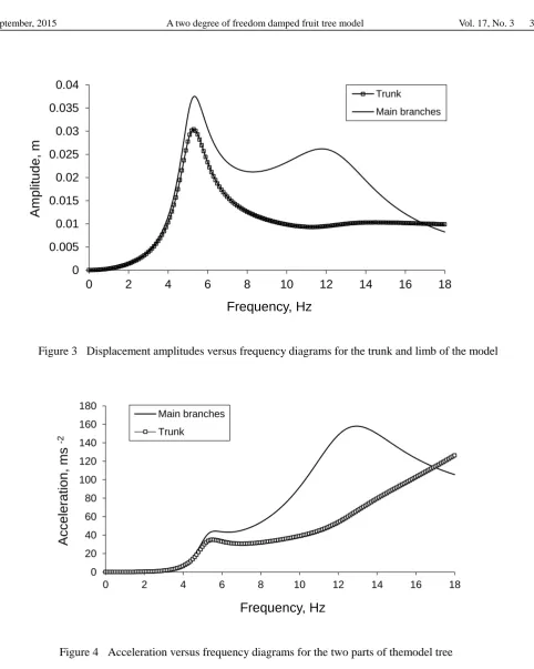
3 Results
By replacing shaker machine and fruit tree parameters
into Equations (1)-(19), displacement amplitude versus
frequency, as well as acceleration versus frequency
diagrams could be drawn for both trunk and main
branches of the model tree (Figures 3 and 4). As
expected, in both cases two natural frequencies are
recognizable, one at about 6 Hz, another at about 12 Hz.
Beyond the second natural frequency both the trunk and
limb displacement are decreasing. c
The theoretical average power demand of shaking the
model tree can be calculated, applying the Equation (22)
(Horváth and Sitkei, 2001):
3 2
2 , 1 2 , 1 av
,
s m A ω
2 1 P =
(22)
Where,
m1,2 are the reduced masses of trunk and main branches, respectively, kg;
A1,2 are the displacement amplitudes of trunk and main branches, respectively, m.
As the diagrams in Figure 5 indicate, the theoretical
average power demand of shaking for the trunk at the first
and second natural frequency is about the same. In case
of the limb, more power is used at 12 Hz than at 6 Hz. Figure 3 Displacement amplitudes versus frequency diagrams for the trunk and limb of the model
Figure 4 Acceleration versus frequency diagrams for the two parts of themodel tree
0 0.005 0.01 0.015 0.02 0.025 0.03 0.035 0.04
0 2 4 6 8 10 12 14 16 18
A
m
p
litu
d
e
,
m
Frequency, Hz
Trunk
Main branches
0 20 40 60 80 100 120 140 160 180
0 2 4 6 8 10 12 14 16 18
A
cce
lera
tio
n
,
m
s
-2
Frequency, Hz
Main branches
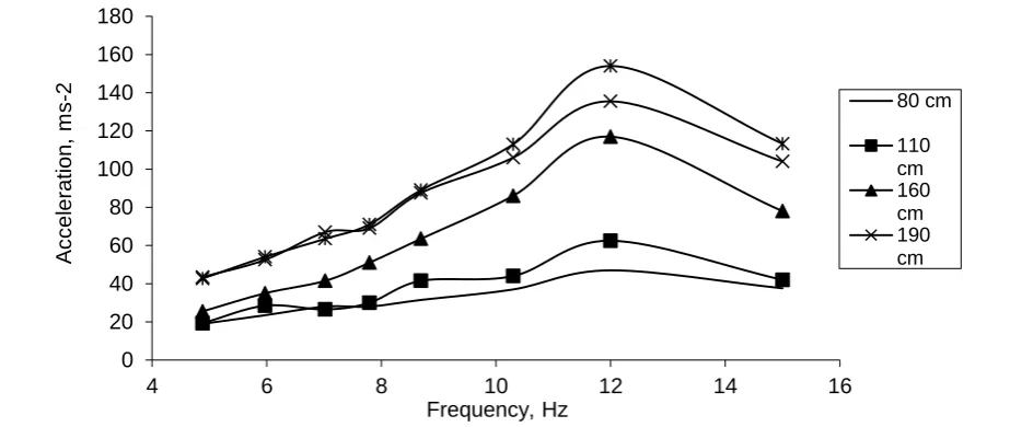
Figure 6 shows the acceleration values at different
heights of a real cherry tree between 4, 8 and 15 Hz
shaking frequencies. The first acceleration peak is
recognizable on three of five curves at 6 and 7 Hz
shaking frequencies, the second peak can be clearly
seen at 12 Hz at all curves.
Difference between measured and real acceleration
values can be recognised in the tendency of trunk
acceleration in the higher frequency range (Figures 4
and 6). The reason for this may be the dumping effect
of the foliage of the limb on real trees. Figure 5 Theoretical power demands for trunk and limb in function of shaking frequency
0 5 10 15 20 25 30
0 2 4 6 8 10 12 14 16 18
P
o
w
e
r d
e
m
a
n
d
,
kW
Frekvency, Hz
Main branches
Trunk
Figure 6 Acceleration versus frequency diagrams for the five different parts of a real cherry tree
0 20 40 60 80 100 120 140 160 180
4 6 8 10 12 14 16
A
c
c
el
erati
on
,
m
s
-2
Frequency, Hz
80 cm
The difference between measured and calculated first
and second resonance frequencies may be explained by
the asymmetry of the real tree structure and by the
inaccurate measuring methods of the parameters for trunk
and limb of the model tree.
4 Conclusions
The two degree of freedom model proved to be
applicable to describe a real fruit tree more accurate than
the model with one degree of freedom. It enables from
one hand to test the effect of shaker machine parameters,
such as unbalanced masses and the eccentricity of them as
well as the mass of shaker boom on limb amplitude and
acceleration.
From the other the natural frequencies of the
shaker-fruit tree system can be defined. For the practice
it means, that to achieve appropriate amplitude and
acceleration of the branches, the tree should be shaken at
its second natural frequency.
According to the diagram in Figure 3; shaking trees at
low frequencies large amplitudes can be achieved.
However, they don’t lead to high fruit detachment
because of the low acceleration at those frequencies.
The diagrams in Figure 5 indicate that the total power
use for shaking is much the same at about 6 and 12 Hz,
meanwhile the acceleration is much higher at 12 Hz
(Figures 4 and 6). This gives further argument to shake
the trees on their second natural frequency. Increasing
frequency further, more and more power would be used
for shaking the trunk, and less and less for the branches.
References
Bentaher, H., M. Haddar, T. Fakhfakh, and A. Mâalej. 2013. Finite elements modeling of olive tree mechanical harvesting using different shakers. Trees, (2013)27:1537-1545.
Castro-García, S., G. L. Blanco-Roldan, J. A. Gil-Ribes, J. Agüera-Vega. 2008. Dynamic analysis of olive trees in intensive orchards under forced vibration. Trees, (2008)22:795-802.
Fenyvesi, L., D. Fenyvesi. 2008. Optimization of a supporting device for mechanical harvesting. Acta Horticulturae, 768(55): 423-430.
Fridley, R. B., P. A. Adrian. 1966. Mechanical harvesting equipment for deciduous tree fruits. California Agricultural Experiment Station, Bulletin 825, 56. Galili, N., D. Rubinstein, and A. Shdema. 2001. Simulation
study and field test of adaptive trunk shaker for olives. Fruit, Nut, and Vegetable Production Engineering, 165-170, ISBN 3-00-008305-7 Institut für Agratechnik Bornim e. V.
Horváth, E., G. Sitkei. 2001. Energy consumption of selected tree shakers under different operational conditions. Journal of Agricultural Engineering Research, 80(2):191-199.