Classification and recognition scheme for vegetable pests based on the
BOF-SVM model
Deqin Xiao
1,2*,
Jianzhao Feng
1,
Tanyu Lin
1,
Chunhua Pang
1,
Yaowen Ye
1 (1. College of Mathematics and Informatics, South China Agricultural University, Guangzhou 510642, China; 2. Agricultural Aviation Research Institute of South China Agricultural University, Guangzhou 510642, China)Abstract: The current detection technology for vegetable pests mainly relies on artificial statistics, which exists many shortages
such as requiring a large amount of labor, low efficiency, feedback delay and artificial faults. By rapid detection and image processing technology targeting at vegetable pests, not only can reduce manpower and pesticide use, but also provide decision support for precise spraying and improve the quality of vegetables. Practical research achievements are still relatively lacking on the rapid identification technology based on image processing technology in vegetable pests. Given the above background, this paper presents a classification and recognition scheme based on the bag-of-words model and support vector machine (BOF-SVM) on four important southern vegetable pests including Whiteflies, Phyllotreta Striolata, Plutella Xylostella and Thrips. This paper consists of four sub-algorithms. The first sub-algorithm is to compute the character description of pest images based on scale-invariant feature transformation. The second sub-algorithm is to compute the visual vocabulary based on bag of features. The third sub-algorithm is to compute the classifier of pests based on support vector machines. The last one is to classify the pest images using the classifier. In this study, C++ and Python language were used as implementation technologies with OpenCV and LibSVM function library based on BOF-SVM classification algorithm. Experiments showed that the average recognition accuracy was 91.56% for a single image category judgment with 80 images from the real environment, and the average time was 0.39 seconds. This algorithm has achieved the ideal operating speed and precision. It can provide decision support for UAV precise spraying, and also has good application prospect in agriculture.
Keywords: agricultural image processing, vegetable pests, classification, recognition, bag of features, support vector machine
DOI: 10.25165/j.ijabe.20181103.3477
Citation: Xiao D Q, Feng J Z, Lin T Y, Pang C H, Ye Y W. Classification and recognition scheme for vegetable pests based
on the BOF-SVM model. Int J Agric & Biol Eng, 2018; 11(3): 190–196.
1 Introduction
The current detection technology for vegetable pests mainly relies on artificial statistics, which exists many shortages such as needing a large amount of labor, low efficiency, feedback delay, artificial faults and no decision support for pesticide spraying. By rapid detection and image processing technology targeting at vegetable pests, not only can it reduce manpower and pesticide use, but also provide decision support for precise spraying and improve the quality of vegetables. Recently, experts and scholars have conducted numerous studies on pests of rice, wheat, maize, canola and other major economic crops[1]. Nevertheless, practical
research achievements are still relatively lacking on the rapid identification technology of vegetable pests.
Image processing technology can improve the processing speed, and also increase the objectivity of the results and the reliability of the data. At the same time, it can save labor and reduce costs [2]. With the development of machine learning,
combining machine learning with image recognition has grown into
Received date: 2017-05-09 Accepted date: 2018-03-16
Biographies: Jianzhao Feng, PhD candidate, research interests: computer
engineering, Email: [email protected]; Tanyu Lin, MS, research interests: image processing, Email: [email protected]; Chunhua Pang,Lecturer, research interests: pest monitoring, Email: [email protected]; Yaowen Ye, MS, research interests: imaging processing, Email: [email protected].
*Corresponding author: Deqin Xiao, PhD, Professor, research interests:
computer vision, pest monitoring, internet of things. College of Mathematics and Informatics, South China Agricultural University, Guangzhou 510642, China. Tel: +86-20-85280320, Email: [email protected].
a hotspot for research and application in recent years. Watson et al.[3] used neural networks to automatically detect the field objects
of Lepidoptera. Vanhara[4] identified five Tachinidae by using
neural networks and morphological features. Cai Qing et al.[5]
used the BP neural network to identify seven morphological characters of vegetable pests. Lu et al.[1] used multi-template
matching and principal component analysis to identify the characteristics of rice pests, and the recognition rate has reached 83.1%. Wang[6] realized the recognition of wheat pests by
utilizing the LCV model combined with support vector machines, with a recognition rate of 81.25%. Wang[7] used feature
extraction to identify stored pests. Xu et al.[8] used the KL
transform combined with BP neural network to identify pests in fields. Xie et al.[9,10] proposed a method based on SVM for pest
pattern recognition.
Great research has been made on rice, wheat, maize, canola and other major economic pests in these years,, but results were still relatively lacking on vegetable pests, especially Whiteflies, Phyllotreta Striolata, Plutella Xylostella, Thrips and other southern pests. Considering the characteristics of insect pests, this paper proposes a scheme based on the bag-of-features model and support vector machines (BOF-SVM), in combination with the recognition of major pests in algorithms for classification of vegetables[11],
taking Whiteflies, Phyllotreta Striolata, Plutella Xylostella and Thrips as examples.
2 Materials and methods
2.1 Implementation environment and materials
2.49 and two libraries in LibSVM 3.20 under C ++ language environment, written by Professor Lin Zhiren at Taiwan University[12]. The images were derived from natural conditions,
as well as on-line materials, which contained different insect gestures, sizes, angles, and lighting. A total of 100 images were employed during the whole experiments. 20 training and test samples were used to generate the SVM classifier, and 80 were used to detect the target recognition effect of the generated classifier. From the 20 images, the feature parts of the target and background were extracted, and the pixels of the corresponding
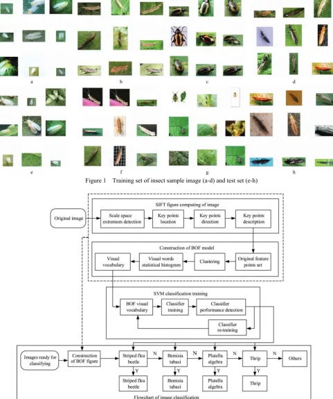
feature were extracted as the training samples of the classifier. The remaining pictures were extracted as the samples of the classifier. Parts of the materials were presented in Figure 1.
2.2 Pest recognition model
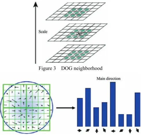
The algorithm was mainly described by the SIFT image descriptor combined with BOF-SVM. The algorithm was applied to identify and classify four vegetable pests in southern China, encompassing Whiteflies, Phyllotreta Striolata, Plutella Xylostella and Thrips. The overall structure of the algorithm model is presented in Figure 2.
a b c d
e f g h
Figure 1 Training set of insect sample image (a-d) and test set (e-h)
The entire process included two steps: the generation of the classifier and the recognition of vegetable pests. The classifier was composed of three steps: calculating the SIFT feature of the image, constructing the BOF model and SVM classifier and finally getting the corresponding pest category as output by following the above classifier image classification to identify and judge.
The rest of this paper will introduce how to implement four sub-algorithms: SIFT descriptor construction algorithms, the BOF visual vocabulary based on the SIFT algorithm, SVM-based classifier training algorithms and pest classification and recognition algorithms.
2.3 Image SIFT descriptor construction
Scale-invariant feature transform (SIFT) is an image feature descriptor algorithm published by Lowe in 1999[13] and optimized
in 2004[14]. It works by locating the farthest points in the spatial
scale and extracting their position, scale and rotation invariants. The key steps of the algorithm are as follows.
Step 1: Input ‘vegetable pest images’.
Step 2: SIFT feature points are calculated for each image, and feature point position information is obtained to form a candidate set of SIFT feature points. The detection of SIFT feature points is based on extreme points of scale space. For the detection point in DOG space, a total of 26 points are compared. These 26 points consist of 8 adjacent points and 18 points on the upper and lower adjacent scale. If the point has a value that is far outside of the norm, both in the DOG scale space and in the image’s two-dimensional space, it is considered as a characteristic point under the corresponding σ scale. This process is presented in Figure 3.
Step 3: Eliminate ‘noise’ as far as possible. Through methods such as interpolating neighboring data, discarding unclear points and eliminating edge response, select a subset of feature point candidate sets to obtain the SIFT feature points with more effective better anti-noise.
Step 4: Extract scale and direction information from the SIFT point set. At first, get the image L(x, y, σ) by Gaussian blurring processing; and then based on the dimension σ, gradient quantity
m(x, y), and direction θ(x, y), calculate the neighboring pixels using
2 2
( , ) ( ( 1, ) ( 1, )) ( ( , 1) ( , 1))
m x y = L x+ y −L x− y + L x y+ −L x y− and
( , ) arctan ( , 1) ( , 1), ( 1, ) ( 1, )
θ x y = L x y+ −L x y− L x+ y −L x− y . Step 5: Summarize all the gradients and directions within the neighbor pixels of each key point. Draw up a histogram to calculate the gradients and directions of the neighbor pixels of the key point. The histogram has been divided into 36 columns, each column representing a 10 degree span. The main direction of histogram is the same as the direction of its peak value, as showed in Figure 4.
Step 6: Based on these feature points, a SIFT image descriptor is generated to find the rest of the pest feature points. The first step is to determine the image region which is needed by descriptor calculating; then rotate coordinate axis to the key direction let descriptor with rotation invariance; meanwhile, assign the sample points to their corresponding sub-regions. The gradient in the sub-region is then projected on to the 4 × 4 window in 8 different directions. The weights of corresponding gradient were calculated, then using the difference method to obtain the gradient of each seed point in all 8 different directions. Finally, the feature description vector was sorted in accordance with the scale of feature points to acquire the finial SIFT descriptor. Figure 5 shows part of the SIFT descriptor generation process.
Figure 3 DOG neighborhood
Figure 4 Histogram of neighborhood direction of key points
Figure 5 SIFT descriptor generation process
2.4 Constructing BOF visual vocabulary
Currently, the ‘Bag of Features’ technique is commonly used for visual data classification of an image descriptor[15,16]; the word
collection methods commonly used are SIFT and SURF. In this paper, the SIFT method is utilized. The algorithm of constructing a SIFT-based bag of features is as follows.
Step 1: Detect SIFT feature points. The SIFT operator is to detect SIFT feature points from all images in the target sample set, and to determine information such as their positions, scales and direction gradients.
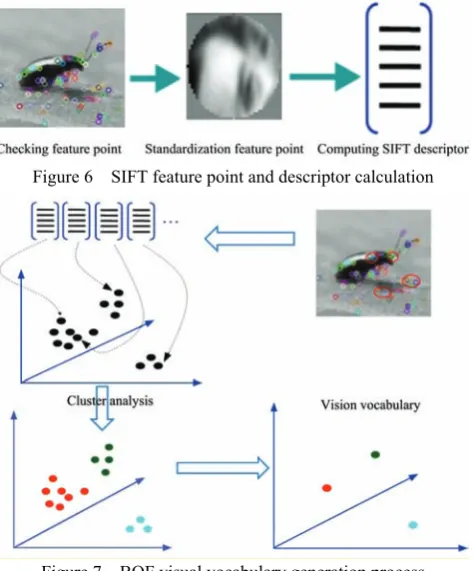
Step 2: Calculate the SIFT descriptor. Use the SIFT descriptor generation method to construct a 128-dimensional SIFT descriptor for every feature point from every image. The generation process for the descriptor is shown in Figure 6.
Step 3: Quantize the descriptor. Group all SIFT descriptors in the training sample set by using a k-means clustering algorithm. Descriptors in the same group shared some similarities, but those in different groups featured significant differences. The visual vocabulary of each image was its centre.
Step 4: Construct a visual vocabulary. Represent each element in the subset of the SIFT descriptor F = {F1, F2,…, Fm} by
a point using the nearest neighbor matching method, and the visual vocabulary is statistically represented by the nearest one. After the above processing, represent the image as I = {w1, w2, ……, wm}, in which wi represented the weight of the vocabulary set Fi of the image.
Step5: Generate BOF vocabularies for each image. Construct the BOF vocabularies by using the BOF model. The BOF vocabulary sets are generated in Figure 7.
with the BOF vocabularies in the image database, and calculate the angle between the two vocabularies. If it is less than a given threshold, the match is considered successful. The angle threshold can be chosen according to the experimental result.
Figure 6 SIFT feature point and descriptor calculation
Figure 7 BOF visual vocabulary generation process The advantages of using the BOF model to analyze the image are: 1) Through gathering statistical information, the total information contained in a given image can be reflected. This means that to a certain extent, the whole image can be described; 2) Through the general description of the image, it is possible to avoid storing a large number of local descriptors, thereby saving storage space. The disadvantages are: 1) The statistical information is general and the geometric information in between image regions are lost; 2) For each image, statistics and other operations need to be clustered together in order to calculate an increase in the final description of the image; 3) BOF model images must first be described as local features using the model to calibrate the system.
2.5 SVM classifier training based on the BOW
In this algorithm, because of the four insects involved, we needed to take one class of insects as the target, and the other three as the background, in order to train four classifiers[17]. In the later
stage of image classification, it can judge the BOF feature of the image by the four classifiers, and get the image classification result. The training algorithm of the SVM classifier based on BOF is shown below.
Step1: train the linear classifier. Use the non-negative Lagrangian coefficient αi to solve the constraint problem of
2 ,
1 arg min || ||
2
w b w in yi w x(( ⋅ i)− ≥b) 1 1≤ ≤i n , and find all
(( i ) 1 0
yi w x⋅ − − =b in
2
, 0 1
1
arg min max || || [ ( ) 1]
2
n
w b a≥ w i=a yi w xi i b
⎧ ⎫
− ⋅ − −
⎨ ⎬
⎩
∑
⎭.Step2: Solve the classifier function. For the equation
2
, 0 1
1
arg min max || || [ ( ) 1]
2
n
w b a≥ w i=a yi w xi i b
⎧ ⎫
− ⋅ − −
⎨ ⎬
⎩
∑
⎭ on thepartial derivatives of w and b respectively, make w=
∑
ni=1a y xi i iand
∑
nj=1a yj j=0 zero. Substitute the results into theequation 2
, 0 1
1
arg min max || || [ ( ) 1]
2
n
w b a≥ w i=a yi w xi i b
⎧ − ⋅ − − ⎫
⎨ ⎬
⎩
∑
⎭ ,and ( ) 1 1 ,
2
n T
i i j i j i j
i i j
L a% =
∑
=a −∑
a a y y x x will be obtained, where,
0 and 0
i i j i i
a ≥
∑
a y = . Solve the classifier function* 1
( ) sign{ n ( T ) }
i i i i
f x =
∑
=a y x x⋅ +b by using the equation* 1
( ) sign{ n ( T ) }
i i i i
f x =
∑
=a y x x⋅ +b .Step3: Carry out optimization training of a nonlinear classifier based on a kernel function. In order to obtain a higher dividing line, add a kernel function for a small number of linearly indivisible samples, and introduce the relaxation variable § to strike a balance between the training data and the unknown sample estimation by solving min || ||2
i i
w +C
∑
ξ in the case of y w xi( ⋅ − ≥ −i b) 1 ξi (1<i≤n), and obtaining the mapping kernel functionwhere is the sample space.
Step4: optimize parameters for SVM. Because the classifier function is not unique, the classifier has different generalization abilities due to different combinations of the penalty factor C and the kernel function parameter σ. C decides the generalization ability of the classifier and the sample fitting degree. The smaller the C value, the lower the classifier’s fitness to the training data, and the stronger the generalization ability. On the contrary, the lower the classifier's fitness to the sample, the worse the generalization ability. While the kernel function parameter σ
determines the number of support vectors, the smaller σ is, the more support vectors there will be; otherwise the greater σ is, the fewer support vectors there will be. Therefore, the choice of a useful pair of parameters can greatly improve the classification effect. This algorithm uses the grid method in SVM to find the parameter pair (C, σ) corresponding to the optimal generalization capability of the classifier. Then the unknown sample can be classified.
Step5: Classifier performance testing and re-training. Detect the classifier by using the predicted image samples. If the recognition rate is already high enough, utilize the current classifier for subsequent image processing. But if the performance is not good, we need to add the false image feature point set to the training set to re-train the classifier, so as to better the effect of subsequent image processing. The training method and generation process of SVM classifier based on BOF as shown in Figure 8.
Figure 8 SVM classifier generation process based on BOF
2.6 Classification and application of web pest image
Plutella Xylostella and Thrips, the classification and recognition algorithm can be constructed. Vegetable pest classification algorithm is shown below.
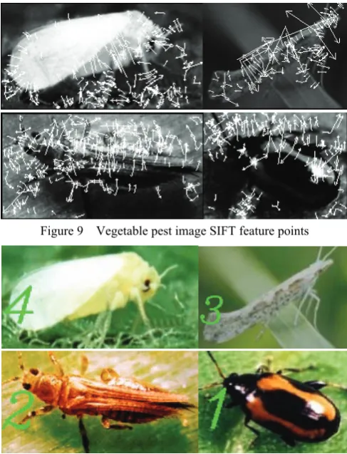
Step1: Compute the SIFT descriptor for the categorized image and obtain SIFT feature points and their corresponding descriptors by using the SIFT algorithm. The SIFT feature points are shown in Figure 9.
Step2: Solve Classified Images BOF Visual Vocabulary. Perform K-means clustering and statistical operations on the image SIFT descriptors to obtain the BOF visual vocabularies of the images to be classified.
Step3: Classifier generation and parameter optimization. Divide the training set into 5 parts, one of which are the training sets and the remaining four are the testing set. (C, σ) are optimized by the grid method, and the parameters optimized under the current training set are obtained. And four pests’ classifiers are obtained respectively, including Whiteflies, Phyllotreta Striolata, Plutella Xylostella and Thrips.
Step4: Classify pest images using the classifier. The resulting visual vocabulary of BOF is judged by the above four classifiers to obtain the final pest classification. The results of partial pest judgment are shown in Figure 10.
Figure 9 Vegetable pest image SIFT feature points
Note: 1. Phyllotreta Striolata; 2. Thrips; 3. Plutella Xylostella; 4. Whiteflies. Figure 10 Classifier final results
3 Experiment results
In the algorithm testing process, the images are collected from natural conditions of picturing and online material library. Materials of the insects contained various postures, sizes, lighting from different angles, etc. In order to verify this algorithm’s practicality and stability, a series of experiments are carried out, such as matching performance of SIFT feature points, analyzing classification training parameter examples, precision and operating speed of pest recognition, etc.
3.1 Matching performance of SIFT feature point
The experiment results showed that this algorithm can find out the SIFT feature points of four major pests well. The results of partial insect feature points search are shown in Figure 11. The starting point of the arrow in Figure 11 is the SIFT feature points. The arrow represents the direction as the length represents gradient.
Figure 11 SIFT feature points of some vegetable pests Finally, the SIFT image descriptor obtained from Plutella Xylostella images in the test sets. The experiment showed that the SIFT descriptor also had excellent stability and applicability. The experimental results are presented in Figure 12.
Figure 12 Effects of Target detection based on SIFT descriptor
3.2 Analysis of training result of classifier
After optimizing the parameters, the algorithm has gotten four classifier parameters (C, σ) corresponded by four types of insects including Whiteflies, Phyllotreta Striolata, Plutella Xylostella and Thrips. The classifier training procedures are shown in Figure 13.
Figure 13 Partial procedures and results of classifier training
3.3 Analyses the recognition accuracy of pests
The test set images were detected by the classifier, and parts of the results are shown in Figure 14.
From the classification results, even if the same pest whose size, angle, background, lighting and other factors in the environment are quite different, in most cases, the algorithm of the SVM classifiers trained by the BOF visual vocabulary could also recognize the target accurately.
morphological characteristics of two insects are similar. Some misjudgments are shown in Figure 15.
Note: 1. Phyllotreta Striolata; 2. Thrip; 3. Plutella Xylostella; 4. Whiteflies. Figure 14 Classification results of vegetable pests
Note: 2. Thrip; 3. Plutella Xylostella.
Figure 15 Error classification results of vegetable pest By classification testing, 80 images of 4 kinds of vegetable pests including the pests mentioned above have been identified, the exact quantity and its accuracy of the classification of test samples are shown in Table 1. According to the test samples, the average recognition accuracy of pests was 91.56%. To some extent, this experiment has confirmed the stability of SVM classifier based on SIFT descriptor. SVM classifier could ensure the accuracy of image recognition even under the influence of illumination or other noises.
Table 1 Accuracy rate of vegetable pests’ classification
Pests Numbers of samples
Accurate sample size
Recognition accuracy
Plutella Xylostella 80 74 92.50%
Thrips 80 72 90.00%
Phyllotreta Striolata 80 71 88.75%
Whiteflies 80 76 95.00%
Statistics 320 293 91.56%
3.4 Speed analysis of Algorithm
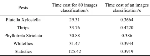
The time of classification is recorded during the experiment in classifying 80 images of 4 types of vegetable pests. The results are shown in Table 2. Table 3 shows that the average classification time for an image is about 0.4 seconds. If the density of the image data is not very large, the method could be workable.
Table 2 Time of vegetable pests’ classification
Pests Time cost for 80 images classification/s
Time cost of an images classification/s
Plutella Xylostella 29.31 0.3664
Thrips 33.76 0.4220 Phyllotreta Striolata 30.88 0.386
Whiteflies 31.47 0.3934 Statistics 125.42 0.3919
4 Conclusions
In this paper, the image description method based on SIFT image descriptor and BOF visual vocabulary is utilized to train the SVM, and the trained classifier is used to recognize and classify vegetable pests. The average accuracy rate of recognition classification is higher than 90% in many cases even if the test image contains a complex environmental background such as size, angle, etc. At the same time, the entire test set of 80 images can be classified in about 30 seconds, and each image takes 0.4 seconds on average. The experiments also show that misclassification only occurs in the case when the target feature is similar to the background features, or the shape is similar to other objects.
In conclusion, the algorithm which combines SVM with the image description method based on SIFT and BOF visual vocabulary can adapt to relatively complex environmental backgrounds and variable target shapes, and it has low noise sensitivity and certain stability. The algorithm is relatively efficient that can provide real-time decision support for precise spraying of cultivated UAV, and it also has a good application prospect in UAV fields. However, one disadvantage of SVM is that adding other pests does require modification of the model, and branches can be added continually to the classifier, as shown in Figure 2. So far, this program has just been implemented in the laboratory, but has not been applied to UAV in agricultural plant protection to provide accurate spraying services. In future studies, data generated by the classifier that identify the species and number of pests should be sent to a UAV spray controller through wireless transmission. Then it can provide data support for accurate spraying by that time.
Acknowledgments
This work was supported by the National Spark Program (2015GA780002) and Guangdong Province Science and Technology Program (2015A020224042). The authors would like to thank Liao Qin for her help with correcting grammatical errors.
[References]
[1] Lv J, Yao Q, Liu Q J, Xue J, Chen H M, Yang B J, et al. Identification of multi-objective rice light-trap pests based on template matching. China J Rice Sci, 2012; 26 (5): 619–623. (in Chinese)
[2] Lou D F, Zhang G M, Jiao Y, Liu X J, Chen Z L, Li Q F, et al. Research on insect image recognition with a common algorithm based on shape and texture. Plant Quarantine, 2012; 26 (4): 10–15. (in Chinese)
[3] Watson A T, O’Neill M A, Kitching I J. Automated identification of live moths (macrolepidoptera) using digital automated identification system (DAISY). Syst. Bio., 2004; 1(3): 287–300. (in Chinese)
[4] Vanhara J, Murarikova N, Malenovsky I, Havel J. Artificial neural networks for fly identification : A case study from the genera Tachina and Ectophasia (Diptera, Tachinidae). BIOLOGIA, 2007; 62(4): 462–469. [5] Cai Q. Research of vegetable leaf-eating pests based on image analysis.
MS dissertation, Yangling: Northwest A&F University, 2010; pp.13–34. (in Chinese)
[6] Wang L J. Research on the recognition method of wheat pest image based on LCV and SVM. Shanxi University of Science and Technology, 2013; pp.17–40. (in Chinese)
[7] Wang F. Study of feature extraction and recognition of stored product pests. MS dissertation. Qingdao: Qingdao University of Science & Technology, 2014; pp.11–37. (in Chinese)
[8] Xu X C, Zhao W P, Li C, Wang R P, Wang W. The farmland pests recognition algorithm based on KL transform and BP neural network. Shangxi Science and Technology, 2015; 30(2): 116–119, 132. (in Chinese) [9] Xie L B. Camellia pest image pattern classification method of the
University of Forestry & Technology, 2015; pp.14–39. (in Chinese) [10] Xie L B, Yu S J, Zhou G Y, Li H. Classification research of oil-tea pest
images based on BoW model. Journal of Central South University of Forestry & Technology, 2015; 35(5): 70–73. (in Chinese)
[11] Chang C, Lin C. LIBSVM: A library for support vector machines. ACM Transactions on Intelligent Systems and Technology (TIST), 2011; 2(3): 27.
[12] Lin Z R. LIBSVM: SVM classification toolkit. Taiwan University. Taiwan: 2015. http://download.csdn.net/detail/qq_27809141/8702367. Accessed on [2015-05-15].
[13] Lowe D. Object recognition from local scale invariant features. In: Seventh International Conference on Computer Vision (ICCV’99). IEEE Computer Society, 1999; 8(4): 1–8.
[14] Lowe D, Distinctive Image features from scale-invariant keypoints. International Journal of Computer Vision, 2004; 60(2): 91–110.
[15] Tan W X, Zhao C J, Wu H R. Intelligent alerting for fruit-melon lesion image based on momentum deep learning. Multimedia Tools and Applications, 2016; 75(24): 16741–16761.
[16] Deng X L, Lan Y B, Xing X Q, Mei H L, Liu J K, Hong T S. Detection of citrus Huanglongbing based on image feature extraction and two-stage BPNN modeling. Int J Agric & Biol Eng, 2016; 9(6): 20–26.