Comparative studies of methods of obtaining AGW’s propagation properties

Ann. Geophys., 30, 557–570, 2012 www.ann-geophys.net/30/557/2012/ doi:10.5194/angeo-30-557-2012

© Author(s) 2012. CC Attribution 3.0 License.

Annales

Geophysicae

Comparative studies of methods of obtaining

AGW’s propagation properties

H. Y. Lue1and F. S. Kuo2

1_{Department of Physics, Fu Jen University, Hsin Chuang, Taiwan}

2_{Department of Electro-Optical Engineering, Vanung University, Chung-Li, Taiwan} Correspondence to: F. S. Kuo ([email protected])

Received: 25 January 2011 – Revised: 5 January 2012 – Accepted: 10 February 2012 – Published: 19 March 2012

Abstract. Three among the existing methods of obtain-ing the properties (intrinsic period, wavelength, propaga-tion direcpropaga-tion) of atmospheric gravity waves (AGWs) were compared and studied by numerical method to simulate radar data. Three-dimensional fluctuation velocity satisfy-ing dispersion equation and polarization relation of atmo-spheric gravity wave were generated, then the numerical data were analysed by these methods to obtain the properties of waves. We found that, hodograph analysis was accurate for a monochromatic wave in obtaining its wave period and prop-agation direction, but the analysis became erratic for the case of multiple waves’ superposition. The error was especially large when data consisted of both upward propagating waves and downward propagating waves. The hodograph method became meaningful again if all the component waves propa-gated in the same direction and the resulting period was dom-inantly decided by the lowest frequency wave. Stokes pa-rameters method would obtain statistically meaningful val-ues of wave period and azimuth if the spreading of the az-imuths among the component waves did not exceed 90◦and the resulting period and azimuth were dominated by the low-est frequency wave component as well, irrespective of the vertical sense of propagation. Another method called phase and group velocity tracing technique was reconfirmed to be meaningful in measuring the characteristic wave period and vertical group and phase velocities of a wave packet: the characteristic wave period and vertical wavelength was dom-inated by the wave with the highest frequency among the component waves in the wave packet. Based on these nu-merical results, a composite procedure of data analysis for wave propagation was proposed and an example of real data analysis was presented.

Keywords. Meteorology and atmospheric dynamics

(Mid-dle atmosphere dynamics)

1 Introduction

There are many methods to obtain propagation properties of atmospheric gravity waves (AGWs), three of them hold our current interest: hodograph method, Stokes parameters method and the technique of phase and group velocity trac-ing. Hodograph analysis on a single monochromatic atmo-spheric gravity wave is accurate in obtaining its intrinsic frequency and propagation direction. According to polar-ization relation of gravity wave (in Northern Hemisphere), if the wave has a downward (upward) phase velocity, its hodograph-ellipse will have a clockwise (counter-clockwise) rotation, the ratio of the major to minor axis equals the fre-quency ratio ω

558 H. Y. Lue and F. S. Kuo: Comparative studies of methods of obtaining AGW’s propagation properties

well as the characteristic wave periods of wave packets can be obtained. Then the most probable characteristic intrinsic frequency, horizontal wavelength and azimuth of each wave packet can be found by fitting the dispersion equation and its related formula for vertical group velocity (Kuo et al., 2009). In this paper, we shall compare the merit and demerit of each method and try to find a composite procedure for obtaining the most probable propagation parameters of AGWs. One example of wave packet analysis of real radar data will be presented to demonstrate the procedure.

2 Formulation of gravity wainduced fluctuation ve-locities and Stokes parameters

The gravity wave induced 3-D fluctuation velocities must sat-isfy its Doppler relation (1a) and dispersion Eq. (1b) (Fritts and Alexander, 2003),

ω=σ−k·u0 , (1a)

m2= k

2_+`2

N2−ω2

ω2_−f2 −

1

4H2 , (1b)

and polarization relation (2a, 2b) (Gossard and Hooke, 1975; see also Kuo et al., 2009),

W = iω

N2_−ω2

ω2−f2 ωk+if·`

! ∂ ∂z+0

U

=ω ω

2_−f2

N2_−ω2 s

m2₊₀2 ω2_k2_+f2_`2×e

i(θ1+θ2)_×U

, (2a)

W = iω

N2_−ω2

ω2−f2 ω`−if·k

! ∂ ∂z+0

V

=ω ω

2_−f2

N2_−ω2 s

m2₊₀2 ω2_`2_+f2_k2×e

i(θ3+θ2)_{×V , (2b)}

or inversely,

U= N

2_−ω2

ω ω2_−f2 s

ω2_k2_+f2_`2 m2₊₀2 ×e

−i(θ1+θ2)_{×W, (3a)}

V= N

2_−ω2

ω ω2_−f2 s

ω2_`2_+f2_k2

m2₊₀2 ×e

−i(θ3+θ2)_{×W. (3b)}

Hereu0is the background wind velocity,kis the horizontal wave vector;U,VandWare the amplitudes of zonal, merid-ional and vertical velocities, respectively;σ,ω,k,`andm, respectively, are the observed frequency, intrinsic frequency, zonal-, meridional-, and vertical- wave number compo-nent. θ1=tan−1

ω·k f·`

,θ2=tan−1 m₀,θ3=tan−1

ω·`

−f·k

. 0∼=3.2×10−5radm (Eckart’s coefficient), N =2.09×

10−2rads (Brunt-Vaisala frequency, corresponding to 5 min

period), f ∼=8.31×10−5_rad

s (inertial frequency, corre-sponding to 21 h period, this value would exist for the latitude 30◦_{N) are assumed throughout this study. Then the vertical,}

zonal, and meridional components of fluctuation velocities w,uandv of a wave mode with intrinsic frequencyω, ob-served frequencyσ, wave numbersm,k and`were given by,

w=Wcos(kx+`y+mz−σ·t ), (4a)

u=Ucos(kx+`y+mz−σ·t )

= N

2_−ω2

ω ω2_−f2 s

ω2_k2_+f2_`2 m2₊₀2

·Wcos(kx+`y+mz−σ·t−θ1−θ2), (4b)

v=Vcos(kx+`y+mz−σ·t )

= N

2_−ω2

ω ω2_−f2 s

ω2_`2_+f2_k2 m2₊₀2

·Wcos(kx+`y+mz−σ·t−θ3−θ2) , (4c)

and,

˜

u=Ucos kx+`y+mz−σ·t−90◦

= N

2_−ω2

ω ω2_−f2 s

ω2_k2_+f2_`2 m2₊₀2

·Wsin(kx+`y+mz−σ·t−θ1−θ2), (4d)

whereu˜is a 90◦_{phase shift of zonal fluctuation velocity and}

was prepared for Stokes parameters analysis. The Stokes pa-rameters were given by,

I=Du2_+v2E _{, (5a)}

D=Du2_−v2E _{, (5b)}

P=2h_uvi _, (5c)

Q=2Duv˜ E, (5d)

where overbar denoted average over timetand angle bracket (<>)represented average over heightz. In optical terms,I is the throughout parameter,Dis the throughout anisotropic parameter,P is the linear polarization parameter andQis the circular polarization parameter.

3 Analysis of simulation data

Data generated from various models were analysed by the methods mentioned in Sect. 1. For simplicity of discussion, we would focus on the cases with negligible background wind in whichu0∼=0 andω∼=σ.

H. Y. Lue and F. S. Kuo: Comparative studies of methods of obtaining AGW’s propagation properties 559

3.1 Analysis of a single monochromatic wave

We generated vertical profiles of three wind components as well as the horizontal speed induced by a monochromatic wave (with downward phase velocity) characterised by τ=8h, λh=900 km, ϕaz= −45◦, λz= −8.70 km. (Parameters A)

Hereτ=2πωis the wave period,λhis the horizontal wave-length,φazis the azimuth of the wave vector, andλz is the vertical wavelength. A negative vertical wavelengthλz rep-resents a downward phase velocity (upward group velocity). Our analysis (not shown) confirmed that hodograph method was perfect for the case of a single monochromatic wave at each time step. This monochromatic wave data cannot be analysed by phase and group velocity tracing technique which is a method to analyse wave packet only.

In the following, we have a look at the results from the Stokes parameters method. The phase differenceδ(=θ3− θ1), major axis orientationφ (=90◦−φaz), the degree of po-larizationdand ellipse axis ratio AR were given by (Vincent and Fritts, 1987; Eckermann and Vincent, 1989),

δ=arctan QP, (6a)

2φ=arctan P D

, (6b)

d=D2+P2+Q21/2

I , (6c)

AR=cotξ where 2ξ=arcsin

Q d·I

. (6d)

The intrinsic wave period was found using τ= 2π

f·AR. (6e)

It is clear that Eq. (6b) cannot distinguish between the ma-jor axis orientation φ and φ±180◦, implying that Stokes parameters analysis cannot distinguish between eastward (northward) wave and westward (southward) wave. Also, Eqs. (6a)–(6e) cannot distinguish a phase-upward from a phase-downward propagating wave. The Stokes parameters analysis of oscillation data of the gravity wave characterised by Parameters A yielded thatτ=8 h,ϕaz= −45◦, andd=1, at each height. When the vertical sense of phase propagation of the wave in Parameters A was changed from downward to upward, or its azimuth was changed from−45◦_{to 135}◦_{, we}

obtained exactly same result (τ=8 h,ϕaz= −45◦andd=1, at each height) as expected. In general practice, the 180◦ -ambiguity in horizontal propagation direction can be solved by the correlation with simultaneous measurements of tem-perature oscillations (Kitamura and Hirota, 1989; Hamilton, 1991) due to the polarization between temperature, zonal and meridional wind (see e.g., Fritts and Alexander, 2003).

Table 1a. Properties of the AGWs to be superposed to generate

the perturbation velocities. Note: The negative sign ofλz means downward phase propagation.

j τ(h) λh(km) ϕaz ◦ λz(km) Aj

1 8 900 75 −8.701 0.1

2 8 900 75 +8.701 0.1α

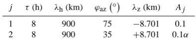
Table 1b. Same as Table 1a, but with different azimuth angles.

j τ(h) λh(km) ϕaz ◦ λz(km) Aj

1 8 900 75 −8.701 0.1

2 8 900 35 +8.701 0.1α

Table 1c. Same as Table 1b, but with identical vertical sense of

propagation.

j τ(h) λh(km) ϕaz ◦ λz(km) Aj

1 8 900 75 −8.701 0.1

2 8 900 35 −8.701 0.1α

3.2 Superposition of two waves with opposite vertical propagation

In the case of multiple waves’ superposition, the perturbation velocity is the vector sum of perturbation velocities of all the waves. So zonal, meridional, vertical perturbation velocities (u,v,w) and the 90◦phase shift of zonal fluctuation velocity

˜

uof the superposed waves were given by

u=X

j

Ajuj , (7a)

v=X

j

Ajvj , (7b)

w=X

j

Ajwj , (7c)

˜

u=X

j

Aju˜j , (7d)

withAj being the wave amplitudes. Now let us consider a special case of superposition of 2 AGWs whose properties were listed in Table 1a, and the perturbation velocities were given in Eq. (8a)–(8d),

u=0.1u1+0.1αu2 , (8a)

v=0.1v1+0.1αv2 , (8b)

560 H. Y. Lue and F. S. Kuo: Comparative studies of methods of obtaining AGW’s propagation properties

38   

Fig.1Height variations of perturbation velocities at successive times. Top panel: zonal velocity profile; Middle panel: meridional velocity profile; Bottom panel: vertical velocity profile. 5 

The data were obtained from the superposition of two monochromatic waves characterized in Table 1a with α =0.5 in equations (8a, 8b, 8c). The time step is 2.5 minutes and the height resolution is 150 meters. The vertical lines indicated 0 m/s for the first profile, and successive profiles are 50 minutes apart. The velocity scales are indicated below each panel.

10 

15 

0 100 200 300 400 500 600 700 800 900 1000 0

50 100 150 200

H

e

ig

h

t/

150

m

0 100 200 300 400 500 600 700 800 900 1000 0

50 100 150 200

He

ig

h

t/

1

5

0

m

0 100 200 300 400 500 600 700 800 900 1000 0

50 100 150 200

H

e

ig

h

t/

150

m

Time/2.5min 1 m/s

75 m/s 75 m/s

Fig. 1. Height variations of perturbation velocities at successive

times. Top panel: zonal velocity profile; middle panel: meridional velocity profile; bottom panel: vertical velocity profile. The data were obtained from the superposition of two monochromatic waves characterised in Table 1a withα=0.5 in Eqs. (8a), (8b), (8c). The time step is 2.5 min and the height resolution is 150 m. The verti-cal lines indicated 0 m s−1for the first profile and successive pro-files are 50 min apart. The velocity scales are indicated below each panel.

˜

u=0.1u˜1+0.1αu˜2 . (8d)

Notice that these 2 component waves in Table 1a had the same wave period, wavelength and azimuth angle, but had opposite vertical phase propagation. The major component wave (j=1)in Table 1a had downward phase velocity and the minor component wave (j =2)had upward phase ve-locity. The free parameterαis the amplitude ratio of minor to major component wave. We would present and compare three cases ofα=0.8,α=0.5 andα=0.25. Again, this ar-tificial data was not suitable for analysis by phase and group velocity tracing technique because there were too few waves to form credible wave packet.

3.2.1 Wave analysis by hodograph method

An example of the vertical profiles of zonal, meridional and vertical velocity obtained from Eqs. (8a), (8b), (8c) with am-plitude ratioα=0.5 shown on the top, middle and bottom panel, respectively, in Fig. 1, which clearly revealed down-ward phase propagation in all three panels. Their hodograph analyses were also made systematically at each time step. Almost all the hodographs could be perfectly fitted by el-lipses, among them, two examples of hodographs analysed at the 85th and 35th time step were presented in Fig. 2a and b, respectively, both hodographs had clockwise

rota-39   

Fig.2a Hodograph analysis of vertical profiles of three wind components and the horizontal velocity

5 

amplitude induced by the superposition of two waves characterized by Table 1a with α=0.5 in equations (8a, 8b, 8c) at the 85th time step. The rotation sense of this hodograph is clockwise (from green circle to red square to blue cross). τ=8.25hr and 106.6φ =az ° were obtained by this analysis.

10 

15 

-20 -15 -10 -5 0 5 10 15 20

-20 -15 -10 -5 0 5 10 15 20

u(m/s)

v(

m

/s

)

Fig. 2a. Hodograph analysis of vertical profiles of three wind

com-ponents and the horizontal velocity amplitude induced by the su-perposition of two waves characterised by Table 1a withα=0.5 in Eqs. (8a), (8b), (8c) at the 85th time step. The rotation sense of this hodograph is clockwise (from a green circle to a red square to a blue cross).τ=8.25 h andφaz=106.6◦were obtained by this analysis.

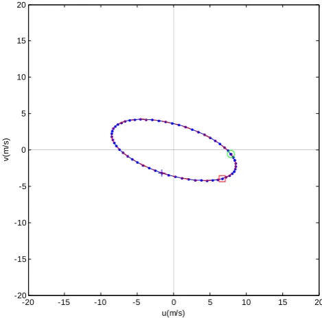
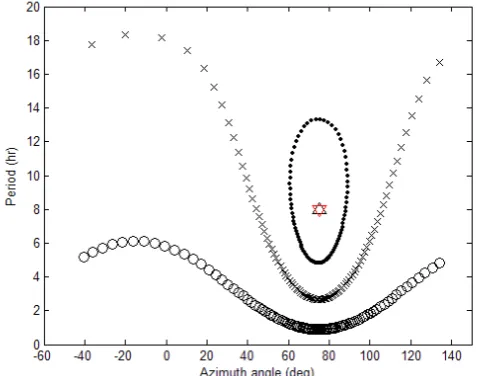
tion. Hodograph analysis in Fig. 2a resulted in τ=8.25 h andφaz=106.6◦, and the corresponding analysis of Fig. 2b resulted inτ=3.17 h andφaz=65.4◦. These two examples revealed that either the wave period (3.17 h in Fig. 2b) or the azimuth (106.6◦ in Fig. 2a) obtained by hodograph analy-sis was far too different from the true values (i.e.,τ=8 h, φaz=75◦). A detailed hodograph analysis at each time step of Fig. 1 was summarized in Fig. 3, which showed the pe-riod vs. azimuth plots of all the results of hodograph analysis (by cross) along with the corresponding results of two other cases withα=0.8 (represented by open circle) andα=0.25 (represented by dot) and the original component waves (by upward triangle and downward triangle). To distinguish the direction of vertical propagation, the event with downward phase velocity was represented by a black symbol, while the event with upward phase velocity was represented by a red symbol. Figure 3 clearly demonstrated that the vertical prop-agation of all the resulting waves under study were the same as their major component wave (in terms of amplitude), i.e., downward phase propagation. Even if the amplitude ratioα was as large as 0.8, the vertical sense of propagation of the resulting wave was still completely dominated by the major wave. Also, the error in the azimuth and wave period resulted from hodograph analysis decreased with decreasingα, and the error was so large that even if this amplitude ratio was as small as 0.25, the error was still too large to be acceptable.

H. Y. Lue and F. S. Kuo: Comparative studies of methods of obtaining AGW’s propagation properties Fig. 2b 561

-20 -10 0 10 20

-20 -15 -10 -5 0 5 10 15 20

u(m/s)

v(

m

/s)

Table 5

ID Major axis

a (m/s)

Minor axis

b (m/s) τ

( )

( )

1 22.039 9.006 8.581 −84.3

2 18.849 7.962 8.871 −76.3

3 26.304 22.786 18.191 −43.9

4 30.445 24.622 16.984 58.1

5 26.630 12.006 9.467 89.5

6 23.392 9.174 8.236 −89.8

7 19.066 8.020 8.834 −75.4

8 27.328 23.072 17.73 −53.4

9 30.699 25.395 17.372 60.7

10 23.990 12.335 10.797 82.3

11 21.514 12.989 12.679 −53.5

12 24.085 21.100 18.398 −65.0

13 28.066 20.673 15.451 63.3

Fig. 2b. Same as Fig. 2a except at the 35th time step. The rotation

sense of this hodograph is clockwise (from a green circle to a red square to a blue cross). τ=3.17 h andφaz=65.4◦were obtained by this analysis.

From the examples above, we concluded that superposi-tion of two waves with the same period and wavelengths, but opposite vertical propagation would misleadingly yield hodographs perfectly fitted by ellipses with erroneous wave period and azimuth even though they propagated in same horizontal direction. Further studies showed that, additional error would result if the azimuths of these two component waves also differed. For example, a difference of 40 degrees in azimuths between the two waves as defined in Table 1b would contribute an additional 1 h of error in wave period and 10 degrees of error in azimuth.

3.2.2 Wave analysis by Stokes parameters method

The results of Stokes parameters analyses of three cases of zonal and meridional velocities, which were defined by Eqs. (8a), (8b), (8d) and Table 1a with amplitude ratioα=

0.8, 0.5, and 0.25, were all the same at each height (without doing height averages in Eqs. 5a, 5b, 5c, 5d):τ=8 h,ϕaz= 75◦_{andd=1, which was exactly the same as a}

monochro-matic wave in Table 1a irrespective of its vertical sense of propagation. This result was a natural consequence of Stokes parameters analysis because it could not identify the vertical sense of gravity wave propagation. When the azimuths of the two waves were separated by 40◦as shown in Table 1b, the results of Stokes parameters analyses were as follows: for the case ofα=0.8, we obtainedτ=9.46 h,ϕaz=60.1◦and d=0.88; for the case ofα=0.5, we obtainedτ=8.86 h, ϕaz=68.2◦andd=0.92; for the case ofα=0.25, we

ob-41   

5 

Fig.3 Plot of period vs. azimuth angle resulted from hodograph analysis of equations (8a,8b, 8c); at each time step of three cases and the original waves. Open circle represents the results from the 10 

case with α =0.8 in equations (8a,8b, 8c); Cross represents the results from the case with 0.5

α = ; and dot represents the results from the case with α =0.25. Black upward pointing triangle represents original wave with downward phase velocity (first wave in Table 1a) and red downward pointing triangle represents the original wave with upward phase velocity (second wave in Table 1a).

15 

20 

Fig. 3. Plot of period vs. azimuth angle resulted from hodograph

analysis of Eqs. (8a), (8b), (8c) at each time step of three cases and the original waves. An open circle represents the results from the case withα=0.8 in Eqs. (8a), (8b), (8c); a cross represents the re-sults from the case withα=0.5; and a dot represents the results from the case withα=0.25. A black upward pointing triangle rep-resents original wave with downward phase velocity (first wave in Table 1a) and a red downward pointing triangle represents the orig-inal wave with upward phase velocity (second wave in Table 1a).

tainedτ=8.27 h,ϕaz=73.2◦andd=0.97. The results re-vealed that the superposition of two waves of the same period and wavelengths with opposite vertical sense of propagation and different azimuth tended to increase the characteristic wave period and decrease the degree of polarization. And the resulting azimuth was close (but not equal) to the weight-ing average of their azimuth angles. Here we must emphasize that when height averages on the Stokes parametersI,D,P, Qin Eqs. (5a)–(5d) were not taken, the results of intrinsic period, azimuth angle and the degree of polarization at each height were varying in height with large fluctuations.

562 H. Y. Lue and F. S. Kuo: Comparative studies of methods of obtaining AGW’s propagation properties

42   

5 

Fig.4 Period vs. vertical wavelength plot of the component waves in Table 2a (by upward triangle) and the investigations of wave packets such as that in Fig.7 by phase and group velocity tracing 10 

technique (by cross). When all the component waves in Table 2a propagate in same direction with azimuth of 20 degrees (Table 2c), the velocity tracing investigations of the corresponding wave packets were presented by ‘dot’.

15 

20 

Fig. 4. Period vs. vertical wavelength plot of the component waves

in Table 2a (by upward triangle) and the investigations of wave packets such as that in Fig. 7 by phase and group velocity tracing technique (by a cross). When all the component waves in Table 2a propagate in same direction with azimuth of 20 degrees (Table 2c), the velocity tracing investigations of the corresponding wave pack-ets were presented by a “dot”.

43   

5 

Fig.5 Period vs. azimuth plot of the component waves in Table 2a (by black upward triangle) and

10 

the results of hodograph analysis (by blackcross) around each wave packets as listed in Table 3. When all the component waves in Table 2a propagate in same direction with azimuth of 20 degrees (see Table 2c) as shown by green upward triangle, the corresponding hodograph analyses were presented by ‘green dot’.

15 

20 

Fig. 5. Period vs. azimuth plot of the component waves in Table 2a

(by a black upward triangle) and the results of hodograph analysis (by a black cross) around each wave packets as listed in Table 3. When all the component waves in Table 2a propagate in same di-rection with azimuth of 20 degrees (see Table 2c) as shown by a green upward triangle, the corresponding hodograph analyses were presented by a “green dot”.

(i.e.,φ=(φ1+αφ2)(1+α)). Almost the same results of wave period and azimuth were also obtained by hodograph analysis. So, it would be better if upward- and downward-propagating waves were separately treated by Stokes

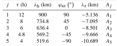
param-Table 2a. Properties of five upward propagating AGWs with 180◦

azimuth spreading to be superposed.

j τ(h) λh(km) ϕaz ◦ λz(km) Aj

1 12 900 90 −5.136 A1

2 8 734.8 45 −7.095 A2

3 6 636.4 0 −8.501 A3

4 4.8 569.2 −45 −9.666 A4 5 4 519.6 −90 -10.689 A5

Table 2b. Same as Table 2a, but for 90◦azimuth spreading only.

j τ(h) λh(km) ϕaz ◦ λz(km) Aj

1 12 900 90 −5.136 A1

2 8 734.8 67.5 −7.095 A2

3 6 636.4 45 −8.501 A3

4 4.8 569.2 22.5 −9.666 A4

5 4 519.6 0 −10.689 A5

Table 2c. Same as Table 2a, but for identical azimuth angles.

j τ(h) λh(km) ϕaz ◦ λz(km) Aj

1 12 900 20 −5.136 A1

2 8 734.8 20 −7.095 A2

3 6 636.4 20 −8.501 A3

4 4.8 569.2 20 −9.666 A₄

5 4 519.6 20 −10.689 A5

eters analysis, but it is necessary that upward and downward waves must be separately treated by hodograph analysis.

3.3 Superposition of five upward propagating waves

Now let’s consider the case of superposition of 5 downward phase velocity AGWs whose properties were listed in Ta-ble 2a, and indicated by black upward triangle in the period vs. vertical wavelength plot of Fig. 4 and in the period vs. azimuth plot of Fig. 5. Notice that each wave in Table 2a had different azimuth, period and wavelength, and its am-plitudeAj would be defined case by case. The perturbation velocity profiles obtained by Eqs. (7a), (7b), (7c), (7d) with A1=A2=A3=A4=A5=0.1 (to be referred as Case M1 hereafter) were presented in Fig. 6a and b. The former one (Fig. 6a) presenting the time variations of perturbation ve-locities at successive heights, was prepared for phase and group velocity tracing analysis and Stokes parameters analy-sis; while the later (Fig. 6b) presenting the height variations of perturbation velocities at successive times, was prepared for hodograph analysis.

H. Y. Lue and F. S. Kuo: Comparative studies of methods of obtaining AGW’s propagation properties 563

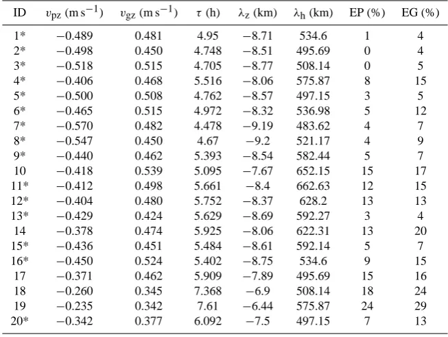
Table 3. Results of wave packet analysis. Vertical wavelengthλzwith negative sign indicates downward phase propagation. The star (*) sign indicates the event satisfies dispersion equation under following condition:v_gz− ˜v_gz

vgz

<0.15 and

v_pz− ˜v_pz

vpz

<0.15. EG and EP are, respectively, the percentage error of vertical group and phase velocities:

EG=vgz− ˜vgzvgz×100 % EP=

vpz− ˜vpzvpz×100 %

ID vpz(m s−1) vgz(m s−1) τ(h) λz(km) λh(km) EP (%) EG (%)

1* −0.489 0.481 4.95 −8.71 534.6 1 4

2* −0.498 0.450 4.748 −8.51 495.69 0 4

3* −0.518 0.515 4.705 −8.77 508.14 0 5

4* −0.406 0.468 5.516 −8.06 575.87 8 15

5* −0.500 0.508 4.762 −8.57 497.15 3 5

6* −0.465 0.515 4.972 −8.32 536.98 5 12

7* −0.570 0.482 4.478 −9.19 483.62 4 7

8* −0.547 0.450 4.67 −9.2 521.17 4 9

9* −0.440 0.462 5.393 −8.54 582.44 5 7

10 −0.418 0.539 5.095 −7.67 652.15 15 17

11* −0.412 0.498 5.661 −8.4 662.63 12 15

12* −0.404 0.480 5.752 −8.37 628.2 13 13

13* −0.429 0.424 5.629 −8.69 592.27 3 4

14 −0.378 0.474 5.925 −8.06 622.31 13 20

15* −0.436 0.451 5.484 −8.61 592.14 5 7

16* −0.450 0.524 5.402 −8.75 534.6 9 15

17 −0.371 0.462 5.909 −7.89 495.69 15 16

18 −0.260 0.345 7.368 −6.9 508.14 18 24

19 −0.235 0.342 7.61 −6.44 575.87 24 29

20* −0.342 0.377 6.092 −7.5 497.15 7 13

3.3.1 Phase and group velocity tracing analysis

The vertical group velocityvgz, vertical phase velocityvpz, and the characteristic wave periodτ of a wave packet were determined directly by the technique of phase and group ve-locity tracing (see Sect. III of Kuo et al., 2003) and the ob-served wave frequencyσ and vertical wave numbermwere obtained readily byσ=1τ andm=σvpz, respectively.

A partial range-time plot of(δV )2 derived from the left panel of Fig. 6a was shown in Fig. 7, where 10 wave packets were identified and determined by phase and group velocity tracing technique. A total number of 20 wave packets (10 fromu-profile and 10 fromv-profile) were investigated and the results of investigations were listed in Table 3 and pre-sented by cross in Fig. 4. Among these 20 events, 15 of them (denoted by a star in Table 3) satisfied the dispersion equa-tion under following condiequa-tion:

vgz− ˜vgz

vgz

<0.15 and

vpz− ˜vpz

vpz

<0.15. (9)

(Herev˜gz andv˜pzwere theoretical values of vertical group and phase velocity best fitted by dispersion equation). Their mean values of the characteristic wave periods, vertical wavelengths and horizontal wavelengths were obtained to be 5.21 h, −8.55 km and 549.5 km with small standard devia-tions of 0.49 h, 0.42 km and 53.6 km, respectively. These mean values were closely associated withj=3 and j=4

wave (representing higher frequency part among the compo-nent waves) in Table 2a. One should not expect these wave packet analyses to be perfect, because the wave packets in this study were formed from five discrete waves with differ-ent horizontal wavelengths. However, the theoretical vertical group velocity was defined by partial derivative of frequency with respect to vertical wave number at constant horizontal wave vector as follows,

vgz= ∂σ

∂m=

∂ω

∂m=

−m ω2−f2

ω

k2+`2+m2+ 1

4H2

. (10)

564 H. Y. Lue and F. S. Kuo: Comparative studies of methods of obtaining AGW’s propagation properties

44   

5 

Fig.6a Time variations of perturbation velocities at successive heights. Left panel: zonal velocity profile; Middle panel: meridional velocity profile; Right panel: vertical velocity profile. The data were obtained from equations (7a,b,c) and Table 2a with

1 2 3 4 5

(A A A A A, , , , )=(0.1, 0.1, 0.1, 0.1, 0.1).The time step is 2.5 minutes and the height

resolution is 150 meters. The horizontal lines indicate 0 m/s for the first profile, and

10 

successive profiles are 0.75 km apart. The velocity scales of zonal and meridional velocities are indicated at the lower left corner of this figure, and the velocity scale of the vertical velocity is indicated at the lower right corner of this figure. These velocity profiles were prepared for wave packet analysis (phase and group velocity tracing technique) and Stokes parameters analysis.

15 

0 500 1000 0 20 40 60 80 100 120 140 160 180 200 H e ight /150 m time/2.5min

0 500 1000 0 20 40 60 80 100 120 140 160 180 200 Time/2.5min

0 500 1000 0 20 40 60 80 100 120 140 160 180 200 Time/2.5min 2 m/s 100 m/s

Fig. 6a. Time variations of perturbation velocities at successive

heights. Left panel: zonal velocity profile; middle panel: merid-ional velocity profile; right panel: vertical velocity profile. The data were obtained from Eqs. (7a), (7b), (7c) and Table 2a with

(A1,A2,A3,A4,A5)=(0.1,0.1,0.1,0.1,0.1). The time step is 2.5 min and the height resolution is 150 m. The horizontal lines indicate 0 m s−1 for the first profile, and successive profiles are 0.75 km apart. The velocity scale of zonal and meridional velocities are indicated at the lower left corner of this figure, and the velocity scale of the vertical velocity is indicated at the lower right corner of this figure. These velocity profiles were prepared for wave packet analysis (phase and group velocity tracing technique) and Stokes parameters analysis.

A3=0.06,A4=0.08,A5=0.1. In each case, 20 wave pack-ets were investigated, andn(case by case) out of the 20 wave packets satisfied condition (9). The results of cases M1– M6 were summarized in Table 4, which revealed that the characteristic parameters of the wave packets were all dom-inated by the higher frequency wave components. It should be emphasized here that in windless situation, the azimuth of wave propagation cannot be determined from the disper-sion Eq. (1b). If non-negligible background wind veloc-ity is known, two azimuths symmetric with respect to the background wind velocity direction can be obtained from Eqs. (1a), (1b) and (10). And the true azimuth can be de-termined from these two symmetric azimuths with the help of momentum flux measurement (Kuo et al., 2009).

3.3.2 Hodograph analysis

To make comparison with the results from the phase and group velocity tracing technique, we made hodograph anal-ysis around each wave packet (in terms of time and height range) in Table 3. The senses of rotations of all the hodographs were found to be clockwise, meaning down-ward phase velocity as expected. One example of hodograph (ID = 13 in Table 3) was shown in Fig. 8, whose major to

45   

5 

Fig.6b Height variations of perturbation velocities at successive times. Top panel: zonal velocity profile; Middle panel: meridional velocity profile; Bottom panel: vertical velocity profile. The time step is 2.5 minutes and the height resolution is 150 meters. The data were obtained from equations (7a,b,c) and Table 2a with

1 2 3 4 5

(A A A A A, , , , )=(0.1, 0.1, 0.1, 0.1, 0.1). The vertical lines indicated 0 m/s for the first

10 

profile, and successive profiles are 50 minutes apart. The velocity scales are indicated at the bottom of each panel. These velocity profiles were prepared for hodograph analysis.

15 

0 100 200 300 400 500 600 700 800 900 1000 0 50 100 150 200 H e ig h t/ 150 m

0 100 200 300 400 500 600 700 800 900 1000 0 50 100 150 200 He ig h t/ 1 5 0 m

0 100 200 300 400 500 600 700 800 900 1000 0 50 100 150 200 H e ig h t/ 150 m Time/2.5min 220 m/s

220 m/s

2.2 m/s

Fig. 6b. Height variations of perturbation velocities at successive

times. Top panel: zonal velocity profile; middle panel: merid-ional velocity profile; bottom panel: vertical velocity profile. The time step is 2.5 min and the height resolution is 150 m. The data were obtained from Eqs. (7a), (7b), (7c) and Table 2a with

(A1,A2,A3,A4,A5)=(0.1,0.1,0.1,0.1,0.1). The vertical lines in-dicated 0 m s−1 for the first profile, and successive profiles are 50 min apart. The velocity scales are indicated at the bottom of each panel.. These velocity profiles were prepared for hodograph analysis.

46   

5 

Fig.7 A partial range-time plot of ( )δV 2of zonal velocity converted from left panel of Fig.6a.

Determinations of vertical phase and group velocities of wave packets were indicated by the phase lines (along the patch) and energy lines (across the patch).

10 

15 

20 

Fig. 7. A partial range-time plot of(δV )2of zonal velocity con-verted from left panel of Fig. 6a. Determinations of vertical phase and group velocities of wave packets were indicated by the phase lines (along the patch) and energy lines (across the patch).

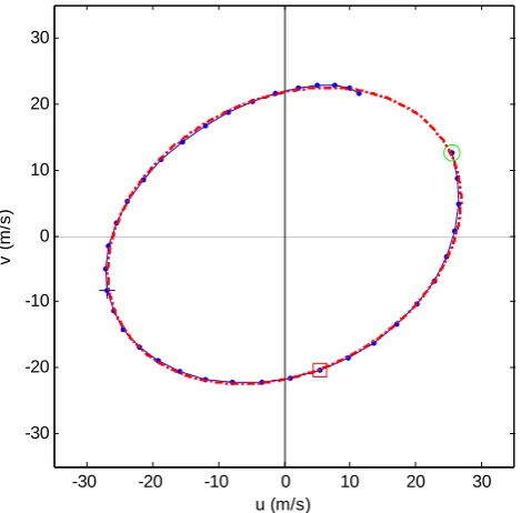
minor axis ratio yields an intrinsic period of 15.45 h, and its major axis lay along the direction with ϕaz=63.3◦. This intrinsic period is larger than each of the original wave in

H. Y. Lue and F. S. Kuo: Comparative studies of methods of obtaining AGW’s propagation properties 565

47   

5 

10 

Fig.8 Hodograph at t=250Δt and height range 105Δ −z 141Δz _{of Fig.6b. Least square fitting}

by an ellipse yields τ =15.45hr and ϕ_az=63.3°. The rotation sense of this hodograph is

clockwise.

15 

20 

-30 -20 -10 0 10 20 30

-30 -20 -10 0 10 20 30

u (m/s)

v (

m

/s)

Fig. 8. Hodograph att=2501tand height range 1051z−1411z of Fig. 6b. Least square fitting by an ellipse yieldsτ=15.45 h and

ϕaz=63.3◦. The rotation sense of this hodograph is clockwise.

Table 4. Results of phase and group velocity analysis: the number of wave packets n satisfying condition (9), and their mean±standard deviation of their intrinsic periodτ (h), vertical wavelengthλz(km), and horizontal wave lengthλh(km).

n τ λz λh

Case M1 15 5.21±0.49 −8.55±0.42 549.5±53.6 Case M2 15a 6.18±0.49 −8.61±0.38 665.8±53.6 Case M3 14 4.91±0.52 −9.16±0.30 553.7±64.3 Case M4 12 5.19±0.57 −8.90±0.53 567.2±47.8 Case M5 10 5.18±0.28 −8.61±0.28 550.4±45.8 Case M6 17 4.89±0.66 −9.22±0.44 552.7±73.6 a _{Actually, there were only 6 wave packets satisfying Eq. (9) in} Case M2, so we relaxed the condition from 0.15 to 0.20 in Eq. (9) to increase the number of wave packets.

Table 2a. The results of hodograph analysis for all the wave packets were listed in Table 5 and presented by a “cross” in the period vs. azimuth plot in Fig. 5, which revealed that half of the hodographs yielded wave periods well beyond the spectrum of the input waves in Table 2a. We also noticed that the hodograph in Fig. 8 was not complete, because those data points that deviated away from the ellipse were removed from the dataset and the remaining data were refitted again by an ellipse. Such fitting process was repeated until best fit-ting was reached. Actually, none of the hodographs in this case was complete. So we did not proceed to make hodo-graph analysis for Cases M2–M6.

Table 5. Results of hodograph analysis corresponding to each wave

packet in Table 3.

ID Major axis Minor axis τ(h) ϕaz ◦ a (m s−1) b (m s−1)

1 22.039 9.006 8.581 −84.3 2 18.849 7.962 8.871 −76.3 3 26.304 22.786 18.191 −43.9 4 30.445 24.622 16.984 58.1 5 26.630 12.006 9.467 89.5 6 23.392 9.174 8.236 −89.8 7 19.066 8.020 8.834 −75.4 8 27.328 23.072 17.73 −53.4 9 30.699 25.395 17.372 60.7 10 23.990 12.335 10.797 82.3 11 21.514 12.989 12.679 −53.5 12 24.085 21.100 18.398 −65.0 13 28.066 20.673 15.451 63.3 14 30.092 17.056 11.903 66.7 15 22.906 16.856 15.453 −57.3 16 25.669 22.061 18.048 66.9 17 29.422 18.878 13.474 66.0 18 23.314 12.022 10.829 78.6 19 24.896 13.481 11.371 78.4 20 16.775 9.665 12.099 83.0

Table 6. Results of Stokes parameters analysis: intrinsic period,τ

(h),ϕaz(◦), and degree of polarizationd.

τ ϕaz d

Case M1 14.48 80.9 0.80 Case M2 13.29 82.6 0.89 Case M3 14.89 88.7 0.69 Case M4 12.50 74.0 0.85 Case M5 12.02 82.3 0.94 Case M6 13.29 51.3 0.72

3.3.3 Stokes parameters analysis

The result of Stokes parameters analyses of Cases M1–M6 were all height independent and the results of intrinsic pe-riodτ (h), azimuth angleϕaz(◦)and degree of polarization d at each height were summarized in Table 6. The results of Case M2 and Case M3 were contradictory: The azimuth of the largest amplitude wave in Case M3 was−90◦_{, while}

566 H. Y. Lue and F. S. Kuo: Comparative studies of methods of obtaining AGW’s propagation properties

(Cases M4–M6), the results were reasonable and we could conclude that both the resulting period and azimuth were dominated by the largest period wave. The fact that the re-sulting intrinsic periods were all larger than the longest pe-riod (12 h) among the component waves was believed to be resulted from the azimuth spreading among the component waves.

3.4 Superposition of five waves propagating in same direction vertically and horizontally

A special case related to the previous cases was the superpo-sition of five waves with same amplitude (A1=A2=A3= A4=A5=0.1)and propagating in the same direction with ϕaz=20◦as shown in Table 2c. These five waves were rep-resented by a green vertical triangle in Fig. 5. Twenty wave packets were investigated by phase and group velocity trac-ing technique; the results of the investigations were similar to that of the previous case and were shown by a dot in period vs. vertical wavelength plot in Fig. 4 for comparison. Among these 20 events, 13 of them satisfy the dispersion equation under the condition of Eq. (9). Their mean values of the characteristic wave periods, vertical wavelengths and hori-zontal wavelengths were obtained to be 5.20 h,−8.96 km and 569.16 km with small standard deviations of 0.34 h, 0.25 km and 33.45 km, respectively. These mean values were closely associated with the wave ofj=3 andj=4 in Table 2c. So, both case studies (Sects. 3.3.1 and 3.4) revealed that the re-sults of wave packet analysis were closely associated with the high frequency part of the wave spectrum in Table 2c, be-cause high frequency waves had better relative frequency res-olution1ωωthan low frequency waves (Kuo et al., 2003, 2009). The results of hodograph analysis associated with these 20 wave packets were shown by a green dot in Fig. 5, where the majority of the hodograph investigations fell in a region between the corresponding properties ofj=1 and j=2 waves in Table 2c, the mean value of their periods was 10.29 h with a standard deviation of 0.54 h, and the mean value of their azimuth angles was 21.75◦with a standard de-viation of 3.49◦. The azimuth obtained by hodograph anal-ysis yielded the same azimuth of the original waves (20◦), and the corresponding wave period (around 10.29 h) was as-sociated with the lowest frequency part of the wave spectrum (12 h) in Table 2c. Finally, the analysis of this case by Stokes parameters method was:τ=9.86 h,ϕaz=20◦andd=0.98, which is qualitatively consistent with the statistical result of hodograph analysis.

4 On Stokes parameters/rotary spectra method and technique of phase and group velocity tracing

In the practical analysis of Stokes parameters, computing the circular polarization parameterQfrom Eq. (5d) is not straight forward becauseu˜is not a measured quantity, which

involves a 90◦_{phase shift from zonal fluctuation velocityu.}

Therefore, Eckermann and Vincent (1989) developed a spec-tra method for Stokes parameters analysis:

u(z)=Re

( X

m

[UR(m)+iUI(m)]·eimz )

, (11a)

v (z)=Re

( X

m

[VR(m)+iVI(m)]·eimz )

, (11b)

¯

I=AX

m

h

U_R2(m)+U_I2(m)+V_R2(m)+V_I2(m)i , (12a)

¯

D=AX

m

h

U_R2(m)+U_I2(m)−V_R2(m)−V_I2(m) i

, (12b)

¯

P=2AX m

UR(m)VR(m)+UI(m)VI(m) , (12c)

¯

Q=2AX m

UR(m)VI(m)−UI(m)VR(m). (12d)

HereAis a constant, “Re” denotes the real part of the com-plex number, subscriptions “R” and “I” of the comcom-plex am-plitudeUandV denote, respectively, the real part and imag-inary part of the corresponding complex amplitude U and V. Overbar represents time average. The range of time for time average and the range of summation of vertical wave numbermare to be properly selected to estimate the charac-teristic intrinsic frequency and azimuth as well as the degree of polarization of the wave packet. To separate clockwise-rotating waves from anti-clockwise-clockwise-rotating waves, a closely related method called rotary spectra method has been applied in oceanic and atmospheric studies (see Eckermann, 1996, and references therein). Its formulas were as follows, u(z)+iv (z)=X

m

_U

R(m)−VI(m)

2 +i

VR(m)+UI(m) 2

·eimz

+X

m

_U

R(m)+VI(m)

2 +i

VR(m)−UI(m) 2

·e−imz . (13)

The coefficient of eimz (e−imz) had been regarded as the complex amplitude of an anti-clockwise rotating (clockwise-rotating) wave.

Equation (13) is nothing but a linear combination of Eqs. (11a) and (11b) in a complex form. We notice that Eqs. (11a), (11b) and (13) involve single Fourier transform over height assuming both perturbation velocitiesu(z,t )and v(z,t )have a time variation with a form ofeiσ t instead of a combination ofeiσ t ande−iσ t (σ andmare positively de-fined). Consequently, these equations do not separate phase-upward from phase-downward propagating waves. This can

H. Y. Lue and F. S. Kuo: Comparative studies of methods of obtaining AGW’s propagation properties 567

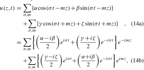
be understood from following the example of wave superpo-sition illustrated by Eqs. (14a), (14b): Assume the perturba-tion velocityu(z,t )(so isv (z,t ))results from the superposi-tion of phase-upward propagating waves (1st term of r.h.s. of Eq. 14a) and phase-downward propagating waves (2nd term of r.h.s. of Eq. 14a),

u(z,t )=X

σ,m

{αcos(σ t−mz)+βsin(σ t−mz)}

+X

σ,m

{γcos(σ t+mz)+ζsin(σ t+mz)} , (14a)

=X

σ,m

_α−iβ

2

eiσ t+

_γ+iζ

2

e−iσ t

e−imz

+X

σ,m

γ−iζ

2

eiσ t+

α+iβ

2

e−iσ t

eimz, (14b) where coefficients α, β, γ and ζ are real functions of σ and m. Evidently, the complex coefficients of e−iσ t in Eq. (14b) cannot vanish simultaneously, therefore, it is im-possible to separate upward waves from downward waves by single Fourier transform over height (or time) as rotary spec-tra method did.

In contrast to the rotary spectra method, the separation of upward and downward waves in phase and group veloc-ity tracing technique involves double Fourier transform over height and time (see Sect. III-1 of Kuo et al., 2003). It does completely separate phase-upward propagating waves from phase-downward propagating waves, but does only partially separate waves with upward group velocity and waves with downward group velocity due to the Doppler effect. If the background wind is negligible, the intrinsic frequencyωwill be equal to the observed frequencyσ(σandmare positively defined in Eq. 14b), then the group velocities and phase ve-locities of all the wave packets will have opposite sense of vertical propagation (to be referred as type 1 wave packets). If the background wind is not negligible, some waves may be Doppler shifted into negative intrinsic frequency (see Eq. 1a) causing their vertical group velocities and phase velocities to have the same sense of vertical propagation, and we called such wave packets as type 2 wave packets (Kuo et al., 2003, 2008, 2009; Kuo and R¨ottger, 2005). Phase and group ve-locity tracing technique can unambiguously identify the lo-cation (height and time) of type 1 and type 2 wave packets. Among previous wave packet researches, about 85 % were type 1 while 15 % were type 2 wave packets in one study of SOUSY-Svalbard Radar observation (Kuo et al., 2003); and about 76 % were type 1 while 24 % were type 2 wave pack-ets in another study of SOUSY-Svalbard Radar observation (Kuo and R¨ottger, 2005). In a recent study of the MU Radar observation (Kuo et al., 2008), only 6 % were type 2 wave packets and 94 % were type 1 packets. These statistics re-vealed that type 2 wave packets represented approximately less than 25 % of the gravity wave packets.

Phase and group velocity tracing technique offers three de-terminations: observed wave period, vertical phase velocity

48   

5 

Fig.9 A partial range-time plot of

( )

10 

observed by the MU radar at Shigaraki Japan on November 15 in 1988. Measurement

of vertical phase and group velocities of wave packets were indicated by the phase lines

(along the patch) and energy lines (across the patch).

15 

Time (min)

H

e

ight

(

K

m

)

550 600 650 700 750 800 850

72 74 76 78 80 82 84 86 88 90

1 2 3 4 5 6 7 8 9 10

Fig. 9. A partial range-time plot of(δV )2of meridional velocity converted from dataset observed by the MU radar at Shigaraki Japan on 15 November 1988. Determination of vertical phase and group velocities of wave packets were indicated by the phase lines (along the patch) and energy lines (across the patch).

and vertical group velocity. From these three determinations observed frequency σ, vertical wavelength λz, along with vertical group velocity vgz are readily obtained. Then the intrinsic frequencyω, horizontal wavelengthλhand azimuth φaz(if the background wind velocity is known) can be ob-tained by fitting the three determinations into Doppler rela-tion and dispersion Eqs. (1a), (1b) and its related Eq. (10) for vertical group velocity. In such a manner, the derived quantities ω, λh and azimuth φaz were forced to satisfy Doppler relation and dispersion Eqs. (1a), (1b) and its related Eq. (10), but were not forced to satisfy polarization relation. By contrast, Stokes parameters/rotary spectrum method also offers three determinations following polarization relation: ω, λz and φaz. Then λh can be obtained from dispersion Eq. (1b). However, these parameters were not forced to sat-isfy Eqs. (1a) and (10). Evidently, these two methods are complementary to each other, and it may be worth develop-ing a composite method of wave packet analysis combindevelop-ing these two methods.

5 An example of composite wave packet analysis of real radar data

568 H. Y. Lue and F. S. Kuo: Comparative studies of methods of obtaining AGW’s propagation properties

this dataset was 9 AM–3 PM with time resolution of 147 s; and the height range was 63.6–99.3 km with height resolu-tion of 300 m. The constant mean wind velocity had a mag-nitude of 30.97 m s−1 with an azimuth angle of 65.54◦. A time window of 30 min–3 h (2nd to 12th frequency mode) and wavelength window of 5.95 km to 35.7 km (1st to 6th wave number mode) to separate upward phase velocity waves from downward phase velocity waves.

The vertical phase velocity, vertical group velocity and characteristic wave period of the wave packet in Fig. 9 de-termined by phase and group velocity tracing technique were τ=69 min, vpz=1.917 m s−1 andvgz= −0.831 m s−1, re-spectively. The vertical wavelengthλz=7.94 km was read-ily obtained. Substituting these values into Doppler relation and dispersion equations and its derived group velocity equa-tions, we obtained the characteristic intrinsic period, hori-zontal wavelength and azimuth angle as follows:τ=2.51 h, λh=236.1 km andφaz=60.9◦or 69.9◦, with relative error of vertical group velocity vgz− ˜vgzvgz

=0.01 and phase

velocity vpz− ˜vpzvpz

=0.01, satisfying condition (9).

The uncertainty of azimuth angles (φaz=60.9◦or 69.9◦) can be solved with the help of Stokes parameters analysis. First of all, we noticed that phase and group velocity tech-nique tends to yield wave parameters corresponding to high frequency part of the wave packet’s component waves, while Stokes parameters analysis tends to yield a result correspond-ing to a low frequency part of the wave packet’s compo-nent waves. So we use a time window of 30 min to 1 h (6th to 12th frequency mode) and wavelength window of 5.95 km to 35.7 km (1st to 6th wave number mode, same as the window for velocity tracing analysis) to separate upward phase velocity waves from downward phase velocity waves. Then we applied spectra method of Stokes parameters anal-ysis to calculate Stokes parameters from Eqs. (12a)–(12d) using the 4th wave number mode (m=4, corresponding to 8.925 km of vertical wavelength), and taking time average over a time range of 138 min (corresponding to 2 periods time of the wave packet) with its time centre right at the time centre of the wave packet (756.5 min) in Fig. 9. We finally obtained intrinsic wave periodτ=1.69 hr and azimuth an-gleφaz=74.1◦orφaz=254.1◦. Comparing with the result of phase and group velocity tracing technique (τ=2.51 h, λh=236.1 km and φaz=60.9◦ or 69.9◦), the intrinsic pe-riods were reasonably close to each other and we decided that the azimuth of the wave packet was 69.9◦. So the pro-jection horizontal wavelength along the north-south line was 687 km, which was long enough to make the error in merid-ional wind measurement (by dual beam method) negligible. Here we would like to emphasize that we had used differ-ent combinations of the range of vertical wave numbers for mode summation and the range of time for time average to calculate Stokes parameters, and the result above was closest to the result of velocity tracing technique. Detailed results of the study of mesospheric data observed by the MU radar will be presented in a separate paper (Kuo et al., 2012).

6 Summary

We may briefly summarize the results of the simulation stud-ies as follows. For the case of one monochromatic wave, hodograph analysis was perfect to obtain both the wave pe-riod and its propagation direction; Stokes parameters method was accurate to estimate the period and azimuth irrespec-tive of its vertical sense of propagation, but could not dis-tinguish between azimuthsφaz andφaz±180◦. The 180◦ -ambiguity can be solved by correlation with simultaneous measurements of temperature oscillations due to the polar-ization between temperature, zonal and meridional wind. In the case of two waves with same wave periods and wave-lengths, but different amplitudes propagating in opposite ver-tical direction, the hodograph would be perfectly fitted by an ellipse and revealed the same sense of vertical propagation of the major wave even when the amplitude ratio of minor to major wave was as large as 0.8. But the resulting wave period and azimuth from hodograph analysis was unaccept-ably erratic even when the amplitude ratio of minor to major wave was as small as 0.25. Stokes parameters method would yield the wave period larger than the original period, and the resulting azimuth was close (but not equal) to the weighting average of their azimuth angles. So separation of data into sets of upward propagating waves and downward propagat-ing waves before dopropagat-ing analysis is essential for hodograph analysis. Then we studied the simulation data in which all component waves propagated in the same vertical direction. For the case of superposition of 5 waves of different periods, wavelengths and azimuths as listed in Table 2a, the phase and group velocity tracing technique yielded that character-istic wave period, vertical wavelength and horizontal wave-length were all closely associated with the higher frequency part among the component waves. Though hodograph anal-ysis failed to yield reasonable result, its counterpart, Stokes parameters method, did yield reasonable period and azimuth if the spreading in azimuths of all component waves did not exceed 90◦, or more specifically, the resulting period would be larger than the period of the lowest frequency component wave, and the resulting azimuth would be dominated by the lowest frequency component wave. If all five waves in Ta-ble 2a propagated in the same direction vertically and hori-zontally, then all the three methods were meaningful: The re-sulting azimuth from hodograph method and Stokes param-eters method were consistent with the original waves, and their resulting periods tended to correspond to the low fre-quency part among the component waves, while the result from the phase and group velocity tracing technique tended to correspond to high frequency part among the component waves.

As a conclusion, we suggest that separation of upward propagating waves from downward propagating waves has to be made, and upward data and downward data must be treated independently. Then, Stokes parameters method would yield the characteristic intrinsic wave period, vertical

H. Y. Lue and F. S. Kuo: Comparative studies of methods of obtaining AGW’s propagation properties 569

wavelength and azimuth angle following polarization rela-tion; phase and group velocity tracing would identify the locations of wave packets and determine their characteristic wave period, vertical phase and group velocities, then hori-zontal wavelength and azimuth could be estimated from dis-persion equation and its related formula for vertical group velocity. However, if the continuous data record is too short, up-down separation process (see Sect. III-1 of Kuo et al., 2003) might give rise to serious error due to border effect and poor frequency resolution, then phase and group veloc-ity tracing technique might be less credible.

In case upward waves and downward waves cannot be ef-fectively separated, Stokes parameters method may remain the only effective method in determining gravity wave pa-rameters due to its insensitivity to the vertical sense of propa-gation. Conventionally, wavelet analysis was applied to iden-tify the location and the dominant scale of wave event, then narrow band filter was applied to pick out a specific signal for hodograph analysis and Stokes parameters analysis (Sato and Yamada, 1994; Serafimovich et al., 2005; Hoffmann et al., 2006; Chagnon and Gray, 2008).

For a gravity wave packet, phase and group velocity trac-ing technique will yield characteristic wave parameters cor-responding to the high frequency part of the wave packet; while Stokes parameters method will give characteristic wave parameters corresponding to the low frequency part. Phase and group velocity tracing technique follows disper-sion equation and its related formula, while spectra method of Stokes parameters analysis follows polarization relation. It is fair to say that these two methods are complementary to each other. However, the existence of type 2 wave pack-ets propagating in the wind field would cause some trou-ble in measuring upward/downward ratio of energy trans-ported by gravity wave. Phase and group velocity tracing is able to identify their locations for proper treatment, while Stokes parameters method does not have this merit. Phase and group velocity tracing technique and dispersion equa-tion would yield two azimuth angles symmetric with respect to the mean wind direction. This ambiguity of azimuth can be solved with the help of the spectra method of Stokes pa-rameters analysis as demonstrated in this paper.

Acknowledgements. This work is supported in part by the National Science Council of Taiwan under the contract number NSC 99-2111-M-238-001. We deeply thank the anonymous referees for their invaluable comments on this manuscript.

Topical Editor C. Jacobi thanks three anonymous referees for their help in evaluating this paper.

References

Chagnon, J. M., and Gray, S. L.: Analysis of convectively-generated gravity waves in mesoscale model simulations and wind-profiler observations, Q. J. Roy. Meteorol. Soc. 134, 663–676, 2008. Eckermann, S. D.: Hodographic analysis of gravity waves:

Re-lationships among Stokes parameters, rotary spectra and cross-spectral methods, J. Geophys. Res., 101, 19169–19174, 1996. Eckermann, S. D. and Vincent, R. A.: Falling sphere observations of

anisotropic gravity wave motions in the upper stratosphere over Australia, Pure Appl. Geophys., 130, 509–532, 1989.

Fritts, D. C. and Alexander, M. J.: Gravity wave dynamics and effects in the middle atmosphere, Rev. Geophys., 41, 1003, doi:10.1029/2001RG000106, 2003.

Gossard, E. E. and Hooke, W. H.: Waves in the Atmosphere, Else-vier, New York, p. 98, 1975.

Hamilton, K.: Climatological statistics of stratospheric inertia-gravity waves deduced from historical rocketsonde wind and temperature data, J. Geophys. Res., 96, 20831–20839, 1991. Hirota, I. and Niki, T.: A statistical study of inertial-gravity waves

in the middle atmosphere, J. Meteorol. Soc. Jpn., 63, 1055–1066, 1985.

Hoffmann, P., Serafimovich, A., Peters, D., Dalin, P., Goldberg, R., and Latteck, R.: Inertia gravity waves in the upper tropo-sphere during the MaCWAVE winter campaign – Part I: Obser-vations with collocated radars, Ann. Geophys., 24, 2851–2862, doi:10.5194/angeo-24-2851-2006, 2006.

Kitamura, Y. and Hirota, I.: Small-scale disturbances in the lower stratosphere revealed by daily rawin sonde observations, J. Me-teorol. SOC. Japan, 67, 817–831, 1989.

Kuo, F. S. and R¨ottger, J.: Horizontal wavelength of gravity wave in the lower atmosphere measured by the SOUSY Svalbard Radar, Chinese Journal of Physics, 43, 464–480, 2005.

Kuo, F. S., R¨ottger, J., and Lue, H. Y.: Propagation of gravity wave packets in the lower atmosphere observed by the SOUSY-Svalbard radar, Chinese Journal of Physics, 41, 309–325, 2003. Kuo, F. S., Lue, H. Y., Fern, C. L., R¨ottger, J., Fukao, S., and

Ya-mamoto, M.: Studies of vertical fluxes of horizontal momentum in the lower atmosphere using the MU-radar, Ann. Geophys., 26, 3765–3781, doi:10.5194/angeo-26-3765-2008, 2008.

Kuo, F. S., Lue, H. Y., Fern, C. L., R¨ottger, J., Fukao, S., and Yamamoto, M.: Statistical characteristics of AGW wave packet propagation in the lower atmosphere observed by the MU radar, Ann. Geophys., 27, 3737–3753, doi:10.5194/angeo-27-3737-2009, 2009.

Kuo, F. S., Lue, H. Y., Fukao, S., and Nakamura, T.: Studies of gravity wave propagation in the mesosphere observed by MU radar, in preparation, 2012.

Nakamura, T., Tsuda, T., Yamamoto, M., Fukao, S., and Kato, S.: Characteristics of gravity waves in the mesosphere observed with the middle and upper atmosphere radar, 2, Propagation direction, J. Geophys. Res., 98, 8911–8923, 1993.

Sato, K. and Yamada, M.: Vertical structure of atmospheric gravity waves revealed by the wavelet analysis, J. Geophys. Res., 99, 20623–20631, 1994.

570 H. Y. Lue and F. S. Kuo: Comparative studies of methods of obtaining AGW’s propagation properties

Tsuda, T., Kato, S., Yokoi, T., Inoue, T., Yamamoto, M., VanZandt, T. E., Fukao, S., and Sato, T.: Gravity waves in the mesosphere observed with the middle and upper atmosphere radar, Radio Sci., 26, 1005–1018, 1990.

Vincent, R. A. and Fritts, D. C.: A climatology of gravity wave mo-tions in the mesopause region at Adelaide, Australia, J. Atmos. Sci., 44, 748–760, 1987.