performance for predicting carbon dynamics in
terrestrial vegetation models
Verónika Ceballos-Núñez1, Andrew D. Richardson2,3,4, and Carlos A. Sierra1
1Max Planck Institute for Biogeochemistry, Hans-Knöll-Str. 10, 07745 Jena, Germany
2Department of Organismic and Evolutionary Biology, Harvard University, Cambridge, MA 02138, USA 3School of Informatics, Computing and Cyber Systems, Northern Arizona University, Flagstaff, AZ 86011, USA 4Center for Ecosystem Science and Society, Northern Arizona University, Flagstaff, AZ 86011, USA
Correspondence:Carlos A. Sierra ([email protected]) Received: 18 July 2017 – Discussion started: 9 August 2017
Revised: 1 February 2018 – Accepted: 15 February 2018 – Published: 16 March 2018
Abstract.The global carbon cycle is strongly controlled by the source/sink strength of vegetation as well as the capacity of terrestrial ecosystems to retain this carbon. These dynam-ics, as well as processes such as the mixing of old and newly fixed carbon, have been studied using ecosystem models, but different assumptions regarding the carbon allocation strate-gies and other model structures may result in highly diver-gent model predictions. We assessed the influence of three different carbon allocation schemes on the C cycling in veg-etation. First, we described each model with a set of ordinary differential equations. Second, we used published measure-ments of ecosystem C compartmeasure-ments from the Harvard Forest Environmental Measurement Site to find suitable parameters for the different model structures. And third, we calculated C stocks, release fluxes, radiocarbon values (based on the bomb spike), ages, and transit times. We obtained model simula-tions in accordance with the available data, but the time se-ries of C in foliage and wood need to be complemented with other ecosystem compartments in order to reduce the high parameter collinearity that we observed, and reduce model equifinality. Although the simulated C stocks in ecosystem compartments were similar, the different model structures re-sulted in very different predictions of age and transit time distributions. In particular, the inclusion of two storage com-partments resulted in the prediction of a system mean age that was 12–20 years older than in the models with one or no storage compartments. The age of carbon in the wood com-partment of this model was also distributed towards older
ages, whereas fast cycling compartments had an age distri-bution that did not exceed 5 years. As expected, models with C distributed towards older ages also had longer transit times. These results suggest that ages and transit times, which can be indirectly measured using isotope tracers, serve as impor-tant diagnostics of model structure and could largely help to reduce uncertainties in model predictions. Furthermore, by considering age and transit times of C in vegetation compart-ments as distributions, not only their mean values, we ob-tain additional insights into the temporal dynamics of carbon use, storage, and allocation to plant parts, which not only de-pends on the rate at which this C is transferred in and out of the compartments but also on the stochastic nature of the process itself.
1 Introduction
ca-pacity to store this carbon for long periods of time (Körner, 2017).
The C storage capacity of an ecosystem is determined by the collective behavior of vegetation compartments such as foliage, wood, and roots, which may also act as C sources and sinks among each other (Xia et al., 2013; Luo et al., 2017). The capacity of a vegetation compartment to oscillate between C source and sink has important implications for ecosystems in their response to perturbations and environ-mental change, i.e., their resilience. Carbon fixed during pho-tosynthesis is transported from the leaves (sources) to other parts of the plant (sinks). One of these sinks is the labile or non-structural carbon (NSC; Hartmann and Trumbore, 2016; Trumbore et al., 2015; Martínez-Vilalta et al., 2016), which may turn into a C source during critical events such as the start of the growing season (after periods of limited photo-synthesis; Richardson et al., 2013) and the recovery from disturbances such as drought (Hartmann et al., 2013), cold temperatures (Hoch and Körner, 2003), pollution (Grulke et al., 2001), or nutrient stress (Ericsson et al., 1996). De-spite the importance of the source/sink capacity of NSC re-serves, many questions remain unsolved. For example, are NSCs completely depleted when needed, and replenished af-terwards? Is the C that has remained stored for many years still available for the plant? (Richardson et al., 2013).
It is indeed possible that the carbon stored in vegetation compartments, including NSCs, has been fixed at different times, resulting in a mix of ages (Muhr et al., 2016). Stud-ies across wood rings in temperate forest trees revealed that the mean age of NSCs in stemwood can be up to several decades old (Richardson et al., 2013; Trumbore et al., 2015). Trumbore et al. (2015) explained these old ages with a sim-ple model consisting of one NSC compartment with inward mixing of younger and older C. Alternatively, Richardson et al. (2013) proposed a model with two separate NSC stor-age compartments – with old and young C – that exchange material among each other. It is therefore uncertain how this mixing of NSCs of different ages occurs: either in the form of one single compartment in which all ages are mixed or in different compartments with separate ages.
Previous studies have focused mostly on determining ages of NSCs using radiocarbon-derived mean residence times, but this approach has limitations. One limitation is the am-biguity in the term “mean residence time”, which has been defined in different ways across studies; in some cases it im-plies the mean age of C in an ecosystem or ecosystem com-partment and in other cases it implies the time it takes C molecules to leave the system of compartments (Sierra et al., 2017). Another limitation is the use of mean values instead of complete frequency or density distributions to assess the spread of C ages in vegetation compartments.
The study of C age distribution in vegetation requires chal-lenging empirical methods, but can also be approached using ecosystem C cycle models. However, not all of the mod-els perform equally well because the assumptions behind
their structures may result in highly divergent predictions (Lacointe, 2000; Friedlingstein et al., 2006; Friend et al., 2014; Schiestl-Aalto et al., 2015). The performance of such models has been diagnosed by comparing their predicted C storage capacity and residence times (Friend et al., 2014; Yizhao et al., 2015), but if the abovementioned ambiguities are resolved, ages of carbon in vegetation and in respira-tion fluxes can serve as excellent addirespira-tional diagnostics of ecosystem models, and can give important insights into car-bon metabolism in vegetation under stress conditions, such as in the case of drought stress.
1.1 Definitions of ages and transit times
CO2molecules are fixed continuously by photosynthesis
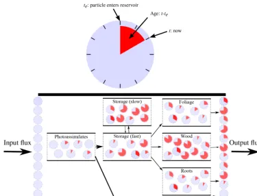
dur-ing the growdur-ing season; so, C particles enter the vegeta-tion (from here on called “system”) at different times during the year. After fixation, the photosynthetic products transit through the vegetation compartments until they eventually leave the system, either as CO2back to the atmosphere or as
litter and exudates to the soil. This means that at a given time (t) each particle in the system has a differentage, which is the time that it has remained within the system since its fixa-tion from the atmosphere. The time that each particle spends transiting through the system, from arrival until exit, is called transit time(Bolin and Rodhe, 1973).
At each time step, a particle may stay where it is, given by a certain probability, or flow to the next compartment with a rate or probability given by the transfer coefficients (also know as cycling rates). This means that the age of carbon in a system results from stochastic and deterministic processes, which are illustrated in Fig. 1; given two organic molecules in a compartment, one that has remained in the system for longer time than the other, they both have the same probabil-ity to either leave the system or move on to another compart-ment. Thus, if by chance older molecules remain for longer times, then the system’s age gets older. But the pace at which these molecules are transiting is moderated by the cycling rates. This is why slow cycling compartments have older C.
Lets describe a system of well-mixed C (distributed in multiple compartments) with the system of ordinary differ-ential equations
˙
x(t )=B×x(t )+β·u, x(0)=x0,
Figure 1.Graphical representation of the concepts of age and transit time distributions in a vegetation model. Carbon particles are represented here as clocks that measure the time they have been in the system. “System age” can be defined as the age of all particles in the system at a given time, while “transit time” as the age of particles in the output flux. Adapted from Sierra et al. (2017).
Given that each particle in the system has its own age and transit time, the age and transit time of the whole system can be considered as random variables. Additionally, the age and transit time of particles in a system’s compartment is expo-nentially distributed. Then, the age and transit time distribu-tions of the entire system would be the sum of those expo-nential distributions, i.e., a phase-type distribution (Metzler and Sierra, 2018).
The calculation of how many C particles have a certain age, or the age density distribution of a system(fA(y)), is
determined by the probability of entering the system through a given compartment and the rates at which C is transferred from one compartment to another until it leaves the system. Consistent with the symbols from the previous equation
fA(y)=zT ·ey·B·
x∗
||x∗||. (2) fA(y)is a function of (i) how fast the carbon is leaving the
system: the row vector of release rates, which is the column-wise sum of the elements of the B matrix (zT = −1TB); (ii) the transition probability matrix (eyB); and (iii) the rel-ative amount of C stock at steady state with respect to the total(||xx∗∗||). Notice that we use here the symbol|| · ||to rep-resent the vector norm, which is the sum of all entries of the vector.
The mean age is given by the expected value (E[A])
E[A] =
||B−1×x∗||
||x∗|| . (3)
Likewise, the transit time density distribution (fFTT(t )) is
also a function ofzT and the transition probability matrix (etB), as well as the vector of input distributions (β).
fFTT(t )=zT·et·B·β. (4)
The mean transit time is defined asE[FTT]:
E[FTT] = ||B−1×β|| =
||x∗||
||u||. (5)
From these equations it is evident that age and transit time calculations mainly depend on the schemes of C partition-ing (β) and cyclpartition-ing (B) within a vegetation model. There-fore, if we want to understand processes such as the mixing of old and newly fixed NSC using ecosystem models, it is critical to model proper carbon allocation (CA) strategies. Unfortunately, it is still uncertain what assumptions and sim-plifications should be done. How many carbon compartments are necessary to describe carbon cycling in vegetation? How are these compartments interconnected and how fast are they transferring C among each other? These are important ques-tions that need to be addressed to improve our understanding of vegetation dynamics, and predict consequences of envi-ronmental change on vegetation.
In this contribution, we address the following question: how do different C allocation schemes affect the ages and transit times of carbon in vegetation models? In particular, we are interested in understanding whether different car-bon allocation strategies would lead to different patterns of mixing of ages for the NSC compartment. For this work, we implemented three carbon allocation schemes based on Richardson et al. (2013); the models have either no stor-age, one storage compartment, or two storage compartments (fast and slow C cycling). Our approach is mostly theoreti-cal, and we are mainly interested in introducing the concepts of age and transit time distributions as useful model diag-nostics as well as an approach to explain mixes of C age in NSC compartments. For this purpose, we used published measurements on ecosystem C compartments from the Har-vard Forest Environmental Measurement Site to find suitable parameter values for the different model structures. We also diagnosed the performance of these models using as metrics (1) C release fluxes (respiration and other carbon losses such as litterfall), (2) the dynamics of radiocarbon (based on the bomb spike) for individual compartments, (3) the transit time distribution of the system, and (4) the age distribution of C in the system and in each compartment.
2 Methods
2.1 Model implementation
Each model was written as a set of ordinary differential equa-tions (based on Eq. 1) within the environment of the R pack-ageSoilR(Sierra et al., 2012). All models met the require-ments of Eq. (1); they are autonomous (their dynamics do not depend on variables that change with time) linear sys-tems with multiple interconnected compartments. The initial carbon stocks, and some of the parameter values needed to solve those equations, were obtained from the literature, from a deciduous–evergreen model with similar carbon allocation schemes (Fox et al., 2009). Other parameter values were ob-tained from an optimization procedure (see below).
As means to assess whether the carbon allocation strate-gies had an impact on the mixing of C age in vegetation com-partments, we implemented three models whose carbon allo-cation strategies varied depending on the number of storage compartments (0, 1, or 2; Fig. 2), following the hypotheses proposed by Richardson et al. (2013). Given that we aimed at a theoretical comparison of the abovementioned strategies, we eliminated other potential sources of variation that may act as confounding factors by assuming that all C transfers between the compartments depended on constant rates. We also assumed that there was a constant photosynthetic input – gross primary production (GPP):u– of 1400 g C m−2year−1 (Urbanski et al., 2007). Environmental variability, which op-erate mostly on hourly to daily timescales, was not consid-ered here because we ran the models at an annual timescale; i.e., without diurnal cycles or phenology.
Fixed photosynthetic input enters the system through the “Photoassimilates” compartment, and part of the carbon is released back to the atmosphere at each time step, in a flux proportional to the size of Photoassimilates and the constant rate Ra (Fig. 2). In the model without a storage
compart-ment, the C stored in the Photoassimilates is partitioned into “Structural Foliage” (from here on Str. Foliage), Wood (in-cluding branches and coarse roots), and Fine Roots (from here on Roots), with the constant ratesAf,Aw, andAr; part
of the C stored in these three compartments also leaves the system with constant ratesLf,Lw, andLr, which comprise
all the carbon released through respiration and other losses (e.g., litterfall). For the models with storage, the C is trans-ferred from the Photoassimilates to the fast cycling storage, from which it is then partitioned to the rest of the compart-ments. In addition to the fast cycling storage, the model with two storage compartments also has a slow cycling compart-ment.
2.2 Optimization procedures
To obtain results that can be related to a particular ecosys-tem, we performed a parameter estimation procedure us-ing published measurements of two ecosystem C compart-ments from the Harvard Forest Environmental Measurement Site (see footnote links1 and for the raw leaf area index, LAI2). Harvard Forest is a regenerating temperate forest located in Petersham, Massachusetts (42.54◦N, 72.18◦W; 340 m a.s.l.). Among the tree species that are found in this 65 to 85 year-old mixed deciduous forest are red oak, red maple, white and red pine, yellow and white birch, beech, ash, sugar maple, and hemlock (Wofsy et al., 1993).
We calculated C stocks in wood and foliage from the abovementioned aboveground biomass, LAI, and leaf mass
1http://atmos.seas.harvard.edu/lab/hf/index.html,
http://ameriflux.lbl.gov/doi/AmeriFlux/US-Ha1, http://ameriflux.lbl.gov/sites/siteinfo/US-Ha1
2http://ftp.as.harvard.edu/pub/nigec/HU_Wofsy/hf_data/
Figure 2.Three carbon allocation strategies in vegetation models. These strategies differ in the number of storage compartments, Storage: 0, Storage: 1, and Storage: 2. Adapted from Richardson et al. (2013). The parameters are the rates at which the carbon cycles into and out of the compartments; thus, the fluxes are proportional to the C stocks and the rates. Notice that the foliage is divided into two compartments: Photoassimilates and Structural Foliage.
per area (LMA), using allometric equations. Although in pre-vious studies, performed at the same site, the use of woody biomass increment and LAI reduced the uncertainties in the predictions of net C sequestration and foliage dynamics, re-spectively (Keenan et al., 2013), and the wood stock observa-tions have been used to successfully constrain fine root mass simulations (Smallman et al., 2017), we obtained unrealis-tic simulations of C stocks in storage and roots because these pools were not well constrained. Thus, we estimated C stocks of roots based on the assumption that shoot to root ratio is 1 :5, and we also used published ratios to calculate NSC from Wood carbon (p. 5 of Richardson et al., 2010).
We were also interested in observing the uncertainty in the model simulations (see section below), so we performed a Bayesian optimization, which gave us alternative parame-ter sets afparame-ter exploring the parameparame-ter space. This optimiza-tion procedure was started using the result of a classical op-timization method using the R package FME (Soetaert and Petzoldt, 2010). Taking into account that data uncertainties have a direct influence on the fit of the outcome of the pa-rameter estimation (Richardson et al., 2010), we accounted for the uncertainty in the data using the standard deviation of the measurements in the cost functions.
As means to evaluate whether the parameters could be esti-mated from the given data sets, i.e., parameter identifiability, we performed a local sensitivity analysis and estimated the collinearity of the parameter sets with the packageFME. The obtained collinearity indexγ expresses the degree at which pairs of parameters are linearly related. Values ofγ >20 in-dicate high collinearity among parameters and poor identi-fiability of the model given the available data (Soetaert and Petzoldt, 2010).
Given the high correlation between some of the parame-ters, we decided to run all model simulations using the pa-rameter set that was most frequently chosen by the Bayesian optimization method. We then calculated C stocks, release fluxes, radiocarbon values based on the bomb spike, ages,
and transit times, using functions implemented in SoilR. The functions that calculate age and transit time distributions are based on the formulas proposed by Metzler and Sierra (2018).
2.3 Uncertainty analysis
In order to explore model predictions that could result from different parameter sets that were possible and likely, we ex-tracted a random sample of 1000 posterior parameter sets from the Bayesian optimization that used Markov chain Monte Carlo. We ran the models with the unique sets, and calculated the weighted mean and standard deviation of the C stocks, the released C from each compartment, and the sys-tem’s mean age and transit time. The weights corresponded to the number of times that each parameter set was repeated in the sample.
3 Results
3.1 Simulations of carbon stocks
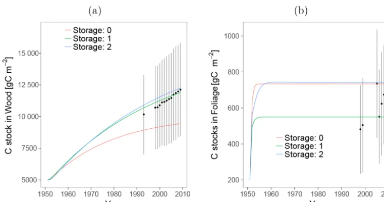
The C stock simulations obtained from the three models were within the uncertainty range of the available data (Figs. 3 and 4). The simulations of Wood and Foliage C (Photoassimi-lates+Structural) stocks were in accordance with the stocks estimated from the aboveground biomass inventory data and the LAI, respectively.
All of these predictions were obtained using the parameter set that was most frequently chosen by the Bayesian opti-mization method (Table 1). This table also shows two quan-tiles of the distribution of each parameter value after explor-ing the parameter space.
Figure 3.Carbon stocks estimated for each model, comparing the observed data and the model predictions of C stocks in Wood(a)and Foliage(b).
Table 1.Parameter values obtained from the optimization procedures (year−1).
Model Parameter Final Best1 Best2 Median q25 q75
Storage: 0 Ra 0.64 0.7 0.7 0.57 0.45 0.64
Af 0.48 0.5 0.5 0.42 0.32 0.46
Ar 0.32 0.5 0.5 0.33 0.26 0.4
Aw 0.5 0.49 0.49 0.47 0.43 0.49
Lf 35.09 17.84 17.84 32.12 28.47 34.92
Lr 0.06 0.12 0.12 0.09 0.07 0.1
Lw 0.04 0.02 0.02 0.03 0.03 0.04
Storage: 1 Ra 0.61 0.32 0.32 0.52 0.35 0.61
Af 0.31 0.17 0.17 0.19 0.13 0.3
Ar 0.47 0.5 0.5 0.36 0.3 0.43
Aw 0.29 0.3 0.3 0.37 0.32 0.44
Lf 3.04 7.9 7.9 10.82 6.49 14.18
Lr 0.13 0.21 0.21 0.17 0.14 0.19
Lw 0.02 0.03 0.03 0.04 0.03 0.05
As 2.55 2.14 2.14 3.55 2.26 4.29
Storage: 2 Ra 0.65 0.7 0.7 0.58 0.5 0.65
Af 0.15 0.1 0.1 0.16 0.14 0.18
Ar 0.47 0.5 0.5 0.44 0.39 0.47
Aw 0.23 0.19 0.19 0.23 0.21 0.28
Lf 0.74 17.52 17.52 17.89 12.03 21.6
Lr 0.23 0.21 0.21 0.27 0.23 0.35
Lw 0.02 0.01 0.01 0.02 0.02 0.03
As 2.27 1.69 1.69 1.96 1.67 2.26
As12 2.77×10⁻³ 1.00×10⁻³ 1.00×10⁻³ 1.83×10⁻³ 1.43×10⁻³ 2.16×10⁻³
As21 0.09 0.82 0.82 0.41 0.22 0.60
Final: parameter set that was most frequently chosen by the Bayesian optimization method and was used for all of the simulations, unless otherwise noted. Best1: parameter set obtained from the classical optimization procedure.
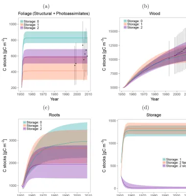
[image:6.612.76.521.367.681.2]Figure 4.Carbon stocks estimated for each compartment and their uncertainties. Carbon in the(a)Foliage (Photoassimilates+Structural),
(b)Wood,(c)Roots, and(d)storage compartments.
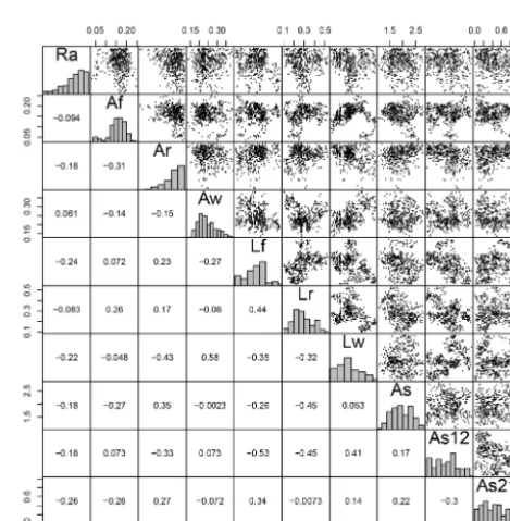
for the models Storage: 0, 1, and 2 was 3, 4, and 5, respec-tively. The correlations can be seen in the pairwise plots of sensitivity functions (Figs. A1–A3). Table A1 summarizes the number of parameter correlations that we observed under the diagonal of the pairwise plots of sensitivity functions. For this reason, the results presented here need to be interpreted within the context of predicted uncertainties.
3.2 Influence of carbon allocation strategies on ecosystem-level C cycling
To assess the impact of different carbon allocation strategies on the ecosystem C cycling, we used the following metrics: (1) C release fluxes, (2) dynamics of radiocarbon for individ-ual compartments, (3) transit time distribution of C through the system, and (4) age distribution of C in the system and in each compartment. The calculations required for these
met-rics were performed using the parameter set that was most frequently chosen by the Bayesian optimization method for each model, unless otherwise noted.
3.2.1 Fluxes of C released from the compartments
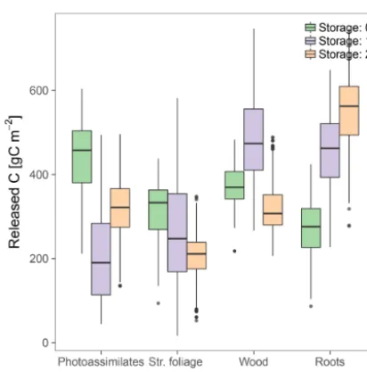
Figure 5.C release fluxes from the compartments at steady state, with uncertainty ranges obtained from the set of posterior parame-ters obtained by Bayesian optimization.
3.2.2 Radiocarbon content in each compartment The simulated radiocarbon content of fast cycling compart-ments (e.g., Photoassimilates, Str. Foliage, and Storage fast) had a stronger resemblance to the atmospheric114C values than the slower cycling compartments (Fig. 6). However, for the Str. Foliage of the models with storage there was a time lag of about 3–5 years with respect to the peak that corre-sponds to the “bomb spike”. Furthermore, the accumulation of radiocarbon in slow cycling compartments such as Wood and the Storage (slow), was characterized by a slow incor-poration of radiocarbon that resulted in large 114C values for the last part of the curve. The radiocarbon accumulation in the Roots compartment was not as fast as in the Foliage compartments, but was faster than that of the Wood.
Differences in radiocarbon values for the different com-partments hint to different levels of mixing of carbon fixed at different times. For the fast cycling compartments such as the Photoassimilates, the degree of mixing is relatively low because most of the radiocarbon reflects the values in the at-mosphere. For other compartments that cycle at slower rates, the mix of recent and old radiocarbon results in important divergences from the atmosphere. Mixing of carbon of dif-ferent ages can be further studied with ages and transit time distributions.
3.2.3 Age and transit time distributions
The age and transit time distributions were calculated assum-ing that the system was in steady state. These distributions had a wide range, expanding from zero to several decades old carbon, and their shape varied according to the model
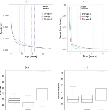
struc-ture (Fig. 7). The ascending order of the models according to their mean age, from young to old, was Storage: 0, Stor-age: 1, and StorStor-age: 2. As expected, the model with the oldest ages (Storage: 2) had the longest transit time. These trends were partially observed when we analyzed the uncertainties in mean age and mean transit times (Fig. 7c and d), but the uncertainties were large. These large uncertainties may have resulted from the high correlation between the model param-eters.
At the compartment level, the abovementioned age-dependent ranking of the models only holds true for Wood (Fig. 8), which was the compartment with the closest resem-blance to the overall system age densities because it com-prised most of the mass in the system. The inclusion of two storage compartments in Storage: 2 resulted in a relatively flat distribution; with a long tail that leads to a mean age 10– 20 years older than the other two models, but with a peak at very young ages. This contrasts with the other models, which peaked at around the same time, but had steeper declines with age.
The only compartment that had an age maximum at 0 years was the Photoassimilates. Hence, it had a unique distribution curve reflecting the fact that all new carbon (age=0 years) enters the models only through this compartment. Although the other fast cycling compartments (Str. Foliage and Roots) had peaks after 0 years, their C age was distributed towards young ages, with mean ages between 1 and 3 years. This spread in the C age of Str. Foliage for the models with storage may suggest either that the cycling rate of this compartment was relatively slow or that it received C from compartments with older carbon.
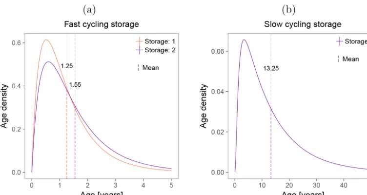
The age densities of the storage compartments, just as the ones for Foliage, Wood, and Roots, consisted of curves with peaks at young ages and long tails (Fig. 9). In the case of the fast cycling compartments, the mean ages of the models Storage: 1 and Storage: 2 were 1.25 and 1.55 years, respec-tively, but the long tail indicates that it is also probable to find 5 year-old C in this compartment. The mean age of the slow cycling compartment was 13.25 years, but the mixing of ages is also observed in the density curve where age of C ranged from 0 to more than 50 years.
4 Discussion
Figure 6.Radiocarbon simulations for the three model structures. The black curve corresponds to the114C in the atmosphere, and the other colors depict the vegetation compartments.
4.1 Diagnosing model performance with C release fluxes, and age and transit time distributions
The simulated ecosystem properties that were more strongly impacted by the assumptions behind model structure were (i) the fluxes of C released from each compartment and (ii) the ages and transit time distributions of carbon in the system and in each compartment. This sensitivity to different carbon allocation strategies makes them good candidates for diag-nosing model performance.
Given that the C release fluxes from Photoassimilates, Roots, and Wood were highly sensitive to the three model structures, empirical measurements of these compartments could be used as constraints during the parameter estimation procedure. Radiocarbon accumulation was less sensitive, but can be useful to diagnose the models’ performance accord-ing to the cyclaccord-ing speed of their compartments. As an exam-ple, we could identify the short delay of the114C signature of the Str. Foliage compartment with respect to the current
year’s atmosphere, in the models with storage (Fig. 6). Al-though such a delay could indicate that this compartment had a slightly slower C cycling than what is expected for a decid-uous forest (Trumbore et al., 2002, 2015), it could also indi-cate the flux of old C from the slow cycling compartments into the foliage. This delay in radiocarbon accumulation was also observed as shifts to older ages in the age distributions (Fig. 8), with a resolution of months. In general, radiocarbon measurements can also help to constrain model parameters with respect to how fast or slow different compartments cy-cle C (Trumbore et al., 2016), but with less resolution than the age and transit time distributions.
in-Figure 7.System ages and transit times.(a)Age and transit time(b)density distributions calculated for each model structure using the best parameter set from the optimization; the dashed and dotted lines mark the mean and median ages, respectively. Spread of mean ages(c)and mean transit times(d)obtained from all posterior parameter sets from the Bayesian optimization.
clusion of storage compartments had respectively direct and indirect effects on the predictions of the abovementioned dis-tributions.
On the one hand, as we initially inferred from Eqs. (2)–(5), the calculation of age and transit time distributions depends on the C partitioning schemes (β) and the transfer – cycling – rates between plant compartments (B). Therefore, different parameter values that compose the vectorβand matrixB di-rectly result in the different calculations of ages and transit time distributions. This was tested by running the three mod-els using the same parameter set; although they still differed in the number of storage compartments, there was almost no difference between the age and transit time distributions in the whole system and in the compartments (Figs. A6, A7, and A8). These similarities were also observed for the ra-diocarbon accumulation (Fig. A5). The only exceptions to
the above were the foliage compartments of the model Stor-age: 0, which were faster than in the other two models.
[image:10.612.114.487.70.448.2]Figure 8.Age densities simulated for the compartments:(a)Photoassimilates,(b)Str. Foliage,(c)Wood, and(d)Roots. Each model structure is depicted in a different color. Dashed lines correspond to mean ages.
As expected, systems with ages distributed towards older values also have older transit time distributions. In fact, their correlation can be confirmed by observing the formulas once again. The calculation of these two properties depends on the matrix of transfer coefficients (B), but there are other factors driving these two distributions. The additional factor driving the mean age calculation is the relative amount of C stock at steady state; whereas the mean transit times depend on the C partitioning schemes (β; Metzler and Sierra, 2018). So, the mean transit time calculation is only limited by the rates of C transfer, while the mean age of C in the system also depends on its mass. This is why the mean age of C in vege-tation is determined by the age of the compartment where the majority of the mass is stored, which in this case is Wood. We further explored this relation in the scatter plot in (Fig. A9), where the distribution of the points below the 1: 1 line
indi-cate that the three models have mean ages greater than their mean transit times. This means that they have large masses of old carbon, but they also have highly dynamic compartments through which carbon transits very fast.
Figure 9. Age densities simulated for the models with storage compartments. (a)Fast cycling compartment of models Storage: 1 and Storage: 2.(b)Slow cycling storage of the only model with two storage compartments.
compartments show that even though they are well mixed, their C do not have the same age. Thus, it is also likely to find C between 0–5 and 0–50 years in the fast and slow cycling storage compartments, respectively. This resonates with the fact that although stemwood NSC is highly dynamic on sea-sonal timescales, it can also be surprisingly old (Richardson et al., 2013). Then, the two hypotheses regarding C mixing – inward mixing of younger and older C in one compart-ment (Trumbore et al., 2015) and two compartcompart-ments (young and old) that mix (Richardson et al., 2013) – converge in the concept of age distributions because C is simultaneously been fixed and removed from the compartments at different times, a process that results in C age distributions. We can think about these dynamics in the context of a stochastic pro-cess. The total amount of C that enters and leaves each com-partment is fixed and given by the deterministic model, but the time that each C particle stays in a compartment varies stochastically within them. So, the age distribution of C par-ticles in each compartment is a mix of new and old carbon, with distribution functions emerging from the deterministic model (Eq. 2).
Another important observation regarding the mean age predictions is the fact that these calculations were performed under the assumption that the system, in this case the for-est, was in steady state. Since the C stocks in Harvard Forest continue growing, the calculated mean ages and transit times should be interpreted as predictions of the mean age that the carbon may have in this forest once it is in steady state. Based on this, the time that this forest will take to reach the steady state is highly divergent among the three models. As an ex-ample, the model with two storage compartments would pre-dict 20 years more of growth to reach a steady-state close to that of the model with no compartments.
In the case of systems that are driven by environmental variables and result in time dependencies of inputs (GPP) and process rates, the mean ages and transit time distribu-tions would also change over time. To calculate the means of these time-dependent distributions one would need to know the complete history of inputs and cycling rates for the dura-tion of the simuladura-tion (Rasmussen et al., 2016), informadura-tion that is not available for Harvard Forest. Nonetheless, we can predict that if there were external factors influencing the sim-ulations, there would be a different prediction of mean ages and transit times at each time step, but the model structure (C allocation scheme in particular) would play a major role determining the shape of these distributions.
ties in the parameter values can be reduced by constraining them with age and transit time distributions. These improved models could then be used to test hypotheses regarding phys-iological questions, and assess the sustainability of current terrestrial C sinks, given changes in environmental forcing. 4.2 Model equifinality (identifiability)
Model equifinality (Medlyn et al., 2005) was evident from the fact that despite having a different number of compart-ments and values of cycling rates, all three of the models had similar simulations of C stocks (Figs. 3 and 4). Along with model equifinality, we obtained a high collinearity between some parameters, implying that they are non-identifiable, i.e., they cannot be uniquely estimated from the given data sets (Soetaert and Petzoldt, 2010). Thus, for these particular mod-els, the time series measurements from only 2 out of 4–6 veg-etation compartments is not sufficient to estimate the values of 7–10 parameters.
Model equifinality as well as the impossibility to uniquely identify certain parameters (parameter non-identifiability) is expressed as high correlations between the parameter sets. Positive parameter correlations may indicate practical non-identifiability, where the insufficiency or poor quality of data is not a good constraint for the parameters. In addition, a neg-ative parameter correlation can be a symptom ofstructural non-identifiability, which is the result of a redundant param-eterization (Raue et al., 2009; Timmer, 2011; Raue et al., 2012; Cressie et al., 2009). Thus, the three models had practi-cal and structural non-identifiabilities, which means that they need to be constrained with more and better data, and they need to be restructured in order to avoid compensation of fluxes into and out of the compartments.
Since this study was limited by the availability of relevant empirical data, the parameter values that we used are only one of many possible outcomes of parameter estimations us-ing the same data sets. Therefore, it is possible that none of these models accurately depict the C cycle in the Harvard Forest. However, these problems experienced with parame-ter non-identifiability are not an isolated case; the process of finding unknown rates of C sequestration by fitting biosphere models to empirical data (Luo et al., 2003) is often hampered by parameter non-identifiability (Schaber and Klipp, 2011). This is a real problem because parameters such as those that
vegetation compartments results in C age distributions not explored in previous studies. The shape of these distributions depends largely on model structure, and in particular on how carbon allocation is represented in models.
Models with none or one storage compartment may fail to explain the mixing of ages found in different vegeta-tion compartments, but they are more parsimonious than the model with two storage compartments. Nonetheless, param-eter collinearity and model equifinality were persistent prob-lems that might be solved if more constraints are added, since the time series of C in foliage and wood are not enough to pa-rameterize a full vegetation model.
Although all models predicted similar C stocks in vege-tation compartments, the inclusion of a carbon storage com-partment resulted in very different predictions of age, transit time distributions, C release, and isotopic composition. Thus C ages and transit times, which can be indirectly measured using isotope tracers, can be used to improve biosphere mod-els via examination of their structure and estimation of pa-rameter values, which then can be used to assess the strength of C sources or sinks from vegetation.
Finally, it is advantageous to consider age and transit times as distributions, rather than only mean values; with their dis-tributions we obtain additional insights into the temporal dy-namics of carbon use, storage, and allocation, which not only depends on the rate at which C flows into and out of the com-partments but also on the stochastic nature of the process it-self.
Appendix A: Supplementary figures and tables
Figure A1. Pairwise plots of sensitivity functions for the model Storage: 0.
[image:14.612.310.545.256.496.2]Figure A2. Pairwise plots of sensitivity functions for the model Storage: 1.
[image:14.612.46.289.402.646.2]Figure A4.Carbon stocks estimated for each model, comparing the observed data and the model predictions of C stocks in Wood(a)and Foliage(b). The C stocks from models Storage: 1 and 2 overlap. The three models were run using the same parameter set.
[image:15.612.133.468.341.669.2]Figure A6.System ages and transit times.(a)Age and transit time(b)distributions calculated for each of the three models using the same parameter set; the dashed and dotted lines mark the mean and median ages, respectively. Some of the lines may be overlapping others.
[image:16.612.130.467.311.668.2]Figure A8.Age densities simulated for the models with storage compartments; the models were run using the same parameter set.(a)Fast cycling compartment of models Storage: 1 and Storage: 2.(b)Slow cycling storage of the only model with two storage compartments.
Figure A9.Scatter plot of mean age vs. mean transit times on a log scale. The three models have distributions below the 1:1 line.
Table A1.Number of positive and negative correlations between parameters. OnlyR2values<−0.1 and>0.1 were assumed to account for correlations.
Model Positive correlations Negative correlations Possible combinations
Storage: 0 05 09 21
Storage: 1 10 15 28
[image:17.612.139.455.639.695.2]The Supplement related to this article is available online at https://doi.org/10.5194/bg-15-1607-2018-supplement.
Competing interests. The authors declare that they have no conflict of interest.
Acknowledgements. Research at Harvard Forest is supported by the National Science Foundation’s LTER program (DEB-1237491). This material is based upon work supported by the US Department of Energy, Office of Science, Office of Biological and Environmen-tal Research. Part of this work was the result of a research visit to the Terrestrial Ecosystems and Global Change group, Department of Organismic and Evolutionary Biology, Harvard University. It was funded by the Max Planck Society and the German Research Foundation through its Emmy Noether Program (SI 1953/2–1).
The article processing charges for this open-access publication were covered by the Max Planck Society.
Edited by: Akihiko Ito
Reviewed by: four anonymous referees
References
Bolin, B. and Rodhe, H.: A note on the concepts of age distribution and transit time in natural reservoirs, Tellus, 25, 58–62, 1973. Canadell, J. G., Le Quéré, C., Raupach, M. R., Field, C. B.,
Buitenhuis, E. T., Ciais, P., Conway, T. J., Gillett, N. P., Houghton, R. A., and Marland, G.: Contributions to accelerating atmospheric CO2growth from economic activity, carbon inten-sity, and efficiency of natural sinks, P. Natl. Acad. Sci. USA, 104, 18866–18870, 2007.
Cressie, N., Calder, C. A., Clark, J. S., Hoef, J. M. V., and Wikle, C. K.: Accounting for Uncertainty in Ecological Analysis: the Strengths and Limitations of Hierarchical Statistical Model-ing, Ecol. Appl., 19, 553–570, 2009.
Ericsson, T., Rytter, L., and Vapaavuori, E.: Physiology of car-bon allocation in trees, Biomass Bioenerg., 11, 115–127, https://doi.org/10.1016/0961-9534(96)00032-3, 1996.
Fox, A., Williams, M., Richardson, A. D., Cameron, D., Gove, J. H., Quaife, T., Ricciuto, D., Reichstein, M., Tomel-leri, E., Trudinger, C. M., and Wijk, M. T. V.: The RE-FLEX project: Comparing different algorithms and implemen-tations for the inversion of a terrestrial ecosystem model against eddy covariance data, Agr. Forest Meteorol., 149, 1597–1615, https://doi.org/10.1016/j.agrformet.2009.05.002, 2009.
Friedlingstein, P., Cox, P., Betts, R., Bopp, L., Von Bloh, W., Brovkin, V., Cadule, P., Doney, S., Eby, M., Fung, I., Bala, G., John, J., Jones, C., Joos, F., Kato, T., Kawamiya, M., Knorr, W., Lindsay, K., Matthews, H. D., Raddatz, T., Rayner, P., Reick, C., Roeckner, E., Schnitzler, K. G., Schnur, R., Strassmann, K., Weaver, A. J., Yoshikawa, C., and Zeng, N.: Climate-Carbon Cy-cle Feedback Analysis: Results from the C4MIP Model Inter-comparison, J. Climate, 19, 3337–3353, 2006.
Friend, A. D., Lucht, W., Rademacher, T. T., Keribin, R., Betts, R., Cadule, P., Ciais, P., Clark, D. B., Dankers, R., Fal-loon, P. D., Ito, A., Kahana, R., Kleidon, A., Lomas, M. R., Nishina, K., Ostberg, S., Pavlick, R., Peylin, P., Schaphoff, S., Vuichard, N., Warszawski, L., Wiltshire, A., and Wood-ward, F. I.: Carbon residence time dominates uncertainty in terrestrial vegetation responses to future climate and at-mospheric CO2, P. Natl. Acad. Sci. USA, 111, 3280–5,
https://doi.org/10.1073/pnas.1222477110, 2014.
Grulke, N. E., Andersen, C. P., and Hogsett, W. E.: Seasonal changes in above- and belowground carbohydrate concentrations of ponderosa pine along a pollution gradient, Tree Physiol., 21, 173, https://doi.org/10.1093/treephys/21.2-3.173, 2001. Hartmann, H. and Trumbore, S.: Understanding the roles of
non-structural carbohydrates in forest trees -from what we can mea-sure to what we want to know, New Phytol., 211, 386–403, https://doi.org/10.1111/nph.13955, 2016.
Hartmann, H., Ziegler, W., and Trumbore, S. E.: Lethal drought leads to reduction in nonstructural carbohydrates in Norway spruce tree roots but not in the canopy, Funct. Ecol., 27, 413– 427, https://doi.org/10.1111/1365-2435.12046, 2013.
Hoch, G. and Körner, C.: The carbon charging of pines at the climatic treeline: a global comparison, Oecologia, 135, 10–21, https://doi.org/10.1007/s00442-002-1154-7, 2003.
Keenan, T. F., Davidson, E. A., Munger, J. W., and Richard-son, A. D.: Rate my data: quantifying the value of ecological data for the development of models of the terrestrial carbon cy-cle, Ecol. Appl., 23, 273–286, https://doi.org/10.1890/12-0747.1, 2013.
Körner, C.: A matter of tree longevity, Science, 355, 130–131, https://doi.org/10.1126/science.aal2449, 2017.
Lacointe, A.: Carbon allocation among tree organs: A re-view of basic processes and representation in functional-structural tree models, Ann. For. Sci., 57, 521–533, https://doi.org/10.1051/forest:2000139, 2000.
Luo, Y., White, L. W., Canadell, J. G., DeLucia, E. H., Ellsworth, D. S., Finzi, A., Lichter, J., and Schlesinger, W. H.: Sustainability of terrestrial carbon sequestration: A case study in Duke Forest with inversion approach, Global Biogeochem. Cy., 17, 1021, https://doi.org/10.1029/2002GB001923, 2003. Luo, Y., Shi, Z., Lu, X., Xia, J., Liang, J., Jiang, J., Wang, Y.,
Smith, M. J., Jiang, L., Ahlström, A., Chen, B., Hararuk, O., Hastings, A., Hoffman, F., Medlyn, B., Niu, S., Rasmussen, M., Todd-Brown, K., and Wang, Y.-P.: Transient dynamics of terres-trial carbon storage: mathematical foundation and its applica-tions, Biogeosciences, 14, 145–161, https://doi.org/10.5194/bg-14-145-2017, 2017.
Martínez-Vilalta, J., Sala, A., Asensio, D., Galiano, L., Hoch, G., Palacio, S., Piper, F. I., and Lloret, F.: Dynamics of non-structural carbohydrates in terrestrial plants: a global synthesis, Ecol. Monogr., 86, 495–516, https://doi.org/10.1002/ecm.1231, 2016. Medlyn, B. E., Robinson, A. P., Clement, R., and McMurtrie, R. E.:
On the validation of models of forest CO2exchange using eddy covariance data: some perils and pitfalls, Tree Physiol., 25, 839– 857, https://doi.org/10.1093/treephys/25.7.839, 2005.
Klingmüller, U., and Timmer, J.: Structural and practical iden-tifiability analysis of partially observed dynamical models by exploiting the profile likelihood, Bioinformatics, 25, 1923, https://doi.org/10.1093/bioinformatics/btp358, 2009.
Raue, A., Kreutz, C., Theis, F. J., and Timmer, J.: Joining forces of Bayesian and frequentist methodology: a study for inference in the presence of non-identifiability, Philos. T. Roy. Soc. A, 371, 20110544, https://doi.org/10.1098/rsta.2011.0544, 2012. Richardson, A. D., Williams, M., Hollinger, D. Y., Moore, D. J. P.,
Dail, D. B., Davidson, E. A., Scott, N. A., Evans, R. S., Hughes, H., Lee, J. T., Rodrigues, C., and Savage, K.: Estimat-ing parameters of a forest ecosystem C model with measurements of stocks and fluxes as joint constraints, Oecologia, 164, 25–40, https://doi.org/10.1007/s00442-010-1628-y, 2010.
Richardson, A. D., Carbone, M. S., Keenan, T. F., Czimczik, C. I., Hollinger, D. Y., Murakami, P., Schaberg, P. G., and Xu, X.: Seasonal dynamics and age of stemwood nonstructural carbo-hydrates in temperate forest trees, New Phytol., 197, 850–861, https://doi.org/10.1111/nph.12042, 2013.
Richardson, A. D., Carbone, M. S., Huggett, B. A., Furze, M. E., Czimczik, C. I., Walker, J. C., Xu, X., Schaberg, P. G., and Mu-rakami, P.: Distribution and mixing of old and new nonstruc-tural carbon in two temperate trees, New Phytol., 206, 590–597, https://doi.org/10.1111/nph.13273, 2015.
Schaber, J. and Klipp, E.: Model-based inference of biochem-ical parameters and dynamic properties of microbial signal transduction networks, Curr. Opin. Biotech., 22, 109–116, https://doi.org/10.1016/j.copbio.2010.09.014, 2011.
Schiestl-Aalto, P., Kulmala, L., Mäkinen, H., Nikinmaa, E., and Mäkelä, A.: CASSIA – a dynamic model for pre-dicting intra-annual sink demand and interannual growth variation in Scots pine, New Phytol., 206, 647–659, https://doi.org/10.1111/nph.13275, 2015.
Sierra, C. A., Müller, M., and Trumbore, S. E.: Models of soil organic matter decomposition: the SoilR package, version 1.0, Geosci. Model Dev., 5, 1045–1060, https://doi.org/10.5194/gmd-5-1045-2012, 2012.
Timmer, J.: Addressing parameter identifiability by model-based experimentation, IET Syst. Biol., 5, 120–130, 2011.
Trumbore, S., Gaudinski, J. B., Hanson, P. J., and Southon, J. R.: Quantifying ecosystem-atmosphere carbon exchange with a 14C label, Eos T. Am. Geophys. Un., 83, 265–268, https://doi.org/10.1029/2002EO000187, 2002.
Trumbore, S., Czimczik, C. I., Sierra, C. A., Muhr, J., and Xu, X.: Non-structural carbon dynamics and allocation relate to growth rate and leaf habit in California oaks, Tree Physiol., 35, 1206, https://doi.org/10.1093/treephys/tpv097, 2015.
Trumbore, S. E., Sierra, C. A., and Hicks Pries, C. E.: Radiocar-bon Nomenclature, Theory, Models, and Interpretation: Mea-suring Age, Determining Cycling Rates, and Tracing Source Pools, in: Radiocarbon and Climate Change: Mechanisms, Ap-plications and Laboratory Techniques, edited by: Schuur, A. E., Druffel, E., and Trumbore, E. S., Springer, Cham, 45–82, https://doi.org/10.1007/978-3-319-25643-6_3, 2016.
Urbanski, S., Barford, C., Wofsy, S., Kucharik, C., Pyle, E., Budney, J., McKain, K., Fitzjarrald, D., Czikowsky, M., and Munger, J. W.: Factors controlling CO2exchange on timescales
from hourly to decadal at Harvard Forest, J. Geophys. Res., 112, G02020, https://doi.org/10.1029/2006JG000293, 2007. Wofsy, S., Goulden, M., Munger, J., Fan, S.-M., Bakwin, P.,
Daube, B., Bassow, S., and Bazzaz, F.: Net exchange of CO2
in a mid-latitude forest, Science, 260, 1314–1317, 1993. Xia, J., Luo, Y., Wang, Y. P., and Hararuk, O.: Traceable
components of terrestrial carbon storage capacity in bio-geochemical models, Glob. Change Biol., 19, 2104–2116, https://doi.org/10.1111/gcb.12172, 2013.